Combustion Regime Identification in Turbulent Non-Premixed Flames with Principal Component Analysis, Clustering and Back-Propagation Neural Network

Abstract

Identifying combustion regimes is important for understanding combustion phenomena and the structure of flames. This study proposes a combustion regime identification (CRI) method based on rotated principal component analysis (PCA), clustering analysis and the back-propagation neural network (BPNN) method. The methodology is tested with large-eddy simulation (LES) data of two turbulent non-premixed flames. The rotated PCA computes the principal components of instantaneous multivariate data obtained in LES, including temperature, and mass fractions of chemical species. The frame front results detected using the clustering analysis do not rely on any threshold, indicating the quantitative characteristic given by the unsupervised machine learning provides a perspective towards objective and reliable CRI. The training and the subsequent application of the BPNN rely on the clustering results. Five combustion regimes, including environmental air region, co-flow region, combustion zone, preheat zone and fuel stream are well detected by the BPNN, with an accuracy of more than 98% using 5 scalars as input data. Results showed the computational cost of the trained supervised machine learning was low, and the accuracy was quite satisfactory. For instance, even using the combined data of CH4-T, the method could achieve an accuracy of more than 95% for the entire flame. The methodology is a practical method to identify combustion regime, and can provide support for further analysis of the flame characteristics, e.g., flame lift-off height, flame thickness, etc.

1. Introduction

Non-premixed flames constitute a specific class of combustion processes where fuel and oxidizer are separated before burning, and have been adopted in many advanced combustion applications, such as gas turbines, direct-injection engines, and furnaces [1]. Complex multiple regimes, including fuel stream, oxidizer stream, mixing layers of fuel and oxidizer streams, etc., appear in non-premixed flames. Therefore, a global characterization parameter could not reflect all location conditions. Accurate and detailed combustion regime identification (CRI) in non-premixed flames is helpful to understand combustion phenomena, the structure of the flame and the flame characterizations, such as ignition delay time, flame lift-off height, flame thickness, flashback, etc., and further help to study the energy transfer, the transport and change of species, the interactions between flow and reaction, and combustion modeling [2,3,4,5]. In the present work, we propose a method to characterize the local regimes within turbulent non-premixed flame, and validate it in two well-known flames.

Flame index method [6] is the first kind of numerical method proposed to identify different combustion regimes. Basically, it evaluates the alignment of fuel and oxidizer gradients and, thus, gives an indication of the nature of the local combustion regime ranging between premixed flame and diffusion flame. After years of development, this method has made great progress [2,5]. However, the main disadvantage of the flame index method is that it depends on a large number of field data, and requires detailed fine-scale information including gradients. Hartl et al. [2] and Butz et al. [7] have proposed a gradient free regime identification (GFRI) method, which combines the mixture fraction, the heat release rate (HHR), and the chemical explosive mode to detect and characterize premixed versus non-premixed reaction regimes; however, a considerable amount of computation is still required to process the data [4].

In experiments, it is not easy to apply the flame index method since high resolution combustion field data are difficult to obtain. Before the introduction of the flame index method, experimenters used planar laser-fluorescence (PLIF) imaging technology to study the flame structure, and the identification of combustion zone has been quite reliable [8,9]. Most of the efforts have concentrated on the measurement of OH distribution because of its high abundance in flames and the coincidence of OH transitions with high-power excimer laser wavelengths [8]. For this reason, OH distribution is often used to characterize the reaction regime in simulations. For instance, in direction numerical simulations of turbulent non-premixed flames, Kerkemeier [10] has adopted a commonly used OH-threshold to define the autoignition event, and the iso-surface of Y_OH = 10⁻⁴ is used as a marker of flame front. Flame front identification using the OH-threshold, however, cannot give sufficient information about important chemical reaction paths, fuel consumption rate and HRR. Analyses have indicated the distribution of HCO correlates well with peak HRR. Since the PLIF measurements of HCO distribution seem not to be feasible, studies have proposed the use of the product of OH and CH₂O PLIF intensities to identify frame fronts [9]. The threshold of chemical species has become an important indicator in reaction regime identification in both experimental and numerical studies [3,8,9], because it only requires a little thermochemical information and the amount of computation is very low. However, it also has two main disadvantages: (1) it usually can only distinguish the reaction regime from other regimes by identifying the flame front; and (2) the identification results are highly sensitive to the critical value of the scalar threshold.

Machine learning is a powerful tool for multivariate analysis and can offer an alternative to traditional statistical methods for CRI and analysis of dynamic tracking of the flame. Jigjid et al. [11] have developed a predictive tool based on neural networks to identify combustion modes in MILD combustion. Wan et al. [4] have adopted a convolutional neural network (CNN) trained by the GFRI results of the experimental data from a laboratory scale burner [2,7]. This CNN method offers a pixel-wise accuracy of more than 85%, and, compared to the flame index method and the GFRI, it is ultra-fast, making it possible to envision real-time CRI for advanced flame control.

The CNN method proposed by Wan et al. [4] relies on the GFRI to provide training data to make predictions. An accurate and reliable database is very important for supervised machine learning. However, the GFRI still needs to manually determine the threshold strength of scalars to determine the classifications of combustion regime, and also it is quite computationally expensive [4]. Unsupervised learning is a fast and reliable method to analyze and classify data. It can label the combustion categories in the turbulent combustion field more objectively, rather than based on a-priori knowledge. Barwey et al. [12] have adopted the K-means, a commonly used clustering algorithm, to achieve CRI in detonation waves enabling local source term modeling. Himanshu et al. [13] have adopted another clustering algorithm to characterize MILD combustion. These studies have shown the potential of unsupervised learning techniques in characterizing flames. Thus, this study proposes the use of clustering analysis to distinguish the quantitative characteristics of the combustion field. Referring to the study by Wan et al. [11], the accurate flame classification results can be used as the input of the neural network. Unlike previous recognition methods (e.g., Wan et al. [11]), this study proposes a novel machine learning-based CRI method that requires only a small number of scalars to obtain high accuracy. The turbulent combustion flame database is briefly described in the subsequent section, and the proposed CRI method is detailed in Section 3. Then, the method is tested over two flames to examine its capability of CRI.

2. Large-Eddy Simulation Database

The data used in this study were from the high fidelity 3-dimensional (3D) LESs [14,15,16,17] of two well-known turbulent non-premixed flames, a jet-in-hot-co-flow MILD combustion case, HM1 [18], and Sandia Flame D [19]. The chemistry was modeled using the GRI-Mech 2.11 [20], which contained 277 elementary chemical reactions of 49 species.

The fuel jet mixture of the HM1 consisted of 80% CH₄ and 20% H₂ (percent-by-mass basis), and the co-flow consisted of 3% O₂, 5.5% CO, 6.5% H₂O, and 85% N₂ (percent-by-mass basis). The experimentally reported mean temperatures suggested that the fuel jet and shroud air temperature profiles were uniform with values of 305 K and 300 K, respectively. The mean co-flow temperature was approximately 1300 K. The numerical setup followed the description of the experiment, which consisted of an insulated and cooled central fuel jet with a diameter of 4.25 mm and co-flow with a diameter of 82 mm. The experimentally reported bulk flow velocity of the fuel stream was 73.5 m/s, and the corresponding Reynolds number was 10,000. The fuel jet of the Sandia Flame D contained 25% CH₄ and 75% air (percent-by-volume basis), and the equivalence ratio of the pilot/co-flow was 0.77. The experimentally reported mean temperatures suggested that the fuel jet and shroud air temperature profiles were uniform with values of 294 K and 291 K, respectively. The mean pilot/co-flow temperature was approximately 1880 K. The fuel nozzle bore a diameter of 7.2 mm and was enclosed by a pilot/co-flow nozzle with a diameter of 18.2 mm. The bulk fuel jet velocity of Flame D was 49.6 m/s, and the corresponding Reynolds number was 22,400.

3. Identification Method

3.1. Principal Component Analysis

The LES of turbulent flames can yield a large number of 3D-space data, including three velocity components, pressure, temperature, mass fractions of species in reaction, etc. Multivariate analysis methods consist of many techniques that can be used to analyze a set of data to answer complex questions involving more than two variables. In this study, temperature and chemical data were used to identify combustion regimes. However, due to the huge amount of data, if it is not processed by dimension reduction, the subsequent calculation cost is greatly increased. For this reason, the study adopted rotated principal component analysis (PCA, also known as proper orthogonal decomposition) [21] to exclude the coexistence of chemical overlapping information, and conducted a pre-sort and a dimension reduction of data.

In specific, the application of PCA decomposed the multivariate data that made up the original data into a linear combination of empirical orthogonal basis vectors, which are called principal components (PCs). These basis vectors are the eigenvectors of a covariance matrix computed from a data matrix containing multivariate data from LES data.

For LES dataset X which contains n samples and N original variables, PCs will be determined through the eigenvalue problem. The covariance of X, S, is defined as S = 1/(n − 1)XTX, where the superscript T indicates the transpose matrix. Through the computation of determinant of S, det|S-LI|, where I is an identity matrix, the eigenvalue problem is now obtained as S × A_i = L_i × A, in which A_i represents ith eigenvector (1 ≤ i ≤ N) and Li is the ith eigenvalue. The eigenvectors of S in descending order of the corresponding eigenvalues are the PCs. Some investigators use the correlation matrix; however, the use of the covariance matrix reduces sensitivity to noise (redundant information) in the data [22,23]. These unrotated PCs are basic functions of the original data set of the multivariate profiles through the LES domain and then linear combinations of the unrotated PCs can be used to describe and reconstruct these data profiles. The data reconstruction can also be accomplished after applying either an orthogonal or oblique rotation to the PCs. The use of PCA ensures that the analyst’s biases do not affect the quantitative results, only their subjective physical interpretation. The rotated PCA is useful merely as a dimension reduction technique, and is ineffectual for identifying modes of variability of physical data [22,23,24]. For the multi-PC phenomena described later in the study, the corresponding cluster of data points spreads across a vector subspace with as many dimensions as there are PCs needed to describe the phenomena. In specific, the study adopted the rotated PCA, which assists in compressing and extracting useful information from the original matrix by removing redundant information and finally obtaining the PCs used in the subsequent analysis and calculation.

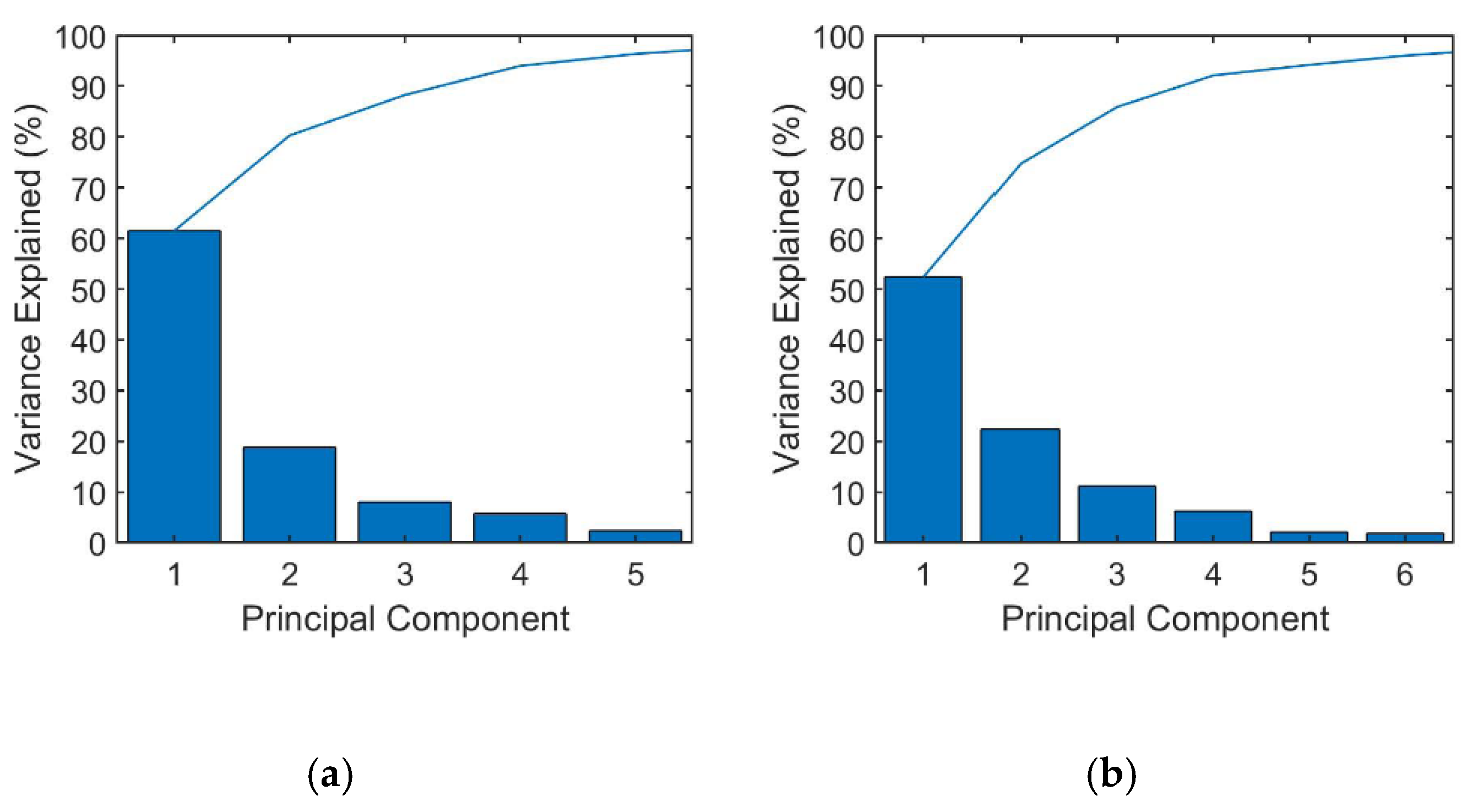
In this study, the initial thermochemical data of two cases were 50-dimensional data (including temperature and mass fractions of 49 species). We used MATLAB to perform PCA analysis of the data. Figure 1 shows can see that for both cases, the first five PCs contained more than 95% of the information of 50 scalars. In order to reduce computational cost, these five-PC datasets retained after rotated PCA were used for subsequent analysis.

3.2. Clustering Analysis

The application of techniques of artificial intelligence, which can be used for analysis of complex multivariate data and prediction of nonlinearities, can potentially be useful in analyzing data, including turbulent combustion. After using rotated PCA to extract useful data from the original by removing redundant information, it was necessary to analyze the data to distinguish the characteristics of different combustion states. One of the vital means in dealing with the data was to classify or group them into a set of categories or clusters. Clustering algorithm is a branch of machine learning and belongs to unsupervised learning. The goal of clustering is to separate a finite unlabeled data set into a finite and discrete set of natural hidden data structures. 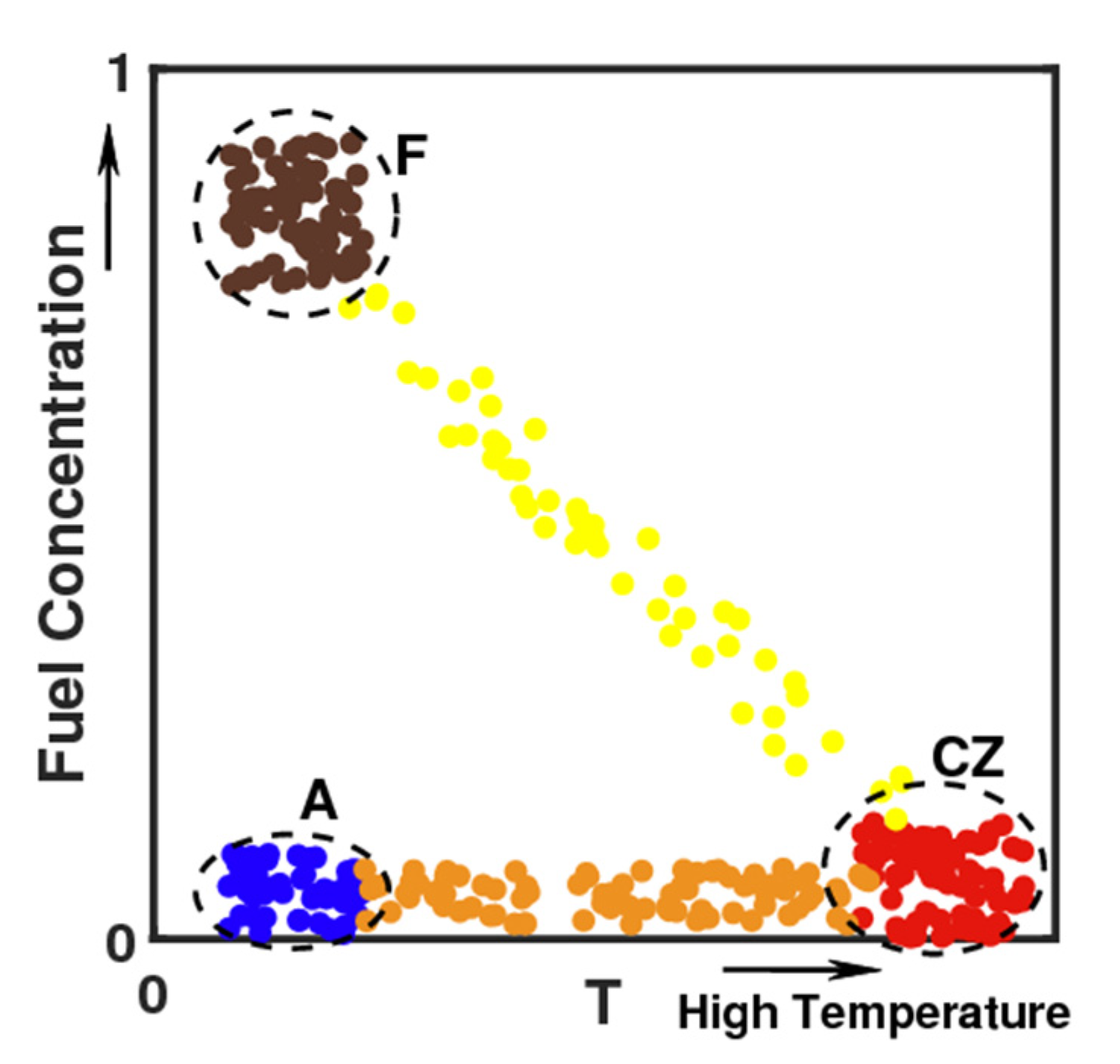Figure 2 shows a schematic diagram of combustion clustering, and scatters of temperature and fuel concentration are presented as an example. Clustering classification of scatters of low temperature and high fuel concentration represented fuel inlet; scatters of high temperature and low fuel concentration were located in the combustion zone; and the air inlet was characterized by low fuel concentration and low temperature. Connecting the fuel inlet and the combustion zone represented all reaction paths, while connecting the combustion zone and the air inlet was dominated by the heat transfer process. This diagram is only a two-dimensional diagram using fuel and temperature. If different scalars were used for analysis, the distribution of scatters would show different characteristics. For example, in the preheating area (yellow scatters in Figure 2) connecting the fuel inlet and the combustion zone, the concentration of CH₂O is very high, while it is very low in other regions. The concentrations of major products, such as H₂O, CO, and CO₂, were high in the region represented by orange in Figure 2. Although the high-dimensional scalar distribution was difficult to represent by a two-dimensional scatter diagram, the example in Figure 2 presents the multi-dimensional clustering analysis and can objectively classify multidimensional thermochemical data to distinguish various regimes.

The study can use many clustering algorithms, but here we adopted two of the more commonly used algorithms. K-means [24] clustering algorithm is the earliest proposed clustering algorithm, and the K-means and its variants have been widely studied and applied in different scientific fields. The K-means requires the user to pre-specify the number of clusters present in the dataset. The K-means algorithm partitions a given set of data in a manner such that the squared-error function is minimized for a pre-specified number of clusters. The squared error function ($E$) is defined as:

$$E={{\displaystyle \sum }}_{\mathrm{K}=1}^{\mathrm{K}}{{\displaystyle \sum }}_{\mathrm{x}ϵ{\mathrm{S}}_{\mathrm{k}}}\Vert \mathrm{X}-{\mathrm{Z}}_{\mathrm{k}}{\Vert }^2,$$

(1)

where K is number of specified clusters, the d-dimensional ${\mathrm{Z}}_{\mathrm{k}}$ denotes the center of kth cluster and Χ represents a d-dimensional data vector belonging to the cluster S_k. The K-means algorithm aims to minimize the sum of squared distances between all points and the cluster centers. Compared with other clustering algorithms, the K-means clustering has an obvious advantage of fast calculation speed [25], which is also the first clustering algorithm used in this study.

Furthermore, this study also adopted the self-organizing maps (SOM) neural network method [26] for data analysis to compare with the results using K-means to see the reliability of clustering. The SOM is an unsupervised learning method to analyze various data sets, including those with missing values, and Chen et al. [27] have demonstrated that the SOM is a superior clustering technique. The SOM performs dimensionality reduction and classification and projects a high-dimensional input space onto a low dimensional topology so as to allow the number of data clusters to be visualized/determined by manual inspection. The computational steps of SOM algorithm are described below.

Step 1 (Initialization): Let Xi, i = 1,2, …, n, be the d-dimensional vectors to be clustered. Select small random values for the initial weights, Wij(0), and fix the initial learning rate (${\hat{\mathsf{\alpha }}}_0$) and the neighborhood. Wij(0) is the d-dimensional weight vector associated with the node at location (i, j) of a 2-dimensional grid array

Step 2 (Determining the best matching unit (BMU)): Select a sample pattern, X, from the data set and determine the BMU (Cij) at training iteration t, using the minimum Euclidean distance criterion.

$$\Vert X-{\mathrm{W}}_{{\mathrm{C}}_{\mathrm{ij}}}\Vert =\underset{\mathrm{ij}}{\min }\Vert \mathrm{X}-{\mathrm{W}}_{\mathrm{ij}}\Vert ; \mathrm{i}=1,2\dots \mathrm{L}; \mathrm{j}=1,2\dots \mathrm{L};$$

(2)

where ||.|| is the Euclidean norm and L denotes the number of rows (and also columns) in the square 2-D SOM grid.

Step 3 (Weight updating): Update all the weights according to the Korhonen learning rule;

Step 4: Increment the iteration index, t, by unity and decrease the magnitude of the learning rate, ${\hat{\mathsf{\alpha }}}_0$(t), accordingly; shrink, then neighborhood, NC_ij(t) of the BMU

Step 5: Repeat steps 2–4 until the change in the weight magnitudes is less than the specified threshold or the maximum number of iterations is reached.

In this study, the input layer of SOM neural network were related variables of combustion (temperature and mass fractions of species), and the output layer was a multi-dimensional spatial model (neuron). The more neurons, the more details are represented. The neuron nodes of the input variables and the output variables were trained to generate the neuron with the smallest n-dimensional distance until the clustering result was obtained. Both clustering analyses were performed using MATLAB.

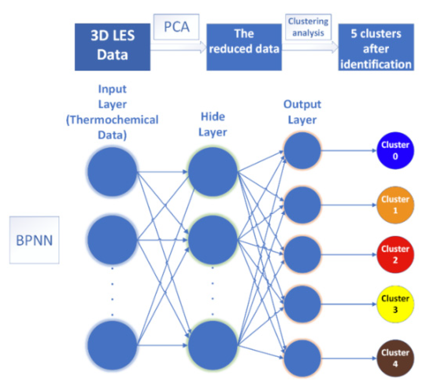
3.3. Back-Propagation Neural Network

Clustering analysis is a reliable classification method. However, if it is applied to a large amount of data, it still requires a great computational cost. Nonetheless, when performing local identification of the flow field, or when only limited data were available in the experiment, clustering analysis could be inaccurate. Previous study [4] has shown that supervised learning can offer accurate CRI after sufficient training. Artificial neural network (ANN) is a machine learning algorithm that simulates the human neural structure, which can be applied to both regression and classification problems. A standard neural network consists of many simple, connected processors called neurons, each producing a sequence of real-valued activations [28]. Back-propagation neural network (BPNN) algorithm is a simple and efficient method to correct the weight of neurons which was firstly developed by Dreyfus in 1973 [29]. The BPNN is a supervised learning algorithm. Its idea is to first calculate the gradient of the objective function to the output value of each neuron recursively through the chain rule, and then use the chain rule to calculate the gradient of the weight parameters on the edge. As shown is Figure 3, the network structure was a fully-connected neural network, which consisted of an input layer, an output layer, and a hidden layer.

The activation function adopted in this BPNN was the Softmax function to convert the output values of the multi-classification into relative probabilities:

$$\mathrm{Softmax}\left({\mathrm{y}}_{\mathrm{i}}\right)=\frac{{\mathrm{e}}^{{\mathrm{y}}_{\mathrm{i}}}}{{{\displaystyle \sum }}_{\mathrm{c}=1}^{\mathrm{C}}{\mathrm{e}}^{{\mathrm{y}}_{\mathrm{c}}}},$$

(3)

the y_i is the output value of the ith node, and C is the number of output nodes. Loss function is the cross-entropy loss function:

$$\mathrm{H}\left(\mathrm{y},{\mathrm{y}}^{*}\right)=-{\displaystyle \sum }\mathrm{y}·{\mathrm{lny}}^{*},$$

(4)

the y represents the exact probability distribution and y* represents the probability distribution of the predicted outcome.

In this study, the BPNN was trained by clustering results, and the network gradually “learns” the input/output relationship of interest by adjusting the weights to minimize the error between the actual and predicted output patterns of the training datasets. In specific, we used clustering analysis results of multiple instantaneous thermochemical data from the LESs of the HM1 and the Sandia Flame D as the training set, and then performed the BPNN predictions of two cases using the instantaneous thermochemical data at different times. The training of the BPNN was performed using the TensorFlow Python library. Once trained, returning the identification results from an input was almost instantaneous.

4. CRI with Clustering

The data of this study were the temperature and mass fractions of 49 species of the HM1 and the Sandia Flame D. Through rotated PCA, we retained five PCs as clustering input data. According to the analysis of the Davies-Bouldin index and flame structure, the optimal number of clusters was five, and

Table 1. Regimes represented by different clusters.

Number of Cluster	Regime
Cluster 1	Air (A)
Cluster 2	Co-flow (CO)
Cluster 3	Combustion Zone (CZ)
Cluster 4	Preheat (P)
Cluster 5	Fuel (F)

summarizes the five clusters representing five different states in the flames. Cluster 1 described environmental air. Cluster 2 represented the co-flow region, and cluster 3 referred to a state in which reactions were active, and the concentrations of active species, such as OH, were intense. Cluster 4 represented the combustion preheating stage, where temperature was not high, and the concentrations of some typical species, such as CH₂O, were intense, and cluster 5 represented the fuel inflow stream.

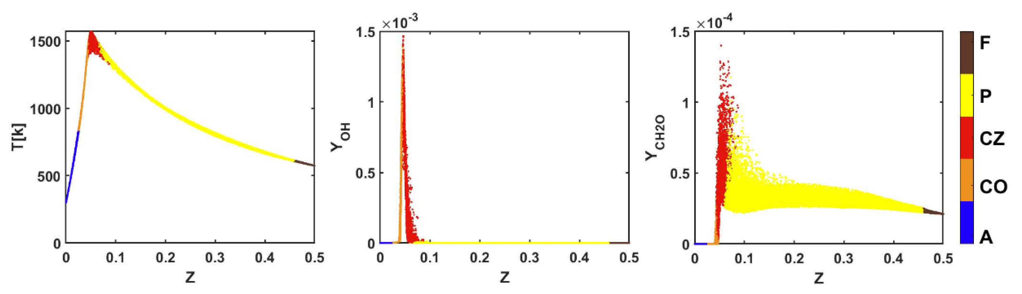
The analysis of artificial intelligence based on clustering algorithm is a mathematical technology capable of giving the quantitative characteristic indices of thermochemical data [30]. Figure 4 shows an example of scatter plots of temperature and mass fractions of OH and CH₂O in the mixture fraction space in the HM1, and reveals the differences between the five clusters and their physical characteristics. Z is element-based Bilger mixture fraction [25], which is defined as:

$$\mathrm{Z}=\frac{\frac{0.5\left({\mathrm{Y}}_{\mathrm{H}}-{\mathrm{Y}}_{\mathrm{H},2}\right)}{{\mathrm{W}}_{\mathrm{H}}}+\frac{2\left({\mathrm{Y}}_{\mathrm{O}}-{\mathrm{Y}}_{\mathrm{O},2}\right)}{{\mathrm{W}}_{\mathrm{C}}}-\frac{\left({\mathrm{Y}}_{\mathrm{O}}-{\mathrm{Y}}_{\mathrm{O},2}\right)}{{\mathrm{W}}_{\mathrm{O}}}}{\frac{0.5\left({\mathrm{Y}}_{\mathrm{H},1}-{\mathrm{Y}}_{\mathrm{H},2}\right)}{{\mathrm{W}}_{\mathrm{H}}}+\frac{2\left({\mathrm{Y}}_{\mathrm{O},1}-{\mathrm{Y}}_{\mathrm{O},2}\right)}{{\mathrm{W}}_{\mathrm{C}}}-\frac{\left({\mathrm{Y}}_{\mathrm{O},1}-{\mathrm{Y}}_{\mathrm{O},2}\right)}{{\mathrm{W}}_{\mathrm{O}}}},$$

(5)

where Yi is the total mass fraction of element i, and Wi is the atomic mass of element i. The subscripts 1 and 2 refer to values in the fuel and air streams. The calculations of Yi for elemental carbon, hydrogen, and oxygen should include all species in the mechanism. The characteristics of the environmental air regime included low temperature and low OH and CH₂O concentrations. In contrast, although the temperature and OH concentration in the fuel regime were also low, due to the chemical reactions gradually entering the preheating stage, it already had a certain concentration of CH₂O. The temperature in the co-flow regime was significantly higher than 800 K, but the concentrations of OH and CH₂O were low and close to the side of the environmental air. The characteristics of the combustion zone were significantly different than others. When the combustion was intense, the temperature was high. Owing to a large amount of OH production and CH₂O consumption, the OH concentration was high and close to the fuel regime, and the CH₂O concentration was high but close to the air regime. In the preheating stage of combustion, because there was not much OH production, although the temperature and CH₂O concentration were not low, the OH concentration was low.

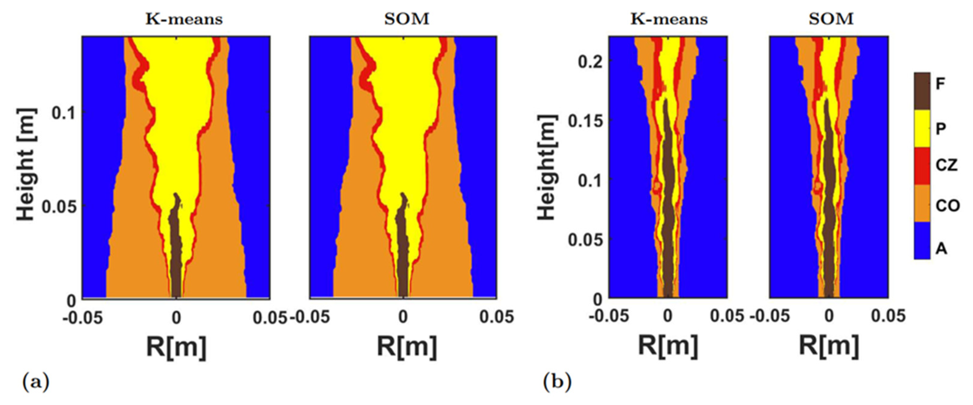
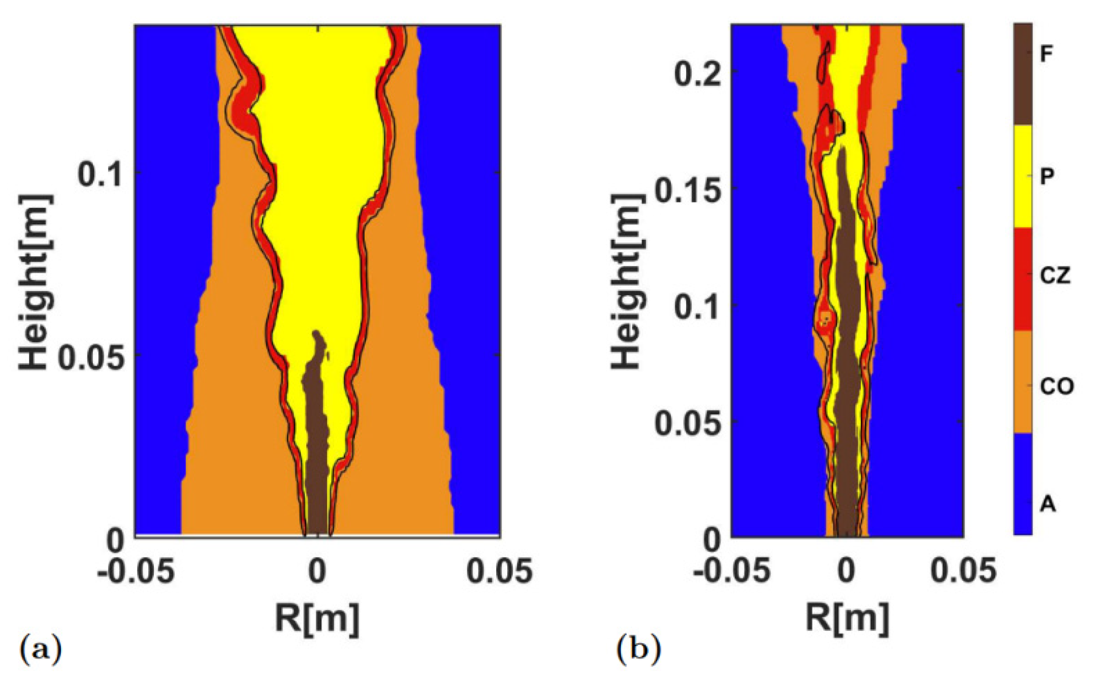
Figure 5 compares the clustering results obtained by two clustering algorithms (the K-means and the SOM) in the HM1 and the Sandia Flame D. R is the radial distance from the center. The correlation coefficients between the K-means and SOM results were 0.999 and 1.000 for the HM1 and the Sandia Flame D, respectively. This implied that the two clustering algorithms could deliver almost the same clustering results in the two flames, and the classifications embodied in the clustering would objectively represent the different quantitative characteristics in the flame data.

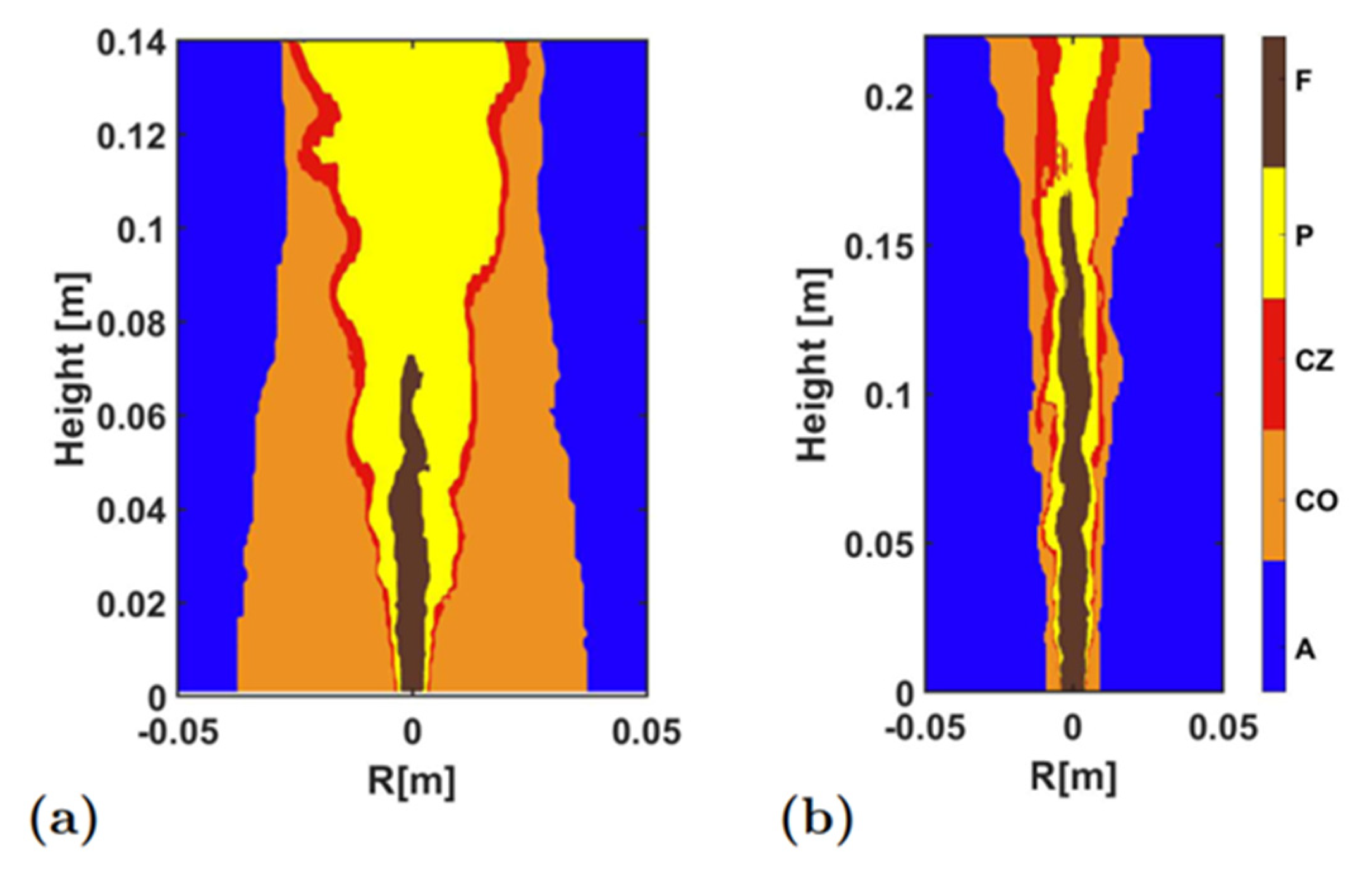
Furthermore, Figure 6 and Figure 7 compare the differences between the results obtained using the K-means clustering and the threshold method. Figure 6 embeds the isolines (20% of its maximum value) of HRR into the clustering results. It is a basic means to characterize the combustion zone with high HHR [3,8,9]. Since it is difficult to measure HRR directly in experiments, many methods [13] characterize flames by predicting HRR, and then measure the geometric parameters, such as flame thickness and wrinkle. It was evident that the combustion zone identified by the clustering algorithm was highly consistent with the results of the HRR threshold method. In addition, it should be noted that the clustering algorithm could not only judge the combustion zone, but also identify other characteristic regimes (such as the preheat zone), and the threshold method must use other variables, such as CH₂O, etc.

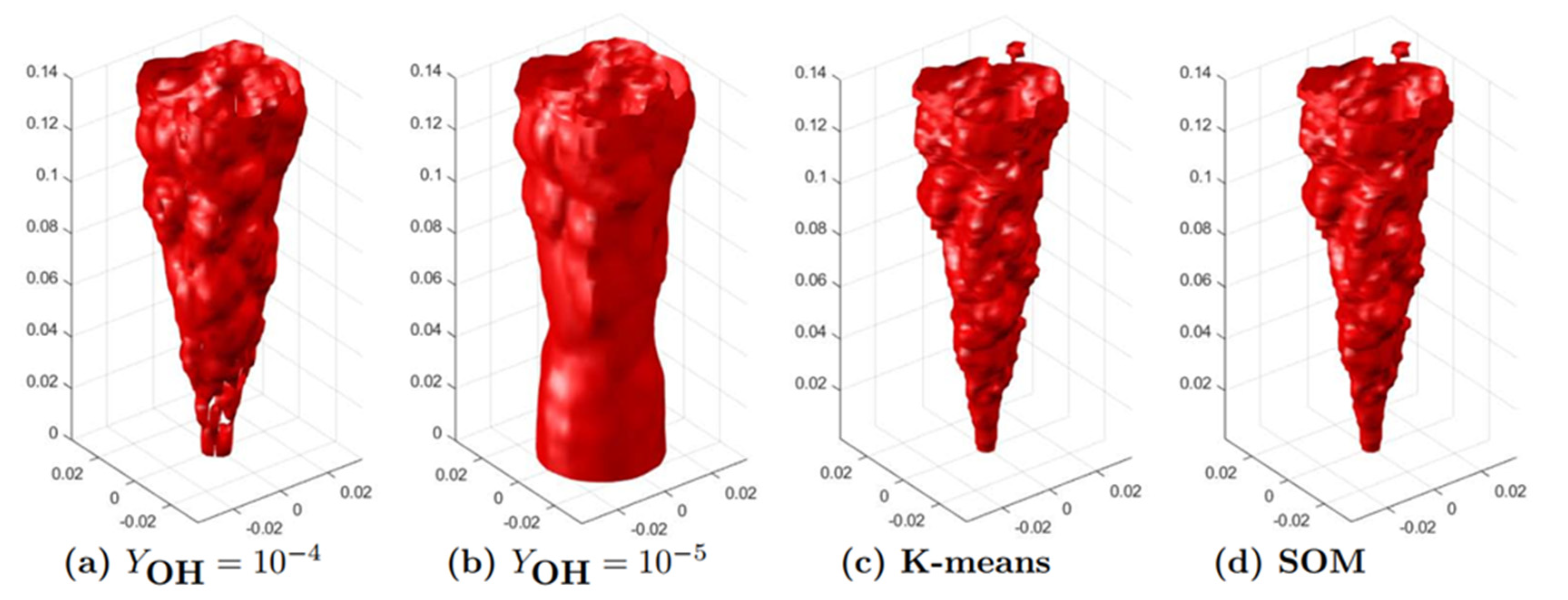
As mentioned earlier, the OH-threshold method is often used to represent the combustion zone [13]. However, the flame front would appear differently in shape and thickness when different critical values of OH concentration are used. As shown in Figure 7, the flame front structure in the HM1 case would be significantly different for using Y_OH = 10⁻⁴ and Y_OH = 10⁻⁵. For all threshold methods, including the GFRI method mentioned above, there exists the same problem of threshold selection. In specific, when using the threshold method to determine the combustion zone, if different variables are used, such as HRR or OH concentration, or the threshold value is different, these may affect the results, thus affecting further analysis, such as obtaining the flame lift-off height, flame thickness, etc. Using multidimensional clustering analysis algorithm to carry out CRI obviously would not produce such a problem. The frame front results detected using the K-means and the SOM are identical, indicating that the quantitative characteristic index given by unsupervised machine learning is more objective and reliable.

5. CRI with BPNN Trained by Clustering Results

Combustion regime identification with rotated PCA and clustering has been shown to be robust and accurate [30]. Although PCA can cut down the number of variables and reduce CPU cost for clustering, a large amount of computations is still required to process the data and predict the corresponding combustion regime. Moreover, in experimental measurements or industrial applications, it is usually difficult to obtain multiple scalar fields as the data source for clustering analysis, and clustering analysis with limited data could be fallacious. Therefore, this study attempted to adopt the supervised machine learning to provide an ultra-fast and reliable CRI based on limited thermochemical properties, and also tried to perform accurate CRI with fewer data, which is investigated in this section to the minimum data required for accurate CRI and the possible required data types.

For the evaluation of BPNN results, we still adopted the method of examining the flame structure, and compared it with the flame structure obtained using the cluster analysis. We also compared the BPNN result with the clustering result by three quantitative methods. Since the K-means CRI result and the SOM CRI result described above are nearly identical, we used the K-means result as the comparison object here. The accuracy rate, which is defined as the ratio of the number of correctly identified samples to the total number of samples, was used to evaluate the identification accuracy of the whole domain. The combustion zone is the focus of many studies. Thus, we can extract the data of combustion zone and binarize the flame into the flow field, and then calculate the correlation coefficient and the F₁ score between the two results. The F₁ score follows: 2/F₁ = (FP + TP)/TP + (FN + TP)/TP, where comparison results are divided into four categories, true positive (TP, where combustion zone identified using the K-means clustering is identified as combustion zone), false positive (FP, where non-combustion zone identified using the K-means clustering is identified as combustion zone), false negative (FN, where combustion zone identified using the K-means clustering is identified as non-combustion zone) and true negative (TN, where non-combustion zone identified using the K-means clustering is identified as non-combustion zone). Note that TN was not used in the evaluation of the F₁ score.

According to the corresponding scalars represented by the first few major PCs characterized by PCA shown in the previous study [30], and taking into account the chemical species that are usually measured in experiments, we used the five scalars, including temperature and mass fractions of CH₄, CO, OH, and CH₂O as the input data of the BPNN. Figure 8 shows the BPNN results of CRI using these five scalars. This was very consistent with the previous clustering results shown in Figure 4. In specific, the recognition accuracy in the HM1 was 98.64%, and the recognition accuracy in the Sandia Flame D was 98.88%. In both cases, selecting these five dimensions as the input data for the BPNN could accurately achieve CRI of the flame.

Considering the very limited data available for experimental measurements, in order to provide a simple method to determine the combustion regimes, we reduced the number of input variables step by step to see the accuracy of the BPNN results of CRI. It was also a test of the reliability of the BPNN method used in this CRI study and the minimum limit of input required for identification. Of course, reducing the dimension of the input data could also reduce the computational cost during CRI. 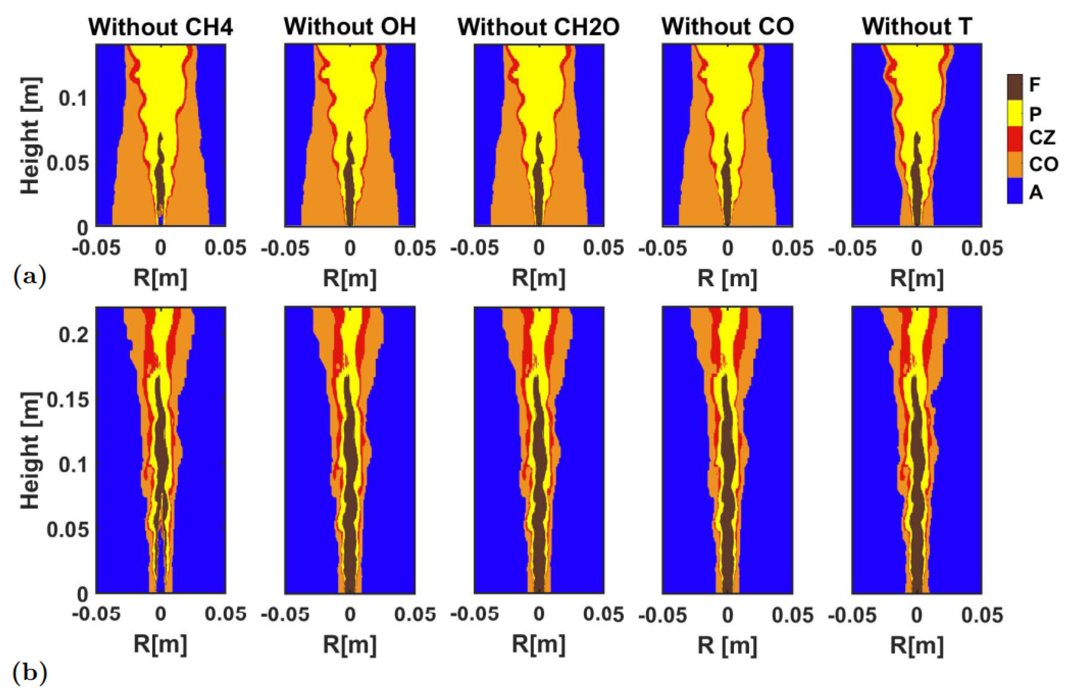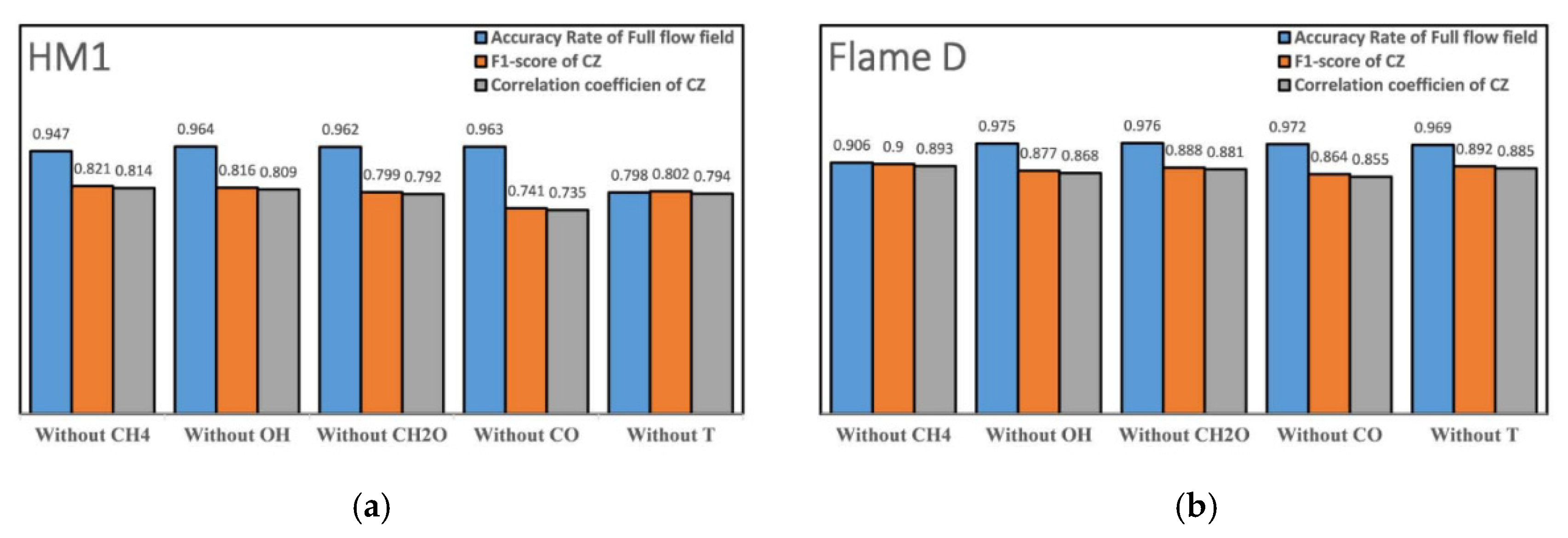Figure 9 shows the identification result after removing one of the five variables used in the identification shown in Figure 8, and Figure 10 presents quantitative indicators of identification accuracy. It was clear that, overall, the identification of four variables here were quite reliable. Overall, all identification accuracies were very high, remaining at a level of more than 95%. Except in the HM1, the identification accuracy dropped to almost 80% if the temperature was absent among the variables, due to the existence of large high-temperature co-flow region. In the Sandia Flame D, however, the pilot/co-flow region was small, so the absence of temperature did not affect the identification very much. In the Sandia Flame D, the most influential factor was the absence of fuel (i.e., CH₄). Since the identified fuel region was large, the absence of fuel reduced the identification accuracy to 90%. As for the identification of the combustion zone, all identifications maintained a high accuracy. The F₁ score and the correlation coefficient were maintained above 70%, and most of them were above 80%.

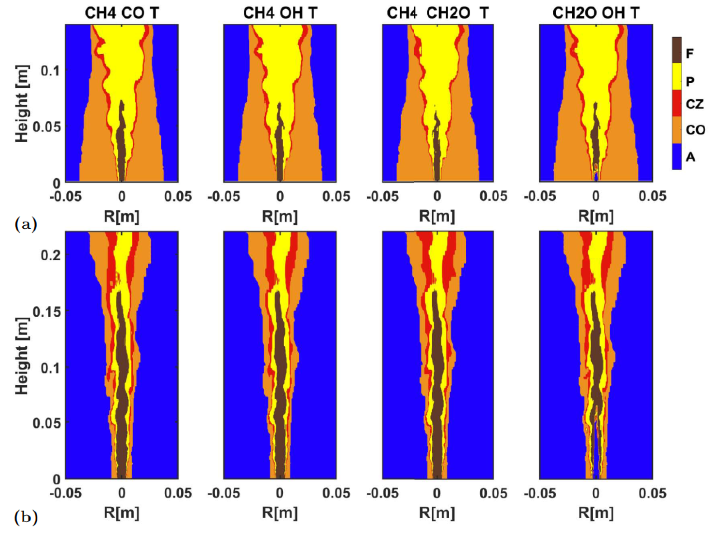
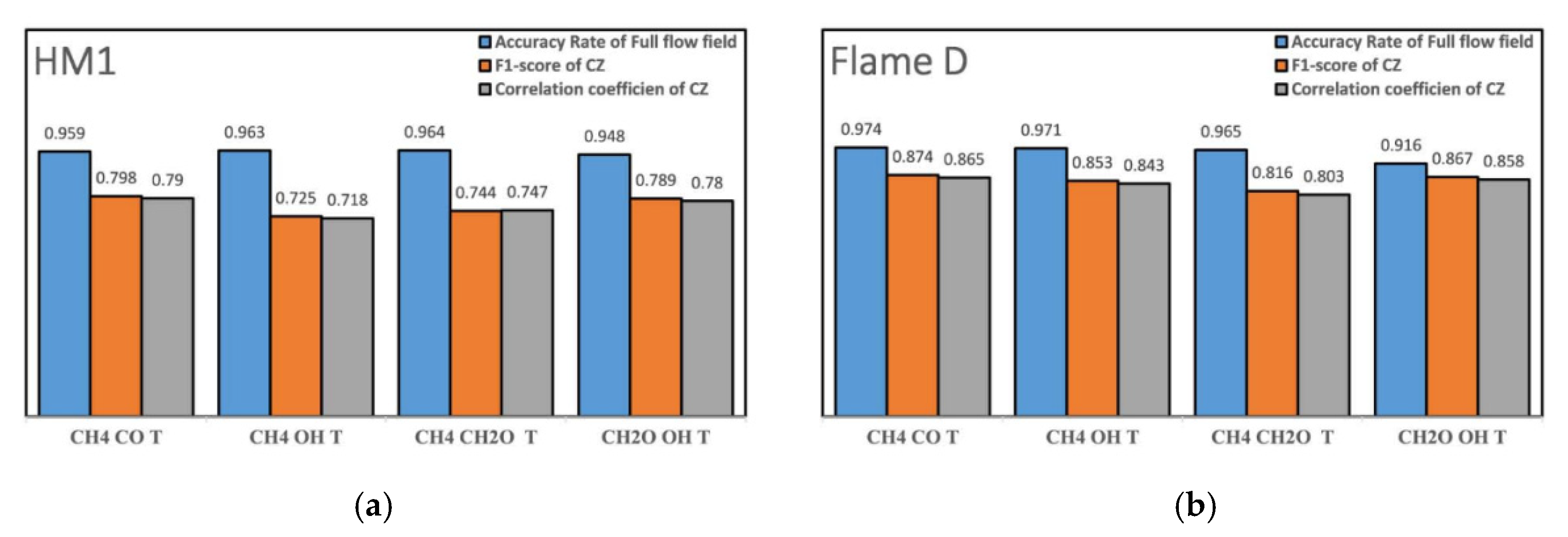
Furthermore, Figure 11 shows the identification result using three variables, and Figure 12 presents quantitative indicators of identification accuracy. Note that the identification accuracy in the HM1 was reduced to 85% without temperature, and, thus, the results without temperature input are not shown here. Again, the overall identification was still good. Obviously, the 3-dimensional CRI results in the presence of temperature were basically above 95%; except in the Sandia Flame D, where the absence of fuel made the identification accuracy lower, which was 91.6%. For the identification of the combustion zone, the F₁ value and the correlation coefficient were both higher than 0.7 for all tests. Especially the combinations of CH₂O-OH-T and CH₄-CO-T could better capture the combustion zone.

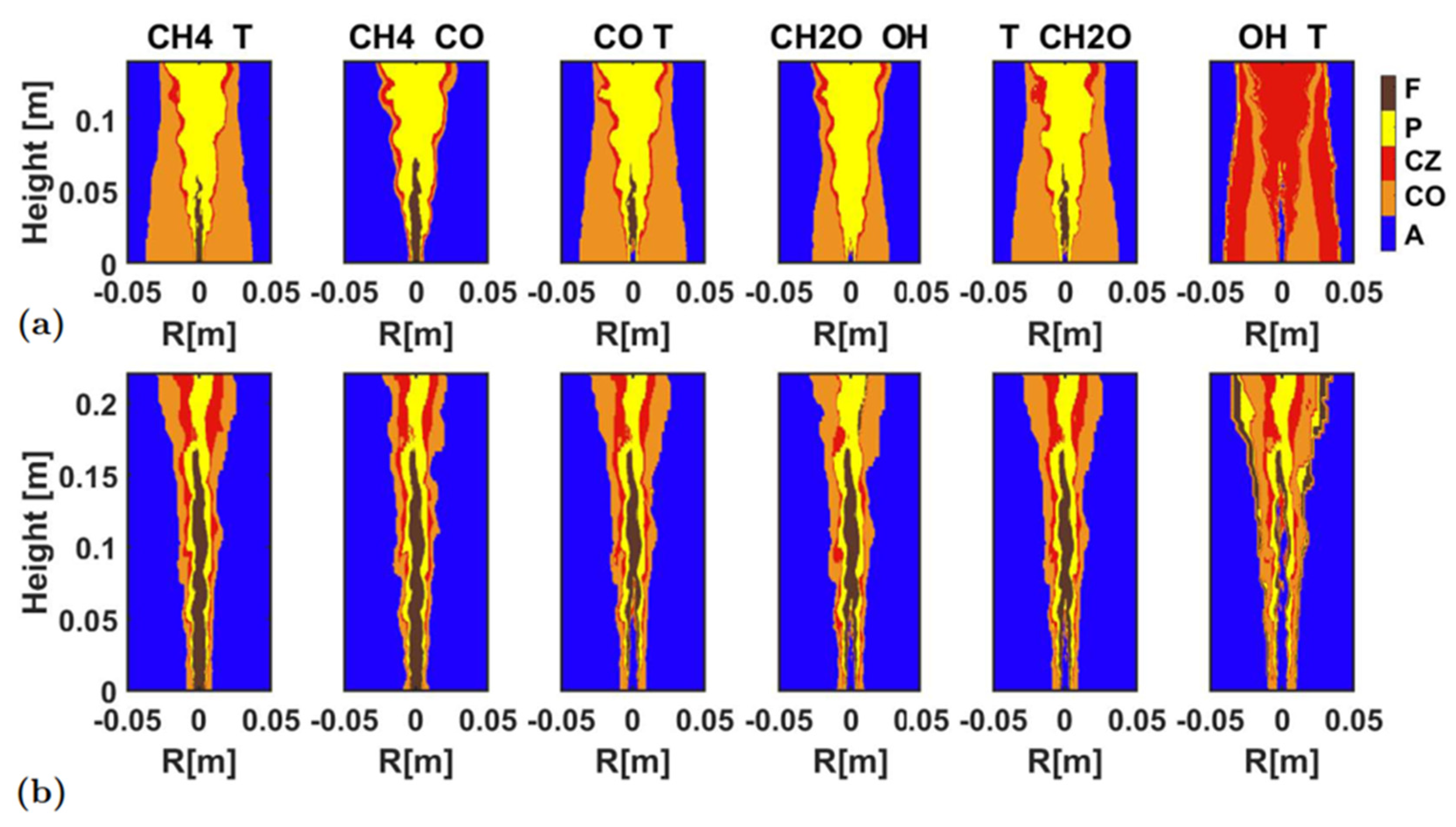
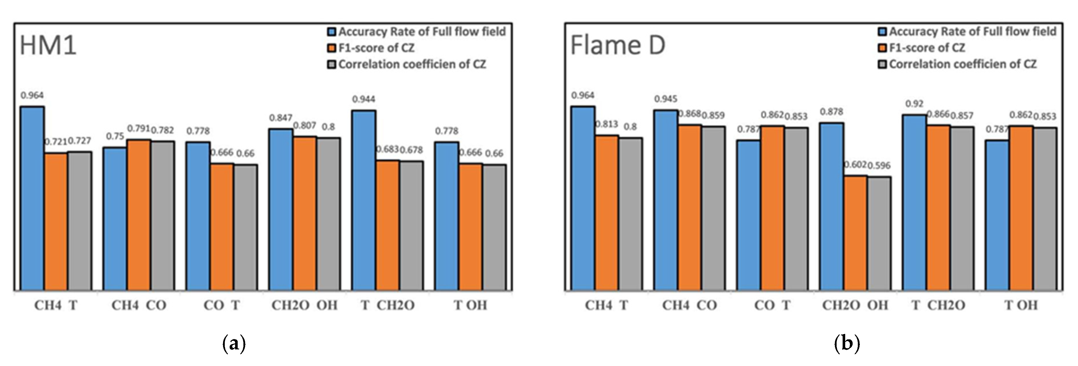
At last, Figure 13 shows the identification result using two variables, and Figure 14 presents quantitative indicators of identification accuracy. The overall identification was acceptable, except for the identification based on temperature and OH profiles. In the HM1, the combinations of CH₄-T and CH₂O-T yielded good overall identification accuracy, while for the combustion zone, the combinations of CH₄-CO and CH₂O-OH yielded better accuracy. In the Sandia Flame D, the combinations of CH₄-T, CH₄-CO and CH₂O-T yielded good overall identification accuracy, while for the combustion zone, the combinations of CH₄-CO and CH₂O-T yielded better accuracy. Overall, the CH₄-T combination yielded the best identification accuracy, both for the entire flame and the combustion zone. These two thermochemical quantities were also a group of scalars that could be relatively easily measured in real time in experiments.

6. Conclusions

A BPNN was trained to identify combustion regimes in two well-known turbulent non-premixed flames. The LES data was first processed with rotated PCA, and clustering analysis to generate a pixel-wise CRI database.

The application of rotated PCA can reduce 50-dimensional thermochemical data (including temperature and mass fractions of 49 species) to 5-dimensional input data, while retaining almost 95% of the information. This enables subsequent analysis to greatly reduce computation cost. Furthermore, the clustering analyses showed that these 5-dimensional data can be divided into 5 clusters, and, according to the thermochemical characteristics they represent, they are distinguished as: environmental air region, co-flow region, combustion zone, preheat zone and fuel stream. The results showed that these five regimes were well detected by the machine learning method with an accuracy of more than 98% using 5 scalars as input dataset.

Compared to other CRI approaches, such as the flame index method, the GFRI method etc., the proposed method avoids using any artificially determined thresholds for identification and does not require any scalar gradients. The computational cost of the method is very small. However, the CRI accuracy is quite satisfactory, for instance, even using the combined data of CH₄-T. The BPNN identification can achieve an accuracy of more than 95% for the entire flame. The method is a practical method to identify the combustion regime for industrial applications, and a support for further analysis of the characteristics in turbulent flames.