Numerical Simulation on Hydraulic Fracture Height Growth across Layered Elastic–Plastic Shale Oil Reservoirs

Abstract

Shale oil reservoirs are characterized by having various types of vertical sublayers, a large contrast in rock mechanical properties, well-developed bedding, and high clay content, which are likely to cause rock elastic–plastic deformation. In numerical simulations of hydraulic fracture (HF) propagation in the shale oil reservoirs, the effects of rock elastic–plastic deformation and complex bedding structure on the layer-crossing behavior of HF are not considered. To understand the mechanism of HF height growth in shale oil reservoirs, we used the cohesive zone method to establish an elastic–plastic finite element model of HF propagation by considering the effects of shell limestone interlayers, the Mohr–Coulomb yield criterion for shear–plastic failure, the cross-mechanical interaction between bedding and shale oil reservoir, and the complex situations such as the HF height across high-electrical resistivity bedding and high-conductivity fractures. The effects of internal friction angle, cohesion, layer stress contrast, fracture toughness, bedding bond strength, injection rate, elastic modulus, and bedding shear strength on HF height growth in shale oil reservoirs are studied, and the characteristics of HF width profile, injection pressure, failure mode, and maximum HF width are compared. Compared with the layer stress contrast, cohesion, internal friction angle, and fracture toughness, the injection rate, elastic modulus, and bedding shear strength and bond strength have a larger effect on the vertical HF width. Increment of the injection rate, decrease of the elastic modulus, and increment of the bedding shear strength and bond strength are favorable for HF height growth in the shale oil reservoir. As rock cohesion and internal friction angle increase, the HF width decreases. At the initial stage of fracturing fluid injection, the maximum HF height and injection pressure fluctuate. Lower cohesion and internal friction angle promote rock shear failure in HF height growth. Our study provides guidance for the stimulation of fracture crossing layers in the shale oil reservoirs.

1. Introduction

China has shale oil resources of about 27 × 10⁹ tons [1]. The Jiyang Depression is located in the southeast part of the Bohai Bay Basin, and the predicted shale oil reservoir resource there reaches 40.45 × 10⁸ tons. The commercial hydrocarbon flow has been obtained in over 40 wells, showing promising prospects [2]. The continental shale is generally in the middle diagenetic stage, and the shale is characterized by rapid variation in lithology, high clay content, and strong rock plasticity, which cause high breakdown pressure, a short HF propagation path, low fracturing fluid recovery, and low stable production. It is very difficult to form a complex fracture network in shale oil reservoirs [3,4,5,6].

The technology of fracture crossing layers is an effective stimulation method in the interbed reservoirs. There is a great difficulty in HF height growth in shale oil reservoirs due to significant stress contrast and strong rock plastic deformation. Compared with the conventional fracturing technology, the technology of high-viscosity fracturing fluid (≥60 mPa·s) and large injection rate (≥12 m³/min) increases the HF height by 40–58% and promotes HF height growth [3]. The stimulation technology of fracture crossing layers is feasible in shale oil reservoirs.

Many efforts have been focused on the study of HF height growth in the stimulation of layered shale oil reservoirs. HF vertical growth in the layered shale oil reservoir is controlled by reservoir properties such as horizontal stress difference, bedding strength, and bedding thickness, and treatment parameters such as fracturing fluid injection rate and viscosity [7,8,9,10,11,12].

HF propagates as a cross shape in the tight sandstone, as a straight shape in the sandstone developed with natural fractures (NFs), and as a stepped shape in the shale with developed bedding. The shale bedding restricted HF height growth [13,14]. Rock mechanical parameters, stage spacing, and fracturing stimulation technology are factors that affect fracture interaction in HF height growth in the horizontal well [15]. Li et al. [16] carried out numerical simulation of HF height growth in the coal bed and suggested that the in situ stress and interface strength of coal rock affect the behavior of HF propagation in the rock bedding. The larger vertical stress contrast coefficient and interface shear strength are favorable for HF height growth. The difference in elastic modulus and tensile strength between the coal bed and overlying strata is favorable for fracture height growth. The injection rate and spacing between the injection point and bedding should be optimized to promote HF propagation across the coal beds. Based on the true triaxial hydraulic fracturing physical simulation system, Hou et al. [17] studied HF propagation in the directional well in the sandstone and shale interbed reservoirs and suggested that wellbore azimuth and horizontal stress difference have a significant effect on HF propagation. The larger azimuth and the smaller horizontal stress difference cause more fracture distortion near the wellbore and are not conducive to vertical HF propagation or proppant migration within the fracture. The mudstone hinders vertical HF propagation. The higher stress contrast between sandstone and mudstone layers causes a larger hindering effect, and the HF is less likely to propagate to the mudstone layer from the sandstone layer.

The 2D, quasi-3D, and full 3D mathematical models for fracture crossing layers were established [18,19,20,21,22]. Perkins-Kern-Nordgren (PKN) and Kristianovich-Geertsma-de Klerk (KGD) models only consider HF height growth and cannot reflect the fracture length propagation behavior [23,24,25,26]. The quasi-3D or full 3D model considers HF height growth and 1D fluid flow along the fracture length; vertical fluid flow is neglected [27]. When the ratio of fracture length to HF height is greater than four, the quasi-3D failure model reflects the actual conditions. In fracturing of the low-permeability and thin interbed reservoirs, the HF height grows, and the ratio of fracture length to HF height is less than four. Then, 2D fluid flow occurs both along the fracture length and fracture height direction, and this is not consistent with the assumption that vertical fluid flow is neglected. Therefore, the quasi-3D model is not applicable [18,28]. Accordingly, a two-dimensional flow quasi-3D HF propagation model was proposed based on 2D flow in the low-permeability thin-interbed sandstone reservoirs. The model considers lateral and vertical fluid flow within the fracture. The full 3D simulation on fracture can reflect the behavior of HF propagation during HF crossing vertical layers. Lateral and vertical fluid flow and the upward and downward fracture extension to the caprock and bottom layer were calculated. Liu et al. [29] established a 3D finite element numerical model of HF height growth in the thick-layered reservoir based on hydro-mechanical coupling and rock mechanics and analyzed the effects of mudstone interlayer thickness, number, and perforation location on vertical HF propagation. Wang et al. [13] established a quasi-3D HF propagation numerical model for layered shale oil reservoirs by considering the interface strength, perforated position, and injection rate of fracturing fluid and applying the global embedded cohesive element. They also studied the behavior of HF propagation through multiple layers. Simulation of HF growth across layered shale oil reservoirs involves hydro-mechanical coupling, nonlinear failure, and transient problems and requires a large amount of computation and an efficient algorithm. The boundary element, extended finite element, discrete element, phase field, and numerical manifold methods have been applied in numerical simulation on hydraulic fracturing. Wang et al. [30] applied the proper generalized decomposition algorithm to the numerical simulation of hydraulic fracturing based on the idea of dimension reduction of stiffness matrix, and the algorithm is operated in the time domain and the spatial domain. The problems in the multiple dimensions are decomposed into those in the low-dimensional problems, and the real-time and fast solution of HF propagation is realized. However, the basis function needs to be decomposed and obtained in real time, and the programming process is troublesome.

The shale oil reservoir is characterized by lithology superposition and the development of natural structural planes such as sandstone argillaceous laminae and shale bedding. The criteria for interaction between HFs and natural structural planes are the key to the HF vertical propagation behavior [13,31,32]. The process of fracture crossing the bedding in the shale oil reservoir is a problem of hydro-mechanical coupling and rock failure. The effects of rock elastic–plastic deformation and bedding structure on HF height are not considered, and the mechanism of HF height growth is still not clearly defined.

We employed the cohesive zone-based finite element model to carry out numerical simulation on the vertical HF propagation behavior in fracture crossing layers in shale oil reservoirs by considering the elastic–plastic deformation and failure, and analyzed the effects of layer stress contrast, number, interlayer and reservoir thickness, bedding bond strength and inclination, fracturing fluid viscosity, and injection rate on HF initiation and propagation. Then, we determined the criterion for fracture across the bedding and the major factors for HF height growth.

The paper is organized as follows. The Methods and Theory section presents the governing equations, boundary conditions of fracture across layers, constitutive criteria for elastic–plastic deformation and failure, criteria for bedding and HF interaction, and validation examples. The Numerical Model section introduces the finite element model of fracture across layers, the physical parameters, and the stress profile. The Result section discusses the effects of internal friction angle, cohesion, layered stress contrast, fracture toughness, bedding bond strength, injection rate, elastic modulus, and bedding shear strength on the HF height growth in the shale oil reservoir through lamination, as well as differences in the HF width profile, injection pressure, tensile-shear failure mode, and the maximum HF width. The main conclusions of this study are summarized in the last section.

2. Methods and Theory

2.1. Equation of Mechanical Equilibrium

According to the classical elastic theory, the stress balance equation and boundary conditions are expressed as [30,31,32,33,34,35,36]:

$$\nabla \cdot \sigma =0\mathrm{in}\mathsf{\Omega }$$

(1)

$$\sigma \cdot n_t={\sigma }_H\mathrm{on}{\Gamma }_{\mathrm{L}}\cup {\Gamma }_{\mathrm{R}}$$

(2)

$$\sigma \cdot n_t={\sigma }_h\mathrm{on}{\Gamma }_{\mathrm{T}}\cup {\Gamma }_{\mathrm{B}}$$

(3)

$$\sigma \cdot n_f=p(s,t)\mathrm{on}{\Gamma }_f$$

(4)

$$u=0\mathrm{at}\mathrm{four}\mathrm{vortexes}\mathrm{in}\mathrm{the}\mathrm{rectangle}\mathrm{domain}\left(\mathrm{Figure}1\right)$$

(5)

where σ is the second-order Cauchy stress tensor acting on the entire rectangle in Figure 1; ε is the second-order strain tensor, u is the local displacement vector; p(s, t) is the fluid pressure on the fracture surface Γ_f; σ_H, and σ_h are the maximum and minimum horizontal principal stresses in the far-field; and n_t and n_f are the unit normal vectors at the outer boundary and the fracture boundary, respectively. ${\Gamma }_{out}={\Gamma }_L\cup {\Gamma }_R\cup {\Gamma }_T\cup {\Gamma }_B$ at the outer boundary and Γ_f at the inner boundary. Ω denotes the rectangle domain in Figure 1.

The constitutive equation between the stress tensor and the strain tensor is expressed as:

$${\sigma }_e=D:\epsilon$$

(6)

$$\epsilon ={\nabla }^{s}u=\frac{1}{2}\left(\nabla u+\nabla u^{\mathrm{T}}\right)$$

(7)

where D is the elastic coefficient matrix. For anisotropic rock under plane strain states, we have:

$$D=\frac{E}{1-{\nu }^2}\left[\begin{array}{ccc}1& \nu & 0\\ \nu & 1& 0\\ 0& 0& \frac{1-\nu }{2}\end{array}\right]$$

(8)

where E is the rock elastic modulus, ν is Poisson’s ratio, ${\nabla }^s$ is the symmetric operation symbol of the tensor, and ${\sigma }_e$ is the Biot effective elastic tensor.

According to the definition of effective stress, the Cauchy stress is decomposed as follows:

$${\sigma }_e=\sigma -\alpha p_{p}I$$

(9)

where p_p is the pore pressure acting on the rock matrix; α is the Biot elastic coefficient, α ∈ [0,1]; and I is the unit tensor. The value of α depends on the magnitude of the increment of pore pressure in the fracture and the decrease of total stress around the rock [37,38,39,40]. If the former is higher than the latter, α = 0.95; otherwise, α = 1 [37,38].

2.2. Equation of Flow Pressure in Hydraulic Fracture

We assumed that (i) there was no supply of fluids from the fracture walls and (ii) there was a source of fluid with flow rate Q₀ as the injection point inside the fracture. According to the lubrication equation in fluid mechanics, the continuity equation of Poiseuille planar flow between two parallel plates is expressed as:

$$\frac{\partial w}{\partial t}=\frac{\partial }{\partial s}\left(\frac{w^3}{12\mu }\frac{\partial p}{\partial s}\right)+Q_0\mathrm{in}{\mathsf{\Omega }}_{\mathrm{f}}$$

(10)

$$k=\frac{w^3}{12\mu }$$

(11)

$$w=\left(u^{+}-u^{-}\right)\cdot n_f\left|{}_{{\Gamma }_f}\right.$$

(12)

$$\frac{w^3}{12\mu }\frac{\partial p}{\partial n}=0\mathrm{at}\mathrm{two}\mathrm{fracture}\mathrm{tips}$$

(13)

where w is the HF width; μ is the fracturing fluid viscosity; Q₀ is the source term (i.e., the injection rate of fracturing fluid within the wellbore); Ω_f is the fracture area; k is the fracture permeability calculated according to the cubic law in Equation (11); u⁺ and u⁻ are the displacement vector on fracture face; and s is the abscissa of the HF. Due to the cubic term of the fracture width, Equation (10) is a nonlinear transient equation.

2.3. Criterion for Fracture Crossing Bedding

When the HF encounters the bedding or weak interfaces in shale oil reservoirs, the HF crosses the bedding and is diverted, arrested, and dilated. The behavior of HFs and bedding interaction depends on in situ stress, the mechanical property of rocks and NFs, rheological property of fracturing fluid, and injection rate. A lot of efforts have been put into theoretical and experimental study on interaction between HFs and NFs, and the criterion for fracture interaction is proposed.

As shown in Figure 2, the intersection angle between the HF and the bedding planes is β. According to Renshaw and Pollard’s intersection criterion, the bedding plane is regarded as a friction interface, and the no-slip conditions along the surface of bedding plane are expressed as [33,34,35,36,37,38,39,40]:

$$\left|{\tau }_{\beta }\right|<S_0-\lambda {\sigma }_{\beta y}$$

(14)

$${\tau }_{\beta }=K\sin \frac{\theta }{2}\sin \frac{3\theta }{2}\sin 2\beta +K\sin \frac{\theta }{2}\cos \frac{3\theta }{2}\cos 2\beta -\frac{{\sigma }_H-{\sigma }_h}{2}\sin 2\beta$$

(15)

$$\begin{array}{l}{\sigma }_{\beta y}=K+K\sin \frac{\theta }{2}\cos \frac{3\theta }{2}\cos 2\beta -K\sin \frac{\theta }{2}\cos \frac{3\theta }{2}\sin 2\beta +\frac{{\sigma }_H+{\sigma }_h}{2}\\ -\frac{{\sigma }_H-{\sigma }_h}{2}\cos 2\beta \end{array}$$

(16)

$${\cos }^2\frac{\theta }{2}{K}^2+2\left[\left(\frac{{\sigma }_H-{\sigma }_h}{2}\right)\sin \frac{\theta }{2}\sin \frac{3\theta }{2}-T\right]K+\left[T^2-{\left(\frac{{\sigma }_H-{\sigma }_h}{2}\right)}^2\right]=0$$

(17)

where λ is the friction coefficient of the NF surface; S₀ is the cohesion force of the NF surface; τ_β and σ_βy are the shear stress and normal stress on the NF surface, respectively; θ = β or β-π; β is the intersection angle between the NF and the HF; σ_H and σ_h are the maximum and minimum horizontal stress in the far-field, respectively; T = T₀ − [(σ_H-σ_h)/2]; T₀ is the rock tensile strength; K is the root of Equation (17) when σ₁ = T₀ and σ₁ is calculated in Equations (18)–(21); K_I is the I-type stress intensity factor at the fracture tip; r and α are the polar coordinates at the fracture tip; and σ_x, σ_y, and τ_xy are the stress components, expressed as follows:

$${\sigma }_1=\frac{{\sigma }_x+{\sigma }_y}{2}+\sqrt{{\left(\frac{{\sigma }_x+{\sigma }_y}{2}\right)}^2+{\tau }_{xy}^2}$$

(18)

$${\sigma }_x={\sigma }_H+\frac{K_I}{\sqrt{2\pi r}}\cos \frac{\alpha }{2}\left(1-\sin \frac{\alpha }{2}\sin \frac{3\alpha }{2}\right)$$

(19)

$${\sigma }_y={\sigma }_h+\frac{K_I}{\sqrt{2\pi r}}\cos \frac{\alpha }{2}\left(1+\sin \frac{\alpha }{2}\sin \frac{3\alpha }{2}\right)$$

(20)

$${\tau }_{xy}=\frac{K_I}{\sqrt{2\pi r}}\sin \frac{\alpha }{2}\cos \frac{\alpha }{2}\cos \frac{3\alpha }{2}$$

(21)

2.4. Constitutive Equation of Elastic and Plastic Deformation

In rock mechanics, the Mohr–Coulomb criterion is used to describe the shear failure behavior of rock and reflects the difference in compressive strength and tensile strength and the sensitivity to hydrostatic pressure. For the positive tensile stress, the Mohr–Coulomb criterion for shear failure in the form of principal stress is expressed as [34,35,36,37,38,39,40]:

$$F=\left({\sigma }_1-{\sigma }_3\right)+\left({\sigma }_1+{\sigma }_3\right)\sin \varphi -2c\cos \varphi =0$$

(22)

where σ₁ > σ₂ > σ₃ are the principal stress, and c and $\varphi$ are the cohesion force and the internal friction angle, respectively.

The Mohr–Coulomb criterion for tensile failure is expressed as:

$$-{\sigma }_3\ge f_t$$

(23)

In the π plane, the Mohr–Coulomb criterion for tensile failure is expressed as an equilateral triangle, which consists of three planes that are perpendicular to the principal stress axis in the yield surface in the principal stress field. The Mohr–Coulomb criterion for shear failure is a pyramid hexagon in the stress space, and the central axis coincides with the isocline.

The constitutive model of rock materials is usually expressed in the form of stress invariant as follows:

$${\sigma }_m=\frac{{\sigma }_1+{\sigma }_2+{\sigma }_3}{3}$$

(24)

$$\overline{\sigma }=\sqrt{\frac{1}{2}\left(s_x^2+s_y^2+s_z^2\right)+{\tau }_{xy}^2+{\tau }_{xz}^2+{\tau }_{yz}^2}=\sqrt{J_2}$$

(25)

$$J_3=s_x{s}_y{s}_z+2{\tau }_{xy}{\tau }_{xz}{\tau }_{yz}-s_x{\tau }_{yz}^2-s_y{\tau }_{xz}^2-s_z{\tau }_{xy}^2$$

(26)

where σ_m is the average stress, $\overline{\sigma }$ is the equivalent stress, and J₂ and J₃ are the second and third invariants of stress deviance, respectively: s_x = σ_x − σ_m; s_y = σ_y − σ_m; s_z = σ_z− σ_m.

Lode angle is expressed as:

$$\theta =\frac{1}{3}{\sin }^{-1}\left(-\frac{3\sqrt{3}}{2}\frac{J_3}{{\overline{\sigma }}^3}\right),\begin{array}{cc}& -{30}^{\circ }\end{array}\le \theta \le {30}^{\circ }$$

(27)

The principal stress in the form of the strain invariant is expressed as:

$$\left\{\begin{array}{c}{\sigma }_1=\frac{2}{\sqrt{3}}\overline{\sigma }\sin \left(\theta +{120}^{\circ }\right)+{\sigma }_m\\ {\sigma }_2=\frac{2}{\sqrt{3}}\overline{\sigma }\sin \left(\theta \right)+{\sigma }_m\\ {\sigma }_3=\frac{2}{\sqrt{3}}\overline{\sigma }\sin \left(\theta -{120}^{\circ }\right)+{\sigma }_m\end{array}\right.$$

(28)

Then, the Mohr–Coulomb criterion for shear failure in the form of stress invariant is expressed as:

$$F={\sigma }_m\sin \varphi -\overline{\sigma }K\left(\theta \right)-c\cos \varphi =0$$

(29)

where $K\left(\theta \right)=\cos \theta -\frac{1}{\sqrt{3}}\sin \varphi \sin \theta$.

The Mohr–Coulomb criterion for tensile failure in the form of stress invariant is expressed as [34]:

$$F=-\frac{2}{\sqrt{3}}\overline{\sigma }\sin \left(\theta -{120}^{\circ }\right)-{\sigma }_m-f_t=0$$

(30)

where f_t is the rock tensile strength.

2.5. Model Validation

To verify the reliability of the model of HF height growth in layered shale oil reservoirs, the finite element numerical solution is compared with the analytical solution of the KGD model, where the fracture length and width are expressed as [37,38]:

$$L_{frac}(t)=1.078{\left(\frac{E^{\prime }{q}_0^3}{{\mu }_f}\right)}^{1/6}{t}^{2/3}$$

(31)

$$w_0^h(t)=2.36\left(\frac{{\mu }_f{q}_0^3}{E^{\prime }}\right)t^{1/3}$$

(32)

where t is the injection time; q₀ is the injection rate; μ_f is the fracturing fluid viscosity; E′ is the plane–strain modulus, and E′ = 2G/(1 − ν); G is the shear modulus of shale oil reservoir, and ν is Poisson’s ratio.

To reduce the calculation amount, a 1/2 symmetric finite element model was applied. A finite element model with a length of 100 m and a width of 120 m was established and meshed with 21,280 plane–strain elements with pore pressure degree of freedom, and the rectangle elements integrated displacement field and pore pressure. The injection point was set at the midpoint of the left boundary. The injection rate per unit thickness was 2 L/s, the rock shear modulus was 8.3 GPa, Poisson’s ratio was 0.2, the fracturing fluid viscosity was 1 mPa·s, and the fluid bulk modulus was 2.2 GPa. A total of 133 cohesive elements with pore pressure degrees of freedom were embedded along the central axis, and the initial HF width was 0.002 mm. Figure 2 compares the finite element numerical solution and the analytical solution, which have a good agreement, and verifies that the model in this study is relatively reliable.

3. Finite Element Model of HF Height Growth

The case in this study is from a continental shale oil reservoir in China’s Fuxing block, where three wells drilled in Dongyuemiao Member are in Bashansi syncline, with a wide and gentle structure, no faults developed, reservoir porosity of 4.5–5.3%, inorganic pores developed, organic pores underdeveloped, mesopores and macropores dominating vertical limestone interlayers (>80%), and great layered stress contrast. The limestone shows the differentiated planar distribution. The shell limestone is characterized by high compressive strength (225–234 MPa), tensile strength, and fracture toughness. Clay mineral content is 48–62%, which results in strong water sensitivity. The mineral-based brittleness index is 28–32%. Young’s modulus is 13–26 GPa.

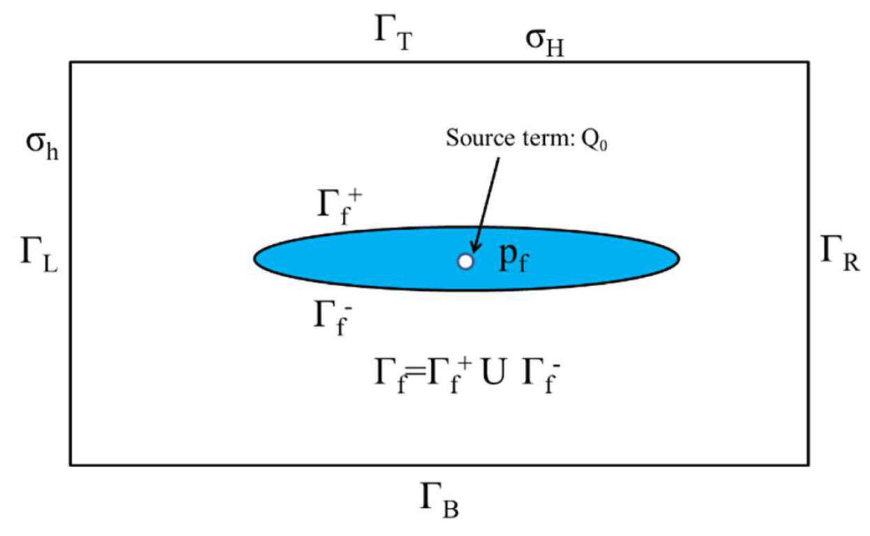
To reveal the HF height propagation growth and interaction between HFs and bedding in the fracturing of the shale oil reservoir, a 2D finite element model was established, with the injection point at the center (Figure 3). There are 5 sublayers with a total thickness of 25 m, including No.1 sublayer at the depth of 2865–2860 m and with σ_H and σ_h of 59 MPa and 56.8 MPa, respectively, No.2 sublayer at the depth of 2858–2855 m with σ_H and σ_h of 59 MPa and 57 MPa, respectively, No.2 shell layer at the depth of 2860–2858 m with σ_H and σ_h of 58 MPa and 55 MPa, respectively, No.3 sublayer at the depth of 2855–28,526 m with σ_H and σ_h of 60 MPa and 58 MPa, respectively, No.3 shell layer at the depth of 2853–2850 m with σ_H and σ_h of 62 MPa and 60 MPa, respectively, No. 4 sublayer at the depth of 2848–2845 m with σ_H and σ_h of 62 MPa and 60 MPa, respectively, No. 4 shell layer at the depth of 2850–2848 m with σ_H and σ_h of 60 MPa and 58 MPa, respectively, and No. 5 layer at the depth of 2845–2840 m with σ_H and σ_h of 55 MPa and 52 MPa, respectively.

The finite element model has a total of 47,299 nodes, and the rock matrix adopts 46,898 CPE4P plane strain elements with pore pressure degrees of freedom. A total of 500 COH2D4P elements were embedded in the direction of HF height growth (Figure 4). The cross-cohesive elements were programmed with the Python script. To create the continuous fluid pressure in HF height and bedding, a shared pore pressure node was set at the intersection. To eliminate the boundary effect in numerical simulation, a 50 m × 50 m hollow square was placed outside the 25 m × 25 m shale oil reservoir area. The hollow square area and the 25 m × 25 m shale oil reservoir area were connected with the “tie” keyword in the ABAQUS input file.

4. Results and Analysis

The input parameters in the numerical simulation are listed in

Table 1. Input parameters in numerical simulation on HF height growth in the shale oil reservoir.

Parameters	Units	Value
Porosity	Decimal	0.05
Initial pore pressure	MPa	49
Poisson’s ratio	Decimal	0.25
Elastic modulus	GPa	25
Cohesion	MPa	17.45
Internal friction angle	°	34.23
Permeability	mD	0.01
Rock tensile strength	MPa	3
Rock shear strength	MPa	10
Bedding tensile strength	MPa	6
Bedding shear strength	MPa	20
Rock fracture energy	Pa·m	600/600/2000
Bedding fracture energy	Pa·m	1200/1200/4000
Leakoff coefficient	m/(Pa·s)	1 × 10−14
Liquid viscosity	mPa·s	10
Injection rate	m3/min	12
Vertical stress	Vertical stress/MPa	71
Dilation angle	Dilation angle/°	0
Shell limestone elastic modulus	GPa	35
Shell limestone Poisson’s Ratio	Decimal	0.15

. The cohesion layer model was adopted. The criterion for damage and fracture initiation was the nominal quadratic stress criterion (QUADS). The damage evolution criterion was the energy-based BK fracture criterion [20]. The elastic–plastic deformation of shale oil reservoir during hydraulic fracturing was described with the Mohr–Coulomb criterion for tensile-shear failure, and analysis was completed in two steps. The first step is the Geostatic analysis of in situ stress balance and provides the initial stress field for hydraulic fracturing. The stress profile is shown in the Finite Element Model of HF height Growth section. The lateral stress is σ_h in each small layer, and the stress loaded vertically is the vertical stress 71 MPa in Table 1. The second step is the Soils hydro-mechanical coupling analysis and simulates HF propagation, the fluid pressure in the fractures, and the HF width, which are solved with the implicit finite element discretization method and the adaptive time step. The parameters in Table 1 are used as the base case, and the parameters are changed in different cases. A large number of nodes in this example, strong nonlinearity in hydro-mechanical coupling problems, and the interaction between HFs and bedding required a large amount of calculation. Numerical simulation was carried out in the high-performance Sugon computing cluster in Beijing Institute of Petrochemical Technology by parallel computing mode using 24 cores.

4.1. Effects of Bedding Shear Strength

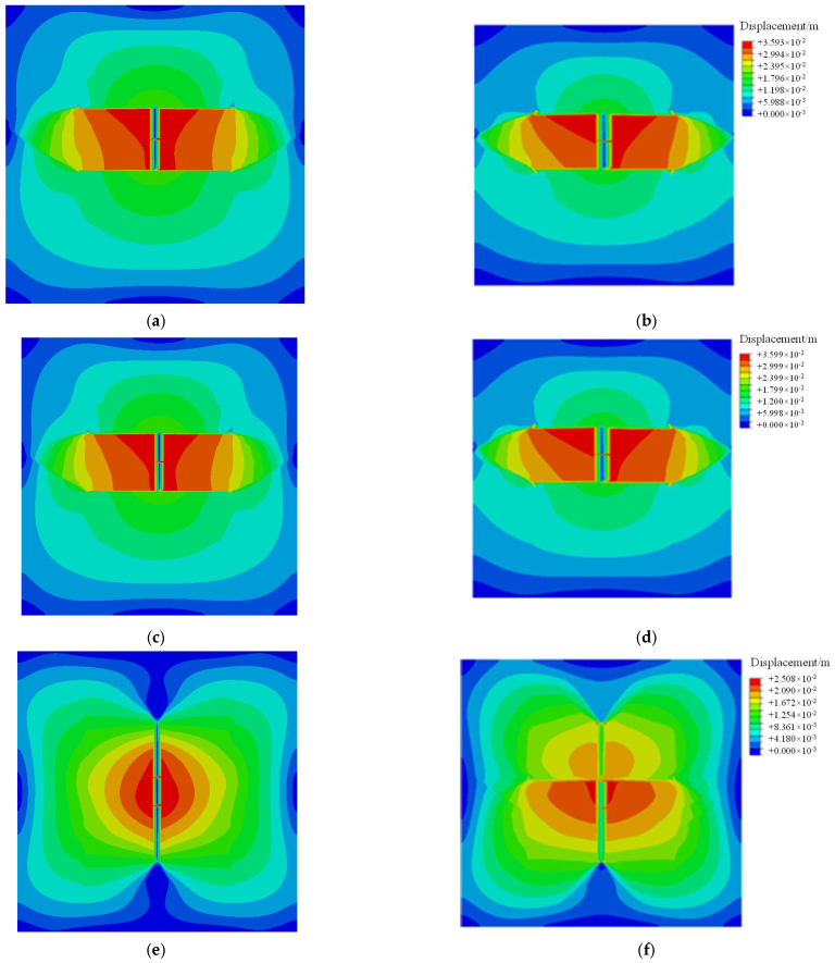
The core data show that the bedding is relatively developed in shale oil reservoirs, and the bedding’s mechanical strength affects HF height growth in the shale oil reservoir. Shear strength is a mechanical property of bedding. Laboratory experiments show that small displacement of shear slip occurs before the HF approaches the bedding. After the hydraulic fracture intersects with the bedding, shear failure and slippage occur in the bedding due to the effects of injected fluids. The shear-slippage displacement in this process is about 2–10 times that before fracture intersection. The maximum shear slip displacement and peak displacement rate of bedding increase as the deviatoric stress increases and the higher deviatoric stress enhance shear and slippage in NFs. Thus, these are the effects of bedding shear strengths (12 MPa/16 MPa/20 MPa) on the HF height growth in the layered shale oil reservoirs.

The displacement field under different bedding shear strengths is shown in Figure 5. Due to the non-uniform vertical stress profile, the displacement field above and below the injection point shows an asymmetric distribution. The above displacement is higher than the below displacement, indicating the larger fracture width above the injection point. When the shear strength of the bedding is high (20 MPa), the HF height grows vertically across the shale oil reservoir, and the HF height grows over a large distance across the bedding. When the shear strength of the bedding is low (12 MPa), the HF height is likely to be diverted to the bedding, and there is a large difficulty in vertical HF propagation. In Figure 5a–d, the HF height is diverted to the two beddings around the injection point. In base cases in Figure 5e,f, the fracture almost grows vertically and is only diverted to one bedding, and the bedding has little effect on the HF height growth. The higher shear strength of bedding enhances HF height growth across more reservoirs and communication with reservoirs.

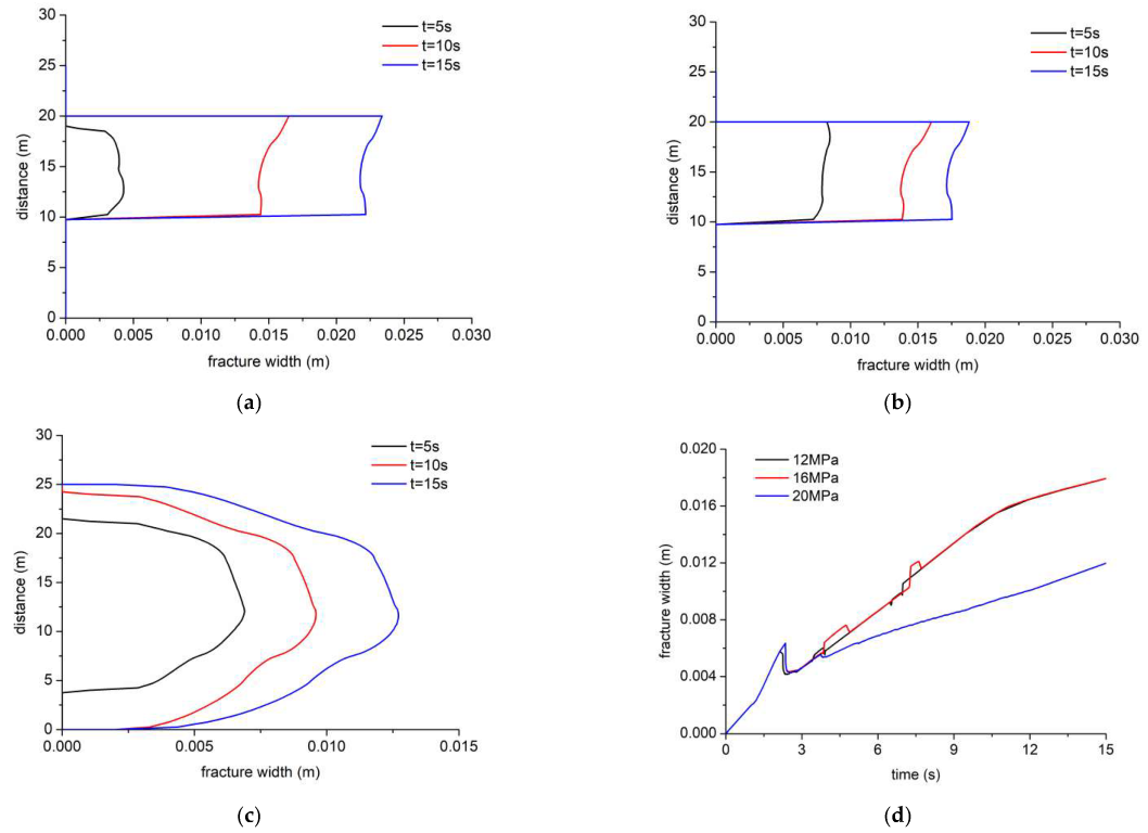
The HF width under different shear strengths is shown in Figure 6. In Figure 6a,b, the bedding shear strength is relatively low, and the vertical HF height is about 10 m. After 10 s of injection, the fracture interacts with the bedding vertically, and is diverted and propagates along with the bedding. The HF height does not grow. In Figure 6c, the bedding shear strength is relatively high, the vertical HF height is about 25 m after 15 s of injection. The fracture growth height increases by 1.5 times as the bedding shear strength increases by 8 Mpa, which is consistent with the results in Figure 5. The maximum HF width under different bedding shear strengths is shown in Figure 6d. The maximum HF width curves coincide when the bedding shear strengths of 12 Mpa and 16 Mpa. As the shear strength increases, the maximum HF width decreases, which is due to the fact that the fracture propagates vertically and the HF width decreases at the injection point.

The injection pressure and the ratio of tensile-shear failure under different shear strengths are shown in Figure 7. As the bedding shear strength increases, the number of injection pressure fluctuation reduces (Figure 7a). When the bedding shear strength is low, the injection pressure fluctuates significantly at the early stage, as the HF interacts with the bedding vertically, and a relatively complex fracture network is formed. The injection pressure has little difference under different shear strengths. After 9 s of injection, the injection pressure is slightly lower under the higher bedding shear strength, and vice versa. Due to interaction between bedding and HF height growth, opening of fractures requires high energy. When the bedding strength is high, the tensile failure ratio reaches about 80% (Figure 7b). When the fracture bedding is low, the tensile failure ratio is about 10%, the shear failure is dominant, and the bedding is opened by shear slippage.

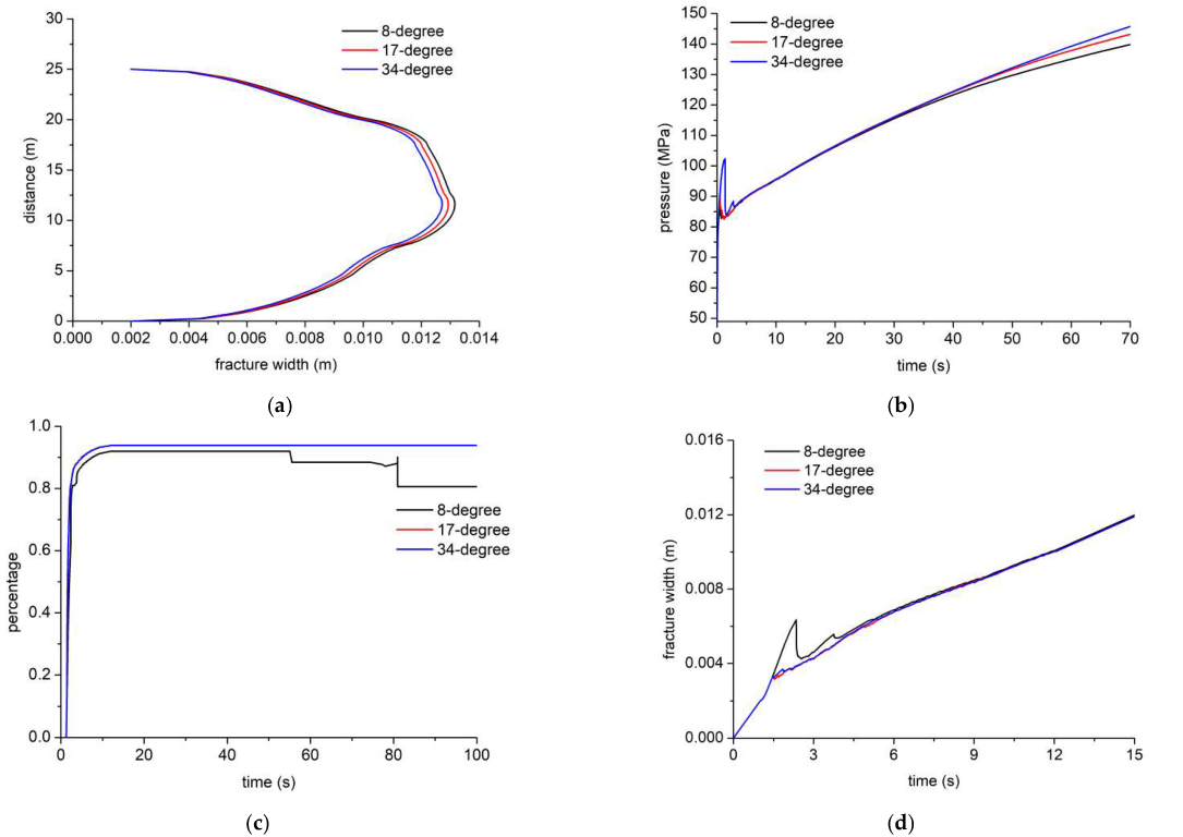
4.2. Effects of Internal Frictional Angle

The internal friction angle is a key parameter in the Mohr–Coulomb criterion for shear failure and determines the rock shear strength. Here, the effects of the internal friction angles of 8°, 17°, and 34° on HF height growth in the layered shale oil reservoir are simulated, respectively.

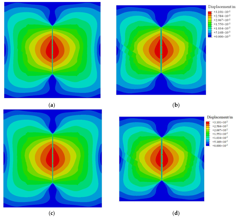
The cloud picture of the displacement field under different internal friction angles is shown in Figure 8. When the internal friction angle of the shale oil reservoir is 8° or 17°, the fracture propagates vertically. When the internal friction angle is 34° (Figure 5f), the HF is diverted and propagates along with the bedding at the later stage. This indicates that as the internal friction angle of the shale oil reservoir decreases, the HF is more likely to propagate vertically along with the cohesive element interface. The HF heights are about 25 m. The value of the displacement field below the injection point is larger than that above, which is caused by the heterogeneous vertical stress profile. In addition, the difference in elastic modulus and Poisson’s ratio of the shell limestone interlayer causes the asymmetric distribution of the displacement field above and below the injection point.

Figure 9 shows the HF width profile, injection pressure, tensile-shear failure ratio, and maximum HF width under different internal friction angles. The larger internal friction angle leads to a smaller HF width (Figure 9a). Especially near the injection point (the ordinate of 12.5 m), there is a large difference in HF width. There is little difference in the HF width profile 5 m away from the injection point, indicating that the internal friction angle mainly affects the HF width near the injection point, and the HF width shows an asymmetric distribution, which is similar to Figure 8. As the internal friction angle increases, the injection pressure increases (Figure 9b). Under the large internal friction angle, the breakdown pressure is about 110 MPa, and when the internal friction angle is low, the breakdown pressure is only about 90 Mpa. There is little difference in breakdown pressure under the internal friction angles of 8° and 17°. In the period of 10 s to 35 s, the injection pressure coincides. After 35 s, the injection pressure increases with the increase of the internal friction angle. This is due to the increase in the internal friction angle requiring more energy for shear failure in the weak interface of the shale oil reservoir. The ratio of tensile failure is higher than 80% (Figure 9c), and HF propagation is dominated by HF height growth. As the internal friction angle is small, the ratio of tensile failure decreases. When the internal friction angle is 8°, the HF width fluctuates (Figure 9d). The reason is possibly due to the shear failure of the vertical cohesive interface. As the injection time increases, the curves of the maximum HF width overlap.

4.3. Effects of Cohesion

Cohesion is also a parameter in the Mohr–Coulomb criterion for shear failure. Here, the effect of cohesion of 8 MPa, 12 MPa, and 17 MPa on HF height growth in the shale oil reservoir is simulated, respectively.

Figure 10 shows the cloud picture of the displacement field under different cohesion values. When the cohesion of the shale oil reservoir is between 8 MPa and 17 MPa, the HF height grows. When the cohesion is 17 MPa, the HF is diverted to the bedding at the late stage (Figure 5f). This indicates that as the cohesion of shale oil reservoir decreases, the HF is more likely to propagate along with the vertical cohesive element interface, and there is a larger difficulty for HF across the bedding interface. The HF height is about 25 m. The displacement field shows an asymmetric distribution below the injection point, which is caused by the heterogeneous stress profile and the difference in mechanical properties of the limestone shell interlayer. In addition, when the cohesion is low, the displacement field presents an elliptical shape in the horizontal direction (marked by black line in Figure 10b). When the cohesion is high, there is no such feature in the horizontal direction of the displacement field in Figure 5f.

Figure 11 shows the HF width profile, injection pressure, tensile-shear failure ratio, and maximum HF width under different cohesion levels. A smaller cohesion value causes a larger HF width (Figure 11a). The HF width profiles are overlapped under the cohesion of 17 Mpa and 12 Mpa and vary significantly when the cohesion is 8 Mpa. The HF width changes rapidly near the injection point, and the HF width profiles overlap far from the injection point, indicating that the cohesion mainly affects the HF width profile near the injection point, and the HF width presents an asymmetric distribution. The HF below the injection point is wider than the HF below, which is consistent with the result in Figure 10. As the cohesion increases, the injection pressure increases (Figure 10b). When the cohesion is high, the breakdown pressure is about 110 Mpa. When the cohesion is low, the breakdown pressure is only about 90 Mpa. The injection pressure curves vary significantly. The higher cohesion causes the higher injection pressure. The increased cohesion requires more energy for HF initiation. The ratio of tensile failure is higher than 80% (Figure 11c), indicating that HF propagation is dominated by tensile failure and HF height growth. When the cohesion is small, the ratio of tensile failure decreases. When the cohesion is 8 Mpa, the HF width fluctuates at the initial stage (Figure 11d), which is caused by the shear failure of the vertical cohesive interface. As the injection of fracture fluid goes on, the curves of the maximum HF width basically overlap.

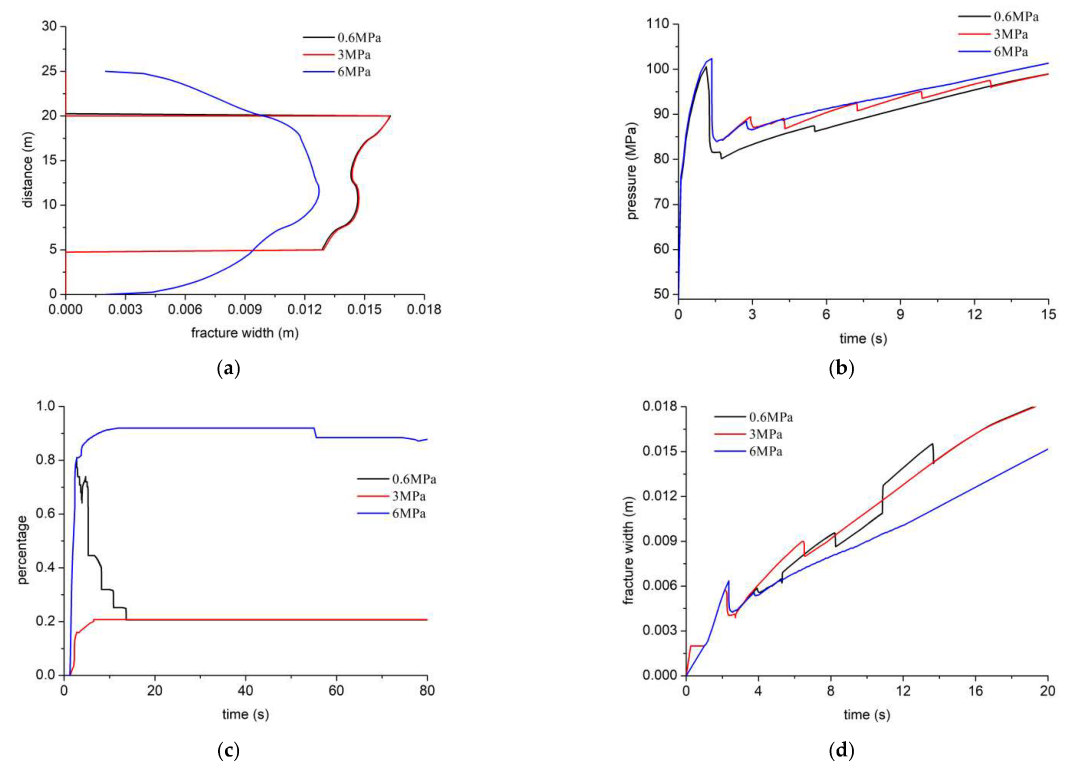
4.4. Effects of Bedding Bond Strength

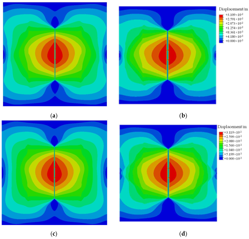
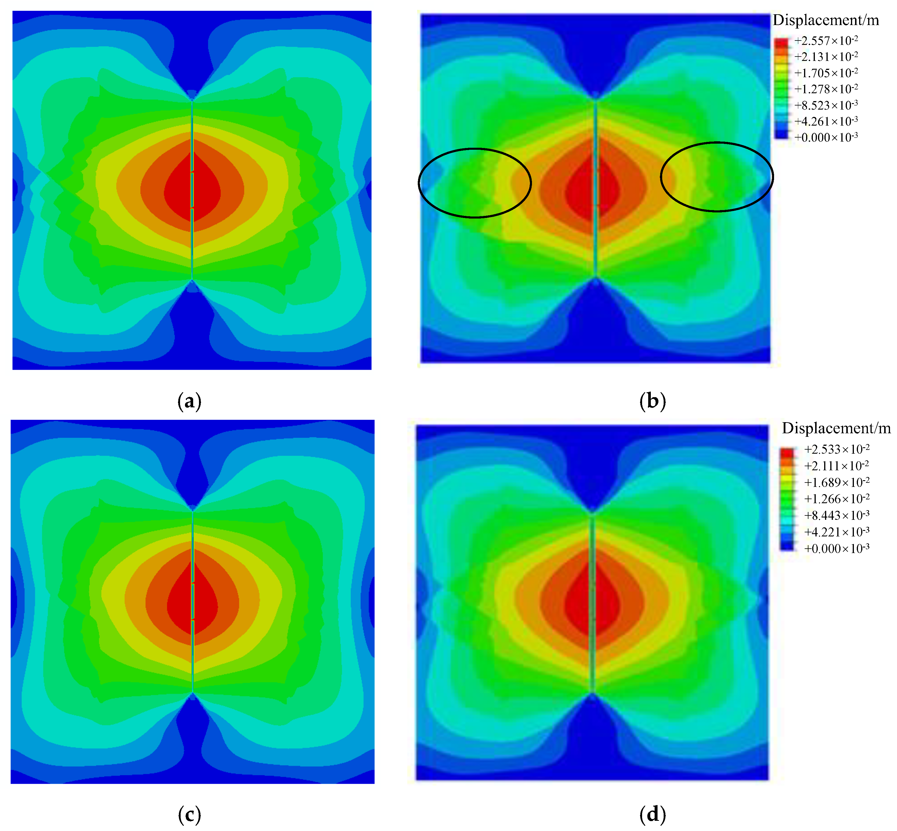
The bedding is filled with various materials and is classified as high electrical resistivity fractures and low electrical resistivity fractures in logging interpretation, which show different pressure responses in hydraulic fracturing. The effect of bedding bond strength on HF propagation in the shale oil reservoir is simulated here.

Figure 12 shows the cloud picture of the displacement field under bond strength corresponding to low electrical resistivity fracture (0.6 MPa), medium electrical resistivity fracture (3 Mpa), and high electrical resistivity fracture (6 Mpa, base case). When the bedding bond strength is low, the HF is likely to be diverted to the bedding (Figure 12a–d), and the HF height is about 15 m. When the bedding bond strength is high (Figure 5e,f), the HF height grows vertically, and the HF height increases by about 10 m. The value of the displacement field above the injection point is larger than the below and shows an asymmetric distribution.

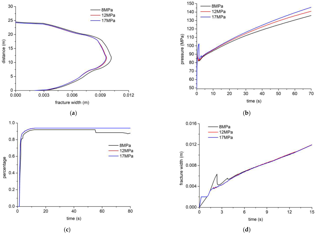
Figure 13 shows HF width profile, injection pressure, tensile-shear failure ratio, and maximum HF width under different bedding bonding strengths. Figure 13a shows the HF width profile. The HF width profiles across both low and high electrical resistivity bedding coincide. The fracture above the injection point is wider than that below the injection point. There is a large difference in HF width profile of the high electrical resistivity bedding. The HF height across the high electrical resistivity bedding is about 10 m more than that across the medium and low electrical resistivity bedding, which is similar to the result in Figure 12. The injection pressure curve fluctuates more frequently under the medium and low electrical resistivity bedding than under the high electrical resistivity bedding (Figure 13b). This is due to the fact that interaction between HF and the medium and low electrical resistivity bedding is likely to occur, and the typical pressure response for the complex fracture network is formed. The breakdown pressure of high-electrical-resistivity bedding is about 3 Mpa higher than that of the medium and low-electrical-resistivity bedding. Figure 13c shows the proportion of tensile failure. The tensile failure ratio of medium and low electrical resistivity bedding is only about 20%, indicating that the interaction between HF and bedding is dominated by shear failure. The tensile failure ratio is more than 80% in the high-electrical-resistivity bedding, and the HF propagates vertically and is dominated by tensile failure. There is a significant difference in the maximum HF height (Figure 13d) and the HF width increases as the bedding bond strength increases.

4.5. Effects of Elastic Modulus

The layers in the shale oil reservoir vary significantly in the lithology and mechanical properties including elastic modulus. The effects of the elastic modulus on the HF height growth are simulated here.

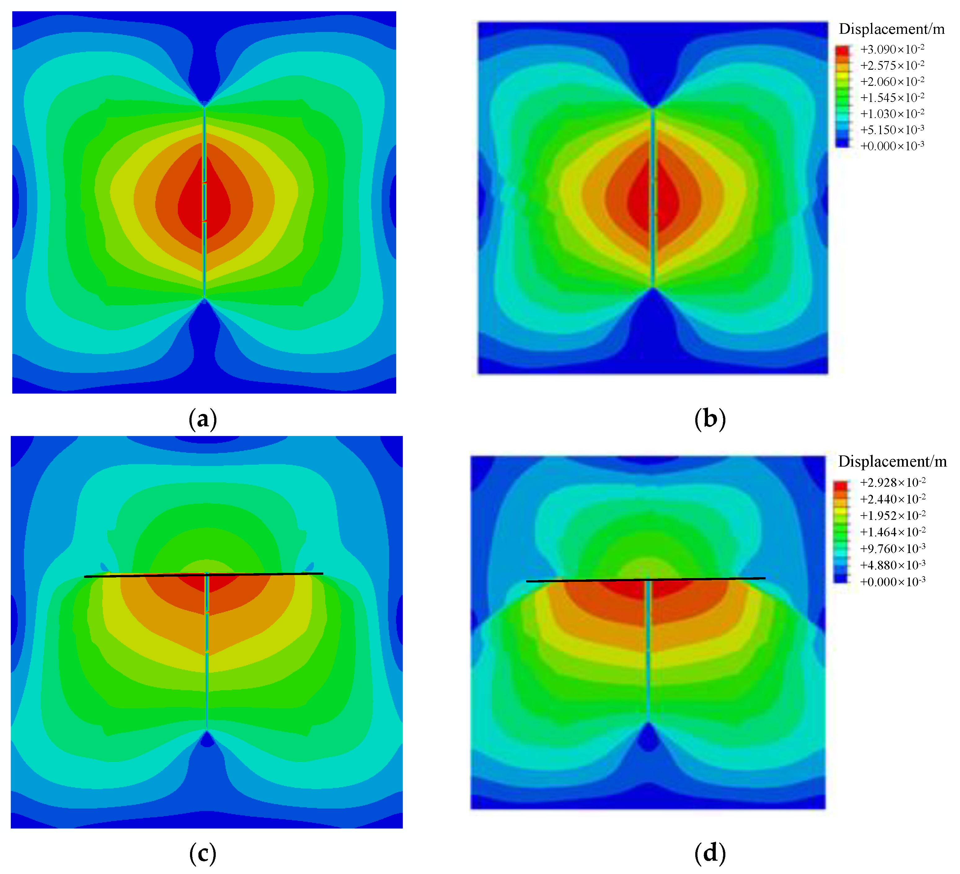
Figure 14 shows the cloud picture of the displacement field when the elastic modulus of the No. 4 layer is 25 GPa, 35 Gpa, and 45 Gpa, respectively. When the elastic modulus is 45 Gpa (Figure 14c,d), the HF height hardly grows. The layer with high elastic modulus restricts HF height growth, and the HF is diverted to and propagates along with the bedding, which is marked by the black line. The low elastic modulus has a weak restriction on HF height growth and is favorable for hydraulic fracture across more layers.

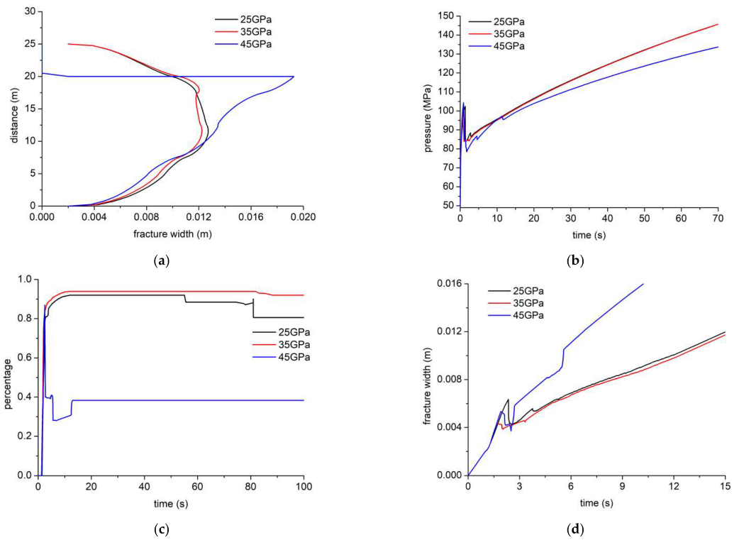
Figure 15 shows HF width profile, injection pressure, tensile-shear failure ratio, and maximum HF width under different elastic moduli of layers. There is a large difference in the HF width profile (Figure 15a). The high-elastic modulus layer restricts HF height growth, and the HF is diverted to bedding between No. 4 and No. 5 layers. When the layer elastic modulus is 25 Gpa and 35 Gpa, the HF height is all about 25 m, and the HF width increases slightly when the elastic modulus is 35 Gpa, especially near the injection point. The HF width coincides far away from the injection point. The injection pressure decreases as the injection pressure increases (Figure 15b). The injection pressure curves overlap when the elastic modulus is 25 Gpa and 35 Gpa. When the elastic modulus is 45 Gpa, the injection pressure fluctuates initially, and the breakdown pressure also increases. Under the high layer elastic modulus (Figure 15c), the ratio of tensile failure is about 40%, and HF propagation is dominated by shear failure. The HF is diverted to the bedding. When the layer elastic modulus is 25 Gpa and 35 Gpa, the ratio of tensile failure is more than 80%, and HF propagation is dominated by vertical growth and tensile failure. As the elastic modulus of the No. 4 layer increases, the maximum HF width increases (Figure 15d). The HF width fluctuates due to more energy being required for opening the bedding and HF being diverted to the bedding. When maximum HF width decreases as the elastic modulus decreases from 35 Gpa to 25 GP. After 6 s of injection, the difference in the maximum fracture decreases.

4.6. Effects of Layered Stress Contrast

The shale oil reservoir is characterized by strong vertical lithological heterogeneity, large stress contrast, and a non-uniform distribution of principal stress differences between sublayers. Here, the effect of longitudinal stress contrast between layers on HF height growth is simulated. The stress contrast between No. 2 layer and No. 2 shell limestone layer is set as 4 MPa (base case), 6 Mpa, and 8 Mpa.

Figure 16 shows the cloud picture of the displacement field under different layered stress contrasts. As the layered stress contrast increases, the difficulty in HF growth across the layered shale oil reservoirs increases accordingly and the HF is diverted to and propagates along with the bedding. The displacement field above and below the opened bedding interface is differentiated and shows the typical asymmetric distribution. The vertical HF height is about 25 m, indicating that the layered stress contrast restricts vertical HF propagation in the shale oil reservoir. After the stress contrast is overcome, the HF still grows vertically.

Figure 17 shows the HF width profile, injection pressure, tensile-shear failure ratio, and maximum HF width under different longitudinal stress contrast levels. The HF width decreases (Figure 17a) when the layered stress contrast increases, especially when the stress contrast reaches 8 Mpa. The injection pressure curves overlap (Figure 17b). The ratio of tensile failure reaches 80% (Figure 17c), and HF propagation is dominated by tensile failure. The layered stress contrast has a certain restriction effect on the HF height at the early stage of injection. When the HF height breaks through the layer with the high stress contrast, the HF height still grows. When the injection time is less than 9 s, the maximum HF width increases as the stress contrast increases (Figure 17d), and more energy is needed to overcome the layered stress contrast. After 9 s of injection, the maximum HF width profile coincides, the HF height continues to grow vertically, and the maximum HF width is less disturbed by the layered stress contrast.

4.7. Effects of Injection Rate

The injection rate is a key parameter in HF height growth in the layered shale oil reservoir. The effects of injection rates of 3 m³/min, 6 m³/min, and 12 m³/min are simulated. The HF height propagation across the shale oil reservoir is simulated, respectively.

Figure 18 shows the cloud picture of the displacement field under displacement. The higher displacement promotes HF height growth across the shale oil reservoir, and the displacement field shows a symmetrical distribution under the low rate. Under the high injection rate, the displacement field shows an asymmetric distribution.

Figure 19 shows the HF width profile, injection pressure, tensile-shear failure ratio, and maximum HF width under different injection rates. As the injection rate increases, the HF width increases (Figure 19a), and its asymmetric distribution is enhanced. The vertical HF propagation distance under the injection rate of 12 m³/min is five times that under the injection rate of 3 m³/min. The result is similar to Figure 18. The HF height is about 25 m, 10 m, and 5 m under the injection rate of 12 m³/min, 6 m³/min, and 3 m³/min, respectively. The injection pressure increases with the increase of the injection rate (Figure 19b). When the injection rate is 12 m³/min, the breakdown pressure is about 100 MPa, and the injection pressure gradually increases. When the injection rate is 6 m³/min and 3 m³/min, the breakdown pressure is about 85 Mpa, and the injection pressure is stabilized at about 85 Mpa. As the injection rate increases, the ratio of tensile failure increases (Figure 19c). When the injection rate is 6 m³/min and 3 m³/min, the ratio of tensile failure is about 40%, showing a mixture of tensile-shear failure. The maximum HF width increases with the injection rate (Figure 19d). Under the high injection rate, the maximum HF width fluctuates initially and then increases. When the injection rate is 6 m³/min and 3 m³/min, the maximum HF width has little difference.

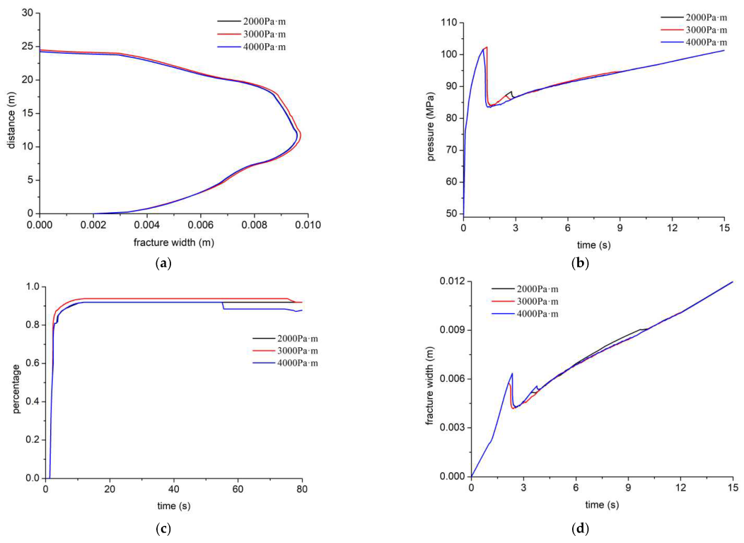
4.8. Effects of Fracture Energy

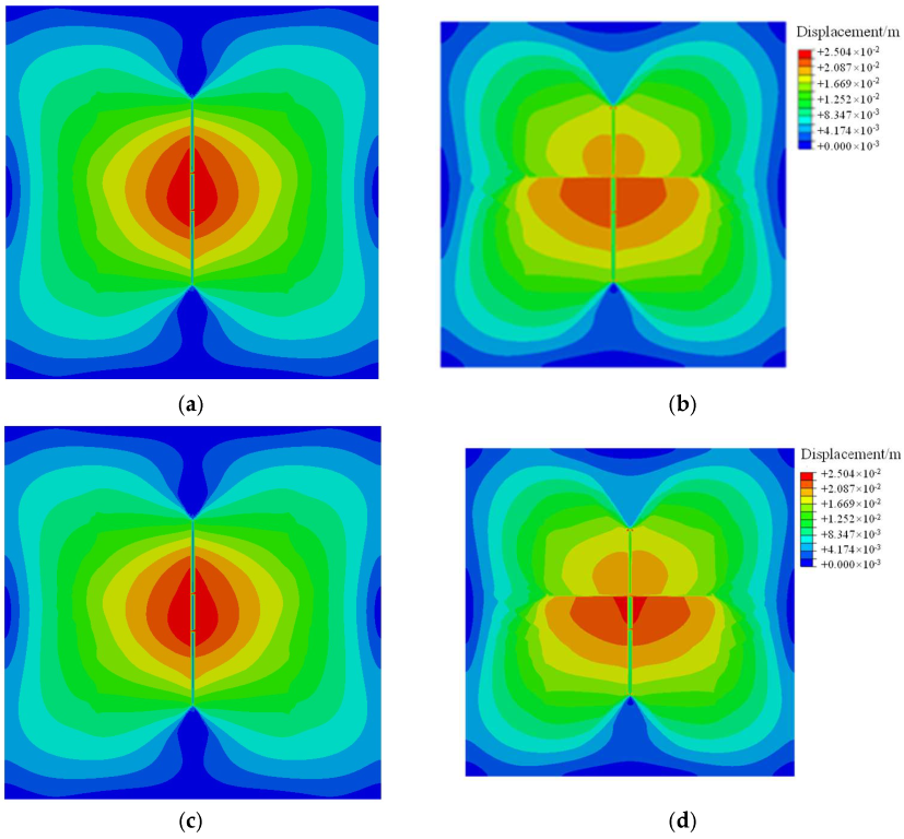
Fracture toughness is a key parameter in HF height growth in the shale oil reservoirs, and it is transferred to the fracture energy through the Irwin formula. Here, the effect of the fracture energy of 2000 Pa·m, 3000 Pa·m, and 4000 Pa·m on HF propagation is simulated, respectively.

Figure 20 shows the cloud picture of the displacement field under different fracture energies. The HF propagates vertically and is not diverted to the bedding. The displacement field under the fracture energy of 3000 Pa·m and 4000 Pa·m has little difference (Figure 20a–d). When the fracture energy is 2000 Pa·m (Figure 5f), the HF is diverted to the bedding at a later stage. The bedding with low fracture energy is opened under the action of certain fluid pressure.

Figure 21 shows the HF width profile, injection pressure, tensile failure ratio, and maximum HF width under different fracture energies. There is little difference in the HF width profile (Figure 21a), and the HF width is only slightly different near the injection point. There is little difference in the injection pressure curve (Figure 21b). When the fracture energy is low, the injection pressure fluctuates slightly. The ratio of tensile failure is more than 80% (Figure 21c). The HF propagates vertically and is hardly diverted to the bedding. When the fracture energy is 4000 Pa·m, the maximum HF width is larger initially (Figure 21d).

5. Conclusions

This paper used the cohesive zone method to establish an elastic–plastic finite element model for HF height growth in shale oil reservoirs by considering the shell limestone interlayer, the Mohr–Coulomb criterion for tensile and shear failure, the cross-mechanical interaction between bedding and shale oil reservoir, HF growth across high-electrical resistivity and high-conduction bedding, and the effects of internal friction angle, cohesion, layered stress contrast, fracture toughness, bedding bond strength, injection rate, elastic modulus, and bedding shear strength on HF height growth were simulated, respectively. The HF width profile, injection pressure, failure mode, and maximum HF width was discussed in detail. The main conclusions are as follows.

(1) Compared with the layered stress contrast, cohesion, internal friction angle, and fracture toughness, injection rate, elastic modulus, bedding shear strength, and bedding bond strength have a larger effect on the HF width profile, especially near the injection point. A decrease in the injection rate, bedding shear strength and bedding bond strength are favorable for and bedding bond strength are favorable for HF growth across more layers in the shale oil reservoir.

(2) The layered stress contrast has a certain restriction effect on the HF height growth at the initial stage. After a certain time of injection, the layered stress difference is overcome, and the HF still grows vertically. The layered stress contract has little effect on the HF width profile, injection pressure, maximum HF width, etc.

(3) When the high-conductivity bedding exists, the HF is likely to be diverted to and propagate along with the bedding, HF height growth is very difficult. The HF propagation is dominated by the mechanical mechanism of shear failure. The injection pressure and the maximum HF width fluctuate, which is caused by the interaction between HF and the bedding. HF propagation in the high-electric-resistivity bedding is dominated by tensile failure, and the injection pressure and maximum HF width increase and fluctuate slightly as fracturing operation goes on. The high-electric resistivity-bedding helps HF height growth.

(4) Cohesion and internal friction angle are the key elastic–plastic parameters in HF growth in shale oil reservoirs. A higher cohesion and internal friction angle causes a smaller HF width, which increases the risk of proppant plugging during hydraulic fracturing, and the maximum HF height and injection pressure fluctuate, which are caused by shear failure. To a certain extent, the tensile failure mode during HF propagation is weakened under the lower cohesion and internal friction angle. As the cohesion and the internal friction angle increase, the injection pressure increases, and HF propagation across the layers requires more energy.

(5) The layer with the high elastic modulus provides an interlayer for restricting HF height growth and enhancing HF diversion to the bedding. The shell limestone interlayer is a negative factor in HF height growth in shale oil reservoirs. It is recommended to apply a high injection rate to overcome the adverse effects caused by the high elastic modulus of layers.

(6) The elastic–plastic finite element model of fracture height growth is a 2D model and does not consider fracture length propagation. In this paper, we assume the intersection angle of 90° between fracture height and bedding planes. The case of inclined angle is worth studying in future works.