
Comparison Process of Blood Heavy Metals Absorption Linked to Measured Air Quality Data in Areas with High and Low Environmental Impact

 ,
,  , ,
, ,  ,
,  and
and 
Abstract
:1. Introduction
2. Materials and Methods
2.1. Participants
2.2. Heavy Metals Procedure to Assess the Blood Concentration
2.3. Air Quality
2.4. Pollutant Adsorption
- Ci is the contaminant concentration measured, [μg/m3];
- IR is the inhalation rate [m3/h];
- BW is the body weight [kg];
- ET is the exposure time [h/day];
- EF is the exposure frequency [days/year];
- ED is the exposure duration [years]
- AT is the averaging time [days].
3. Results and Discussion
3.1. Heavy Metals Blood Concentrations
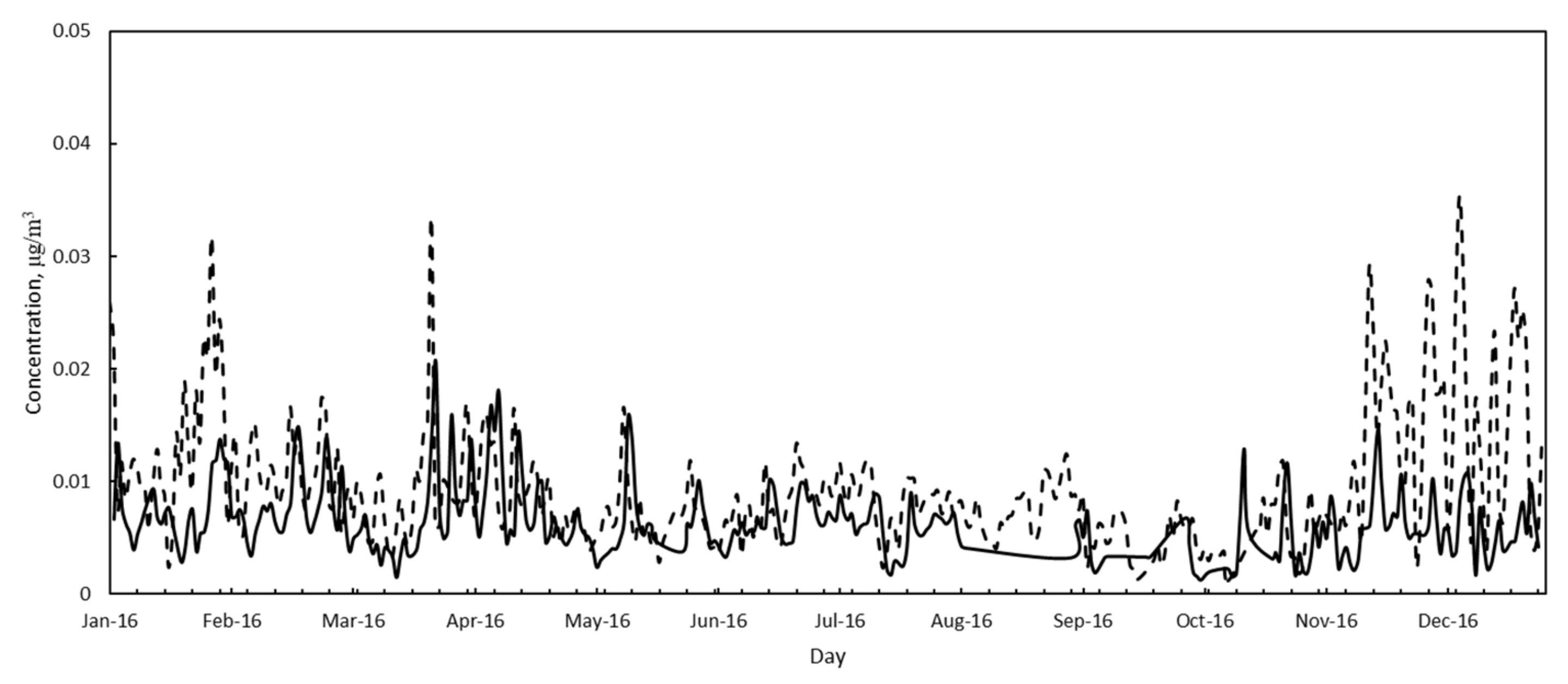
3.2. Air Quality
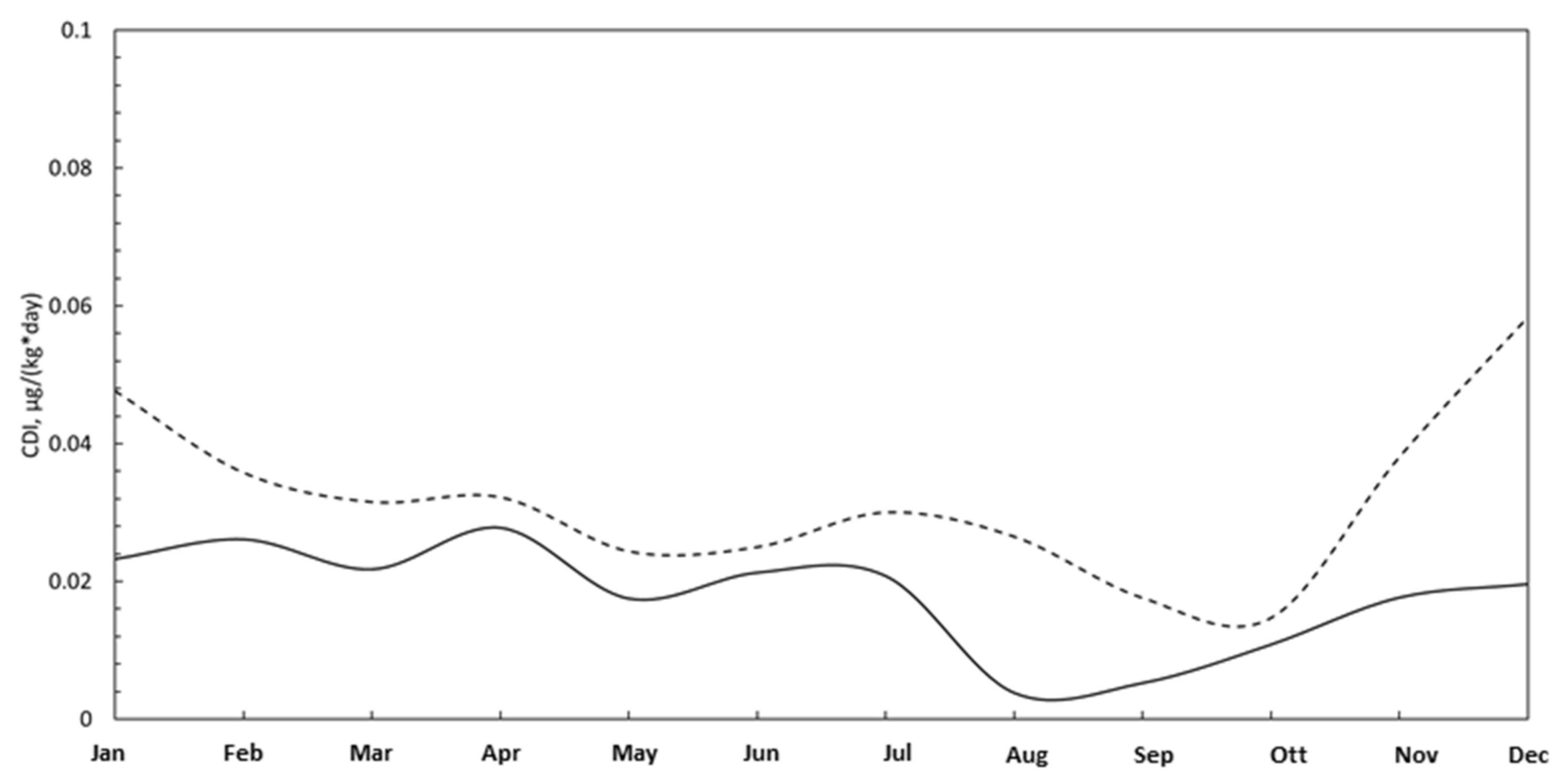
3.3. Pollutants Adsorption
4. Conclusions
Author Contributions
Funding
Institutional Review Board Statement
Informed Consent Statement
Data Availability Statement
Acknowledgments
Conflicts of Interest
References
- European Environment Agency (EEA). Healthy Environment, Healthy Lives: How the Environment Influences Health and Well-Being in Europe; Publications Office: Luxembourg, 2020. [Google Scholar] [CrossRef]
- Lim, S.S.; Vos, T.; Flaxman, A.D.; Danaei, G.; Shibuya, K.; Adair-Rohani, H.; Amann, M.; Anderson, H.R.; Andrews, K.G.; Aryee, M.; et al. A comparative risk assessment of burden of disease and injury attributable to 67 risk factors and risk factor clusters in 21 regions, 1990–2010: A systematic analysis for the Global Burden of Disease Study 2010. Lancet 2012, 380, 2224–2260. [Google Scholar] [CrossRef] [Green Version]
- Cohen, A.J.; Anderson, H.R.; Ostro, B.; Pandey, K.V.; Krzyzanowski, M.; Künzli, N.; Gutschmidt, K.; Pope, A.; Romieu, I.; Samet, J.M.; et al. The Global Burden of Disease due to Outdoor Air Pollution. J. Toxicol. Environ. Health A 2005, 68, 1301–1307. [Google Scholar] [CrossRef] [PubMed]
- Ezzati, M.; Lopez, A.D.; Rodgers, A.; Vander Hoorn, S.; Murray, C.J. Selected major risk factors and global and regional burden of disease. Lancet 2002, 360, 1347–1360. [Google Scholar] [CrossRef]
- Krewski, D.; Jerrett, M.; Burnett, R.T.; Ma, R.; Hughes, E.; Shi, Y.; Turner, M.C.; Pope, C.A., 3rd; Thurston, G.; Calle, E.E.; et al. Extended Follow-Up and Spatial Analysis of the American Cancer Society Study Linking Particulate Air Pollution and Mortality. Res. Rep. Health Eff. Inst. 2009, 140, 5–114; discussion 115. [Google Scholar]
- Pope, C.A.; Ezzati, M.; Dockery, D.W. Fine-Particulate Air Pollution and Life Expectancy in the United States. N. Engl. J. Med. 2009, 360, 376–386. [Google Scholar] [CrossRef] [Green Version]
- Laden, F.; Schwartz, J.; Speizer, F.; Dockery, D. Reduction in Fine Particulate Air Pollution and Mortality: Extended Follow-up of the Harvard Six Cities Study. Am. J. Respir. Crit. Care Med. 2006, 173, 667–672. [Google Scholar] [CrossRef] [Green Version]
- Kim, D.; Chen, Z.; Zhou, L.-F.; Huang, S.-X. Air pollutants and early origins of respiratory diseases. Spec. Issue Air Pollut. Chronic Respir. Dis. 2018, 4, 75–94. [Google Scholar] [CrossRef]
- Mitova, M.I.; Cluse, C.; Goujon-Ginglinger, C.G.; Kleinhans, S.; Rotach, M.; Tharin, M. Human chemical signature: Investigation on the influence of human presence and selected activities on concentrations of airborne constituents. Environ. Pollut. 2020, 257, 113518. [Google Scholar] [CrossRef]
- Cambra-López, M.; Aarnink, A.J.A.; Zhao, Y.; Calvet, S.; Torres, A.G. Airborne particulate matter from livestock production systems: A review of an air pollution problem. Environ. Pollut. 2010, 158, 1–17. [Google Scholar] [CrossRef]
- Hsu, A.; Reuben, A.; Shindell, D.; de Sherbinin, A.; Levy, M. Toward the next generation of air quality monitoring indicators. Atmos. Environ. 2013, 80, 561–570. [Google Scholar] [CrossRef] [Green Version]
- Whelpdale, D.M. Particulate residence times. Water. Air. Soil Pollut. 1974, 3, 293–300. [Google Scholar] [CrossRef]
- Anderson, J.O.; Thundiyil, J.G.; Stolbach, A. Clearing the Air: A Review of the Effects of Particulate Matter Air Pollution on Human Health. J. Med. Toxicol. 2012, 8, 166–175. [Google Scholar] [CrossRef] [Green Version]
- Kim, K.-H.; Kabir, E.; Kabir, S. A review on the human health impact of airborne particulate matter. Environ. Int. 2015, 74, 136–143. [Google Scholar] [CrossRef]
- Hussain, S.; Rengel, Z.; Qaswar, M.; Amir, M.; Zafar-ul-Hye, M. Arsenic and Heavy Metal (Cadmium, Lead, Mercury and Nickel) Contamination in Plant-Based Foods. In Plant and Human Health, Volume 2: Phytochemistry and Molecular Aspects; Ozturk, M., Hakeem, K.R., Eds.; Springer International Publishing: Cham, Switzerland, 2019; pp. 447–490. [Google Scholar] [CrossRef]
- Sun, Z.; Zhu, D. Exposure to outdoor air pollution and its human health outcomes: A scoping review. PLoS ONE 2019, 14, e0216550. [Google Scholar] [CrossRef]
- Satarug, S.; Gobe, G.C.; Vesey, D.A.; Phelps, K.R. Cadmium and lead exposure, nephrotoxicity, and mortality. Toxics 2020, 8, 86. [Google Scholar] [CrossRef]
- Alengebawy, A.; Abdelkhalek, S.T.; Qureshi, S.R.; Wang, M.-Q. Heavy metals and pesticides toxicity in agricultural soil and plants: Ecological risks and human health implications. Toxics 2021, 9, 42. [Google Scholar] [CrossRef]
- Massányi, P.; Massányi, M.; Madeddu, R.; Stawarz, R.; Lukáč, N. Effects of cadmium, lead, and mercury on the structure and function of reproductive organs. Toxics 2020, 8, 94. [Google Scholar] [CrossRef]
- Satarug, S. Dietary cadmium intake and its effects on kidneys. Toxics 2018, 6, 15. [Google Scholar] [CrossRef] [Green Version]
- Sijko, M.; Kozłowska, L. Influence of dietary compounds on arsenic metabolism and toxicity. Part i—Animal model studies. Toxics 2021, 9, 258. [Google Scholar] [CrossRef]
- Silvera, S.A.N.; Rohan, T.E. Trace elements and cancer risk: A review of the epidemiologic evidence. Cancer Causes Control. 2007, 18, 7–27. [Google Scholar] [CrossRef]
- Sofia, D.; Giuliano, A.; Gioiella, F. Air quality monitoring network for tracking pollutants: The case study of salerno city center. Chem. Eng. Trans. 2018, 68, 67–72. [Google Scholar] [CrossRef]
- Sofia, D.; Lotrecchiano, N.; Trucillo, P.; Giuliano, A.; Terrone, L. Novel air pollution measurement system based on ethereum blockchain. J. Sens. Actuator Netw. 2020, 9, 49. [Google Scholar] [CrossRef]
- Sofia, D.; Lotrecchiano, N.; Giuliano, A.; Barletta, D.; Poletto, M. Optimization of number and location of sampling points of an air quality monitoring network in an urban contest. Chem. Eng. Trans. 2019, 74, 277–282. [Google Scholar] [CrossRef]
- Lotrecchiano, N.; Sofia, D.; Giuliano, A.; Barletta, D.; Poletto, M. Spatial Interpolation Techniques For innovative Air Quality Monitoring Systems. Chem. Eng. Trans. 2021, 86, 391–396. [Google Scholar] [CrossRef]
- Lotrecchiano, N.; Gioiella, F.; Giuliano, A.; Sofia, D. Forecasting Model Validation of Particulate Air Pollution by Low Cost Sensors Data. J. Model. Optim. 2019, 11, 63–68. [Google Scholar] [CrossRef] [Green Version]
- Lotrecchiano, N.; Sofia, D.; Giuliano, A.; Barletta, D.; Poletto, M. Pollution dispersion from a fire using a Gaussian plume model. Int. J. Saf. Secur. Eng. 2020, 10, 431–439. [Google Scholar] [CrossRef]
- Sofia, D.; Gioiella, F.; Lotrecchiano, N.; Giuliano, A. Mitigation strategies for reducing air pollution. Environ. Sci. Pollut. Res. 2020, 27, 19226–19235. [Google Scholar] [CrossRef] [PubMed]
- Sofia, D.; Gioiella, F.; Lotrecchiano, N.; Giuliano, A. Cost-benefit analysis to support decarbonization scenario for 2030: A case study in Italy. Energy Policy 2020, 137, 111137. [Google Scholar] [CrossRef]
- Kunugi, Y.; Arimura, T.H.; Iwata, K.; Komatsu, E.; Hirayama, Y. Cost-efficient strategy for reducing PM 2.5 levels in the Tokyo metropolitan area: An integrated approach with air quality and economic model. PLoS ONE 2018, 13, e0207623. [Google Scholar] [CrossRef] [PubMed]
- Singh, V.; Meena, K.K.; Agarwal, A. Travellers’ exposure to air pollution: A systematic review and future directions. Urban Clim. 2021, 38, 100901. [Google Scholar] [CrossRef]
- Hormigos-Jimenez, S.; Padilla-Marcos, M.Á.; Meiss, A.; Gonzalez-Lezcano, R.A.; Feijó-Muñoz, J. Assessment of the ventilation efficiency in the breathing zone during sleep through computational fluid dynamics techniques. J. Build. Phys. 2019, 42, 458–483. [Google Scholar] [CrossRef]
- Becerra, J.A.; Lizana, J.; Gil, M.; Barrios-Padura, A.; Blondeau, P.; Chacartegui, R. Identification of potential indoor air pollutants in schools. J. Clean. Prod. 2020, 242, 118420. [Google Scholar] [CrossRef]
- Mendes, A.; Bonassi, S.; Aguiar, L.; Pereira, C.; Neves, P.; Silva, S.; Teixeira, J.P. Indoor air quality and thermal comfort in elderly care centers. Urban Clim. 2015, 14, 486–501. [Google Scholar] [CrossRef] [Green Version]
- Environmental Protection Agency (EPA). Proposed Guidelines for Exposure-Related Measurements; Federal Register: Washington, DC, USA, 1988.
- Ott, W.R. Total human exposure. Environ. Sci. Technol. 1985, 19, 880–885. [Google Scholar] [CrossRef]
- Sexton, K.; Barry Ryan, P. Assessment of Humen Exposure to Air Pollution: Methods, Measurements, and Models. In Air Pollution, the Automobile, and Public Health; Health Effects Institute, National Academy Press: Washington, DC, USA, 1988. [Google Scholar]
- Asante-Duah, K. Exposure Assessment: Analysis of Human Intake of Chemicals. In Public Health Risk Assessment for Human Exposure to Chemicals; Asante-Duah, K., Ed.; Springer: Dordrecht, The Netherlands, 2017; pp. 189–229. [Google Scholar] [CrossRef]
- Triassi, M.; Alfano, R.; Illario, M.; Nardone, A.; Caporale, O.; Montuori, P. Environmental Pollution from Illegal Waste Disposal and Health Effects: A Review on the “Triangle of Death”. Int. J. Environ. Res. Public. Health 2015, 12, 1216–1236. [Google Scholar] [CrossRef] [PubMed] [Green Version]
- Maisto, G.; Baldantoni, D.; De Marco, A.; Alfani, A.; Virzo De Santo, A. Biomonitoring of trace element air contamination at sites in Campania (Southern Italy). J. Trace Elem. Med. Biol. 2003, 7 (Suppl. 1), 51–55. [Google Scholar]
- Posters. Andrology 2014, 2, 45–117. [CrossRef]
- Pacini, N.; Abate, V.; Brambilla, G.; De Felip, E.; De Filippis, S.P.; De Luca, S.; di Domenico, A.; D’Orsi, A.; Forte, T.; Fulgenzi, A.R.; et al. Polychlorinated dibenzodioxins, dibenzofurans, and biphenyls in fresh water fish from Campania Region, southern Italy. Chemosphere 2013, 90, 80–88. [Google Scholar] [CrossRef]
- EcoFoodFertility project. Available online: http://www.ecofoodfertility.it/the-project.html. (accessed on 18 January 2021).
- Montano, L.; Iannuzzi, L.; Rubes, J.; Avolio, C.; Pistos, C.; Gatti, A.; Raimondo, S.; Notari, T. EcoFoodFertility—Environmental and food impact assessment on male reproductive function. Andrology 2014, 2 (Suppl. 2), 69. [Google Scholar]
- World Medical Association. World Medical Association Declaration of Helsinki: Ethical Principles for Medical Research Involving Human Subjects. JAMA 2013, 310, 2191–2194. [Google Scholar] [CrossRef] [Green Version]
- Vecoli, C.; Montano, L.; Borghini, A.; Notari, T.; Guglielmino, A.; Mercuri, A.; Turchi, S.; Andreassi, M.G. Effects of Highly Polluted Environment on Sperm Telomere Length: A Pilot Study. Int. J. Mol. Sci. 2017, 18, 1703. [Google Scholar] [CrossRef] [Green Version]
- Montano, L.; Ceretti, E.; Donato, F.; Bergamo, P.; Zani, C.; Viola, G.; Notari, T.; Pappalardo, S.; Zani, D.; Ubaldi, S.; et al. Effects of a Lifestyle Change Intervention on Semen Quality in Healthy Young Men Living in Highly Polluted Areas in Italy: The FASt Randomized Controlled Trial. Eur. Urol. Focus 2022, 8, 351–359. [Google Scholar] [CrossRef]
- Lettieri, G.; D’Agostino, G.; Mele, E.; Cardito, C.; Esposito, R.; Cimmino, A.; Giarra, A.; Trifuoggi, M.; Raimondo, S.; Notari, T.; et al. Discovery of the Involvement in DNA Oxidative Damage of Human Sperm Nuclear Basic Proteins of Healthy Young Men Living in Polluted Areas. Int. J. Mol. Sci. 2020, 21, 4198. [Google Scholar] [CrossRef]
- Bosco, L.; Notari, T.; Ruvolo, G.; Roccheri, M.C.; Martino, C.; Chiappetta, R.; Carone, D.; Lo Bosco, G.; Carrillo, L.; Raimondo, S.; et al. Sperm DNA fragmentation: An early and reliable marker of air pollution. Environ. Toxicol. Pharmacol. 2018, 58, 243–249. [Google Scholar] [CrossRef]
- Longo, V.; Forleo, A.; Ferramosca, A.; Notari, T.; Pappalardo, S.; Siciliano, P.; Capone, S.; Montano, L. Blood, urine and semen Volatile Organic Compound (VOC) pattern analysis for assessing health environmental impact in highly polluted areas in Italy. Environ. Pollut. 2021, 286, 117410. [Google Scholar] [CrossRef]
- Senior, K.; Mazza, A. Italian “Triangle of death” linked to waste crisis. Lancet Oncol. 2004, 5, 525–527. [Google Scholar] [CrossRef]
- US Environmental Protecgtion Agency (EPA). Users’ Guide and Background Technical Document for USEPA Region 9—Preliminary Remediation Goals (PRG) Table. 2013. Available online: https://semspub.epa.gov/work/02/103453.pdf (accessed on 30 April 2021).
- I International Commission on Radiological Protection (ICRP). Human Respiratory Tract Model for Radiological Protection. A report of a Task Group of the International Commission on Radiological Protection. Ann. ICRP 2002, 32, 307–309. [Google Scholar]
- US Environmental Protecgtion Agency (EPA). Risk Assessment Guidance for Superfund, Volume I: Human Health Evaluation Manual (Part A); Environmental Protection Agency: Washington, DC, USA, 1989.
- US Environmental Protecgtion Agency (EPA). Risk Assessment Guidance for Superfund Volume I: Human Health Evaluation Manual (Part F, Supplemental Guidance for Inhalation Risk Assessment); Environmental Protection Agency: Washington, DC, USA, 2003.
- Alimonti, A.; Bocca, B.; Mattei, D.; Pino, A. Biomonitoraggio della popolazione italiana per l’esposizione ai metalli: Valori di riferimento 1990–2009. Rapp. Istisan-Ist. Super. Di Sanità 2010, 10, 58. [Google Scholar]
- Elinder, C.G.; Järup, L. Cadmium Exposure and Health Risks: Recent Findings. Ambio 1996, 25, 370–373. [Google Scholar]
- Baralić, K.; Javorac, D.; Marić, D.; Đukić-Ćosić, D.; Bulat, Z.; Antonijević Miljaković, E.; Anđelković, M.; Antonijević, B.; Aschner, M.; Buha Djordjevic, A. Benchmark dose approach in investigating the relationship between blood metal levels and reproductive hormones: Data set from human study. Environ. Int. 2022, 165, 107313. [Google Scholar] [CrossRef]
- Magnano, G.C.; Marussi, G.; Pavoni, E.; Adami, G.; Larese Filon, F.; Crosera, M. Percutaneous metals absorption following exposure to road dust powder. Environ. Pollut. 2022, 292, 118353. [Google Scholar] [CrossRef] [PubMed]
- Chen, Y.; Luo, X.-S.; Zhao, Z.; Chen, Q.; Wu, D.; Sun, X.; Wu, L.; Jin, L. Summer–winter differences of PM2.5 toxicity to human alveolar epithelial cells (A549) and the roles of transition metals. Ecotoxicol. Environ. Saf. 2018, 165, 505–509. [Google Scholar] [CrossRef] [PubMed]


| LI Area | HI Area | |
|---|---|---|
| Number of male participants | 35 | 40 |
| Age, years | 30 | 28 |
| Weight, kg | 78 | 77 |
| Height, m | 1.77 | 1.76 |
| BMI | 24.6 | 25 |
| Average Concentration, μg/L | 95% CI | |||
|---|---|---|---|---|
| LI Area | HI Area | LI Area | HI Area | |
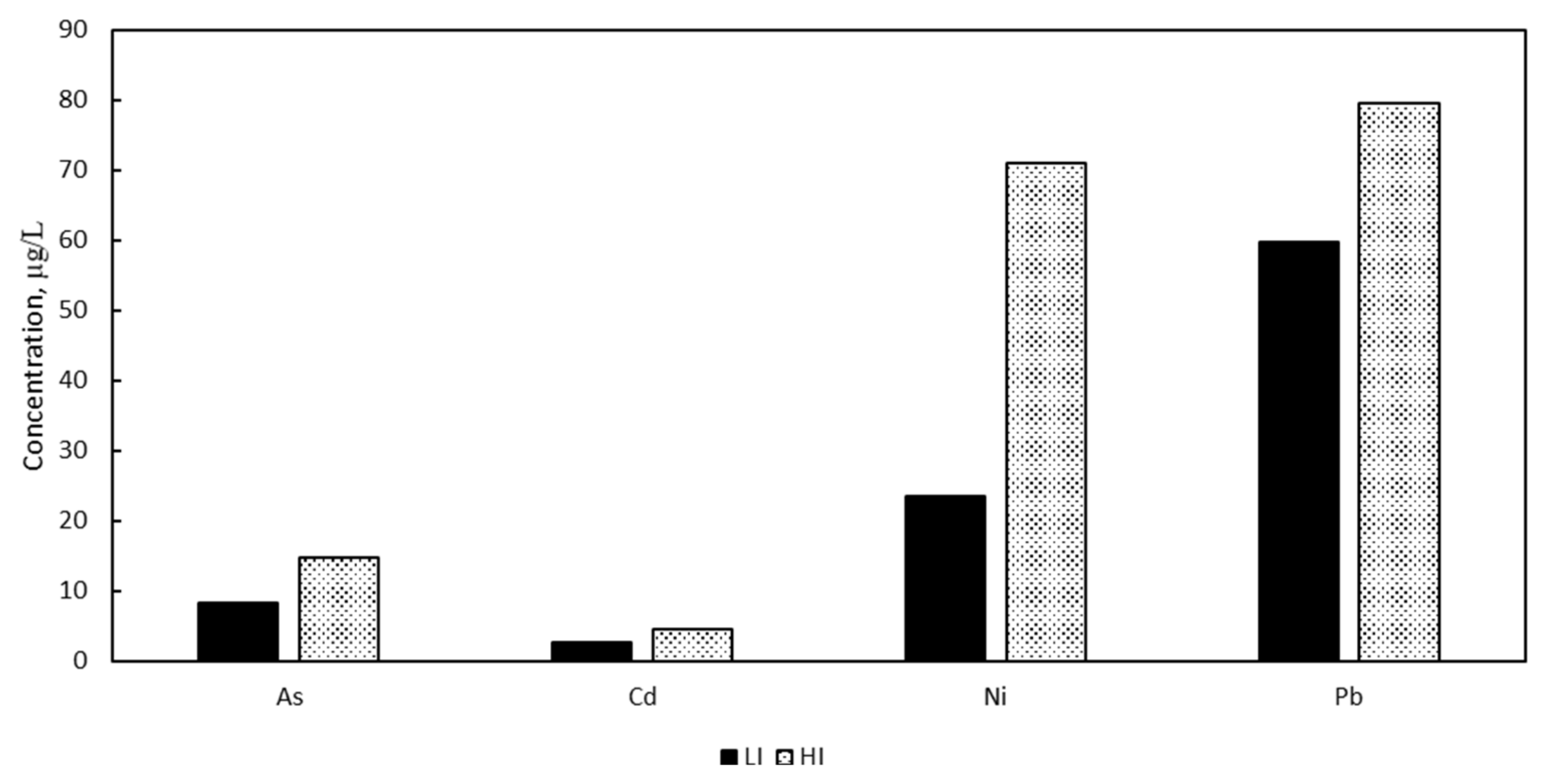
| Arsenic | 8 | 15 | 6–12 | 9–23 |
| Cadmiums | 2.6 | 4.5 | 1.4–5.1 | 2.1–9.4 |
| Nickel | 23.5 | 71 | 8–68.4 | 26.1–193 |
| Lead | 59.7 | 79.6 | 39.3–90.7 | 46.6–135.9 |
| 2016 | Station | ||||
|---|---|---|---|---|---|
| HI Area | LI Area | ||||
| AS | AC | AI | OL | ||
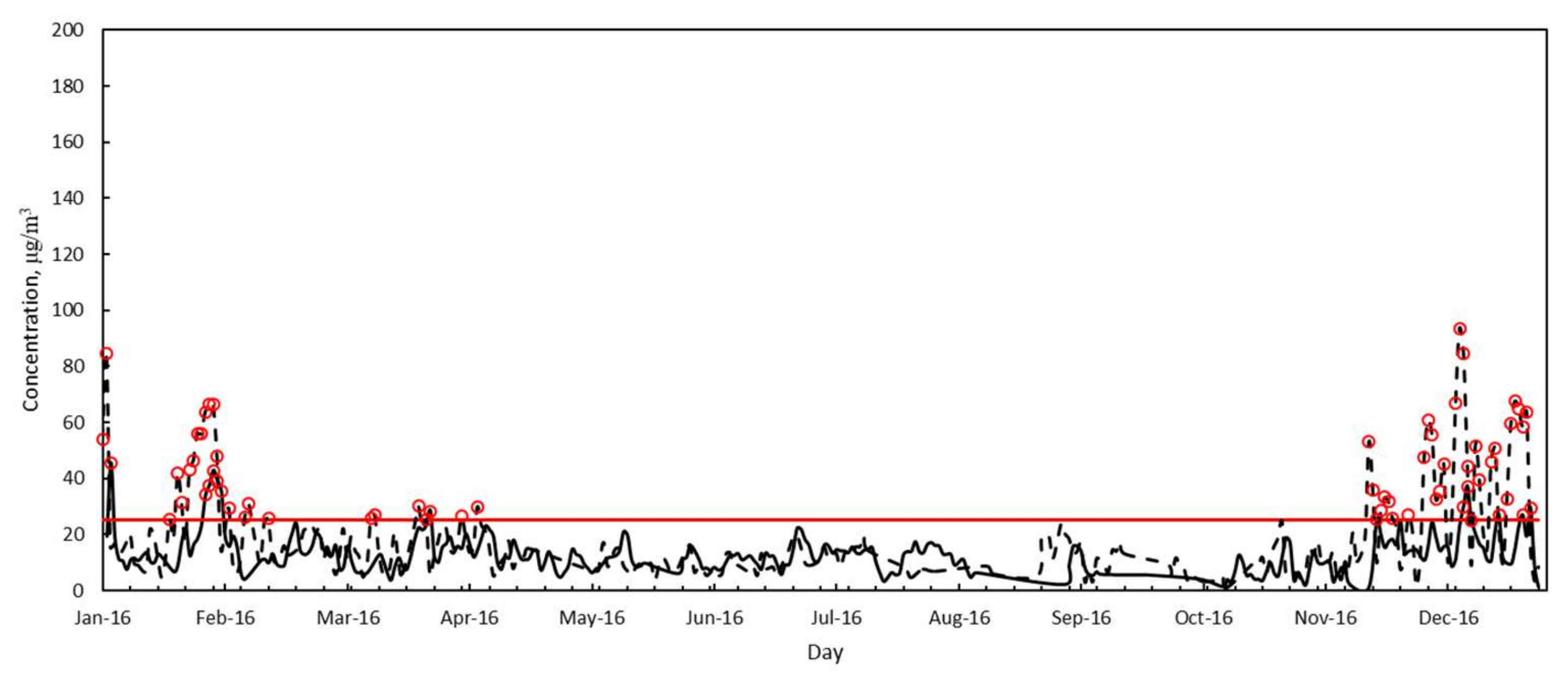
| PM10 | Annual average, μg/m3 | 39.4 | 42.5 | 33.6 | 25.7 |
| Standard deviation, μg/m3 | 26.6 | 24.1 | 20.6 | 13.6 | |
| Minimum, μg/m3 | 1.8 | 5 | 2.8 | 3.2 | |
| Maximum, μg/m3 | 159.2 | 150.3 | 139.6 | 83.5 | |
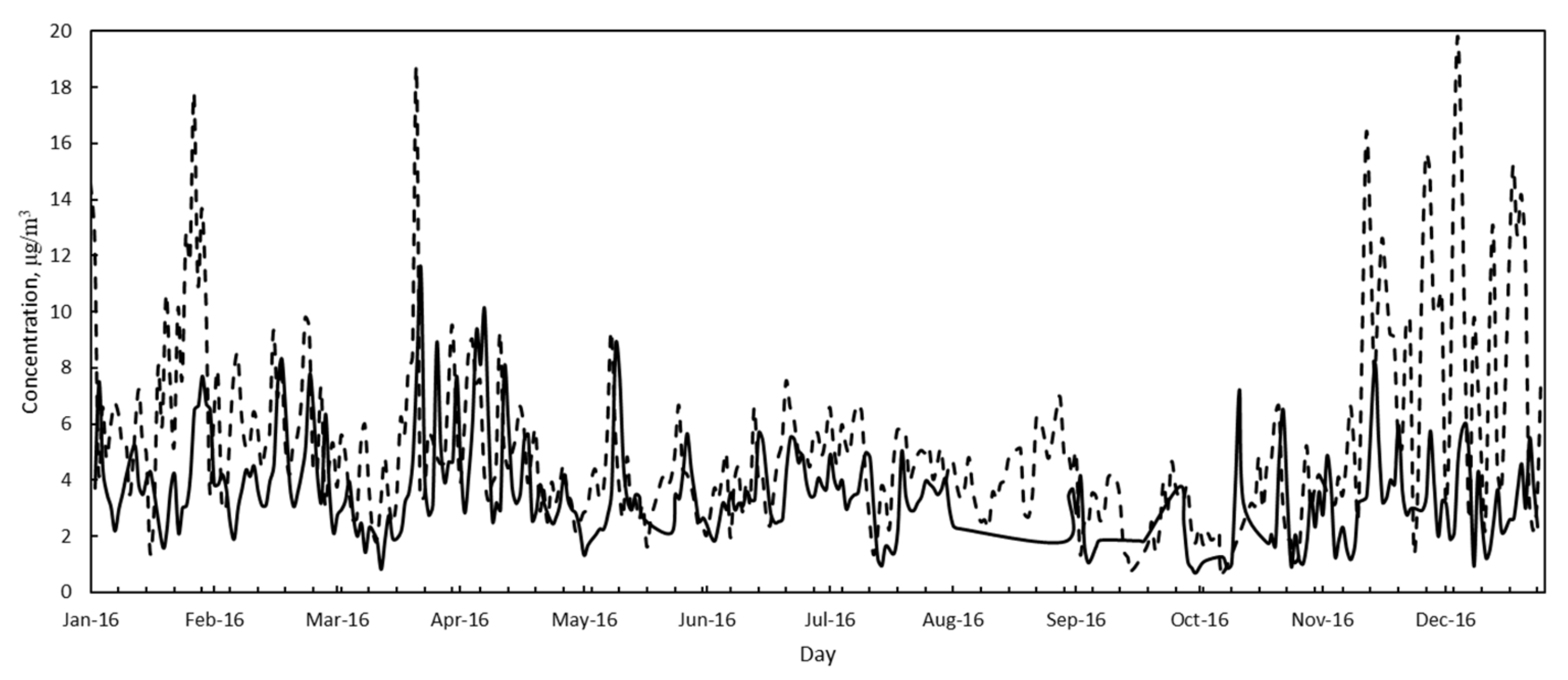
| PM2.5 | Annual average, μg/m3 | 18.0 | --- | 17.8 | 18.8 |
| Standard deviation, μg/m3 | 25.2 | --- | 18.7 | 10.5 | |
| Minimum, μg/m3 | 1.8 | --- | 0.4 | 0.9 | |
| Maximum, μg/m3 | 104.5 | --- | 84.5 | 45.5 | |
| HI Area | LI Area | ||
|---|---|---|---|
| As | Annual average/± StandDev, μg/m3 | 0.6 ± 0.4 | 0.4 ± 0.2 |
| % in PM10 | 1.7 | 1.5 | |
| Cd | Annual average/± StandDev, μg/m3 | 0.5 ± 0.3 | 0.3 ± 0.2 |
| % in PM10 | 14 | 13 | |
| Ni | Annual average/± StandDev, μg/m3 | 5.1 ± 3.2 | 3.0 ± 2.1 |
| % in PM10 | 14 | 12 | |
| Pb | Annual average/± StandDev, μg/m3 | 0.08 ± 0.00 | 0.1 ± 0.003 |
| % in PM10 | 0.25 | 0.25 |
| Arsenic (As) | Cadmium (Cd) | Nickel (Ni) | Lead (Pb) | |||||
|---|---|---|---|---|---|---|---|---|
| LI Area | HI Area | LI Area | HI Area | LI Area | HI Area | LI Area | HI Area | |
| January | 1.58 | 3.24 | 1.30 | 2.67 | 13.02 | 26.70 | 0.02 | 0.05 |
| February | 1.77 | 2.43 | 1.46 | 2.01 | 14.61 | 20.05 | 0.03 | 0.04 |
| March | 1.48 | 2.15 | 1.22 | 1.77 | 12.18 | 17.67 | 0.02 | 0.03 |
| April | 1.89 | 2.19 | 1.56 | 1.81 | 15.56 | 18.06 | 0.03 | 0.03 |
| May | 1.19 | 1.66 | 0.98 | 1.37 | 9.80 | 13.65 | 0.02 | 0.02 |
| June | 1.45 | 1.70 | 1.19 | 1.40 | 11.91 | 14.00 | 0.02 | 0.03 |
| July | 1.41 | 2.04 | 1.16 | 1.68 | 11.64 | 16.83 | 0.02 | 0.03 |
| August | 0.26 | 1.80 | 0.21 | 1.49 | 2.15 | 14.85 | 0.00 | 0.03 |
| September | 0.36 | 1.20 | 0.29 | 0.99 | 2.94 | 9.86 | 0.01 | 0.02 |
| October | 0.74 | 1.00 | 0.61 | 0.82 | 6.07 | 8.23 | 0.01 | 0.01 |
| November | 1.20 | 2.59 | 0.99 | 2.13 | 9.89 | 21.32 | 0.02 | 0.04 |
| December | 1.33 | 3.97 | 1.10 | 3.27 | 10.98 | 32.69 | 0.02 | 0.06 |
Publisher’s Note: MDPI stays neutral with regard to jurisdictional claims in published maps and institutional affiliations. |
© 2022 by the authors. Licensee MDPI, Basel, Switzerland. This article is an open access article distributed under the terms and conditions of the Creative Commons Attribution (CC BY) license (https://creativecommons.org/licenses/by/4.0/).
Share and Cite
Lotrecchiano, N.; Montano, L.; Bonapace, I.M.; Giancarlo, T.; Trucillo, P.; Sofia, D. Comparison Process of Blood Heavy Metals Absorption Linked to Measured Air Quality Data in Areas with High and Low Environmental Impact. Processes 2022, 10, 1409. https://doi.org/10.3390/pr10071409
Lotrecchiano N, Montano L, Bonapace IM, Giancarlo T, Trucillo P, Sofia D. Comparison Process of Blood Heavy Metals Absorption Linked to Measured Air Quality Data in Areas with High and Low Environmental Impact. Processes. 2022; 10(7):1409. https://doi.org/10.3390/pr10071409
Chicago/Turabian StyleLotrecchiano, Nicoletta, Luigi Montano, Ian Marc Bonapace, Tenore Giancarlo, Paolo Trucillo, and Daniele Sofia. 2022. "Comparison Process of Blood Heavy Metals Absorption Linked to Measured Air Quality Data in Areas with High and Low Environmental Impact" Processes 10, no. 7: 1409. https://doi.org/10.3390/pr10071409
APA StyleLotrecchiano, N., Montano, L., Bonapace, I. M., Giancarlo, T., Trucillo, P., & Sofia, D. (2022). Comparison Process of Blood Heavy Metals Absorption Linked to Measured Air Quality Data in Areas with High and Low Environmental Impact. Processes, 10(7), 1409. https://doi.org/10.3390/pr10071409