
A Homotopy Method for the Constrained Inverse Problem in the Multiphase Porous Media Flow

 ,
, 

Abstract
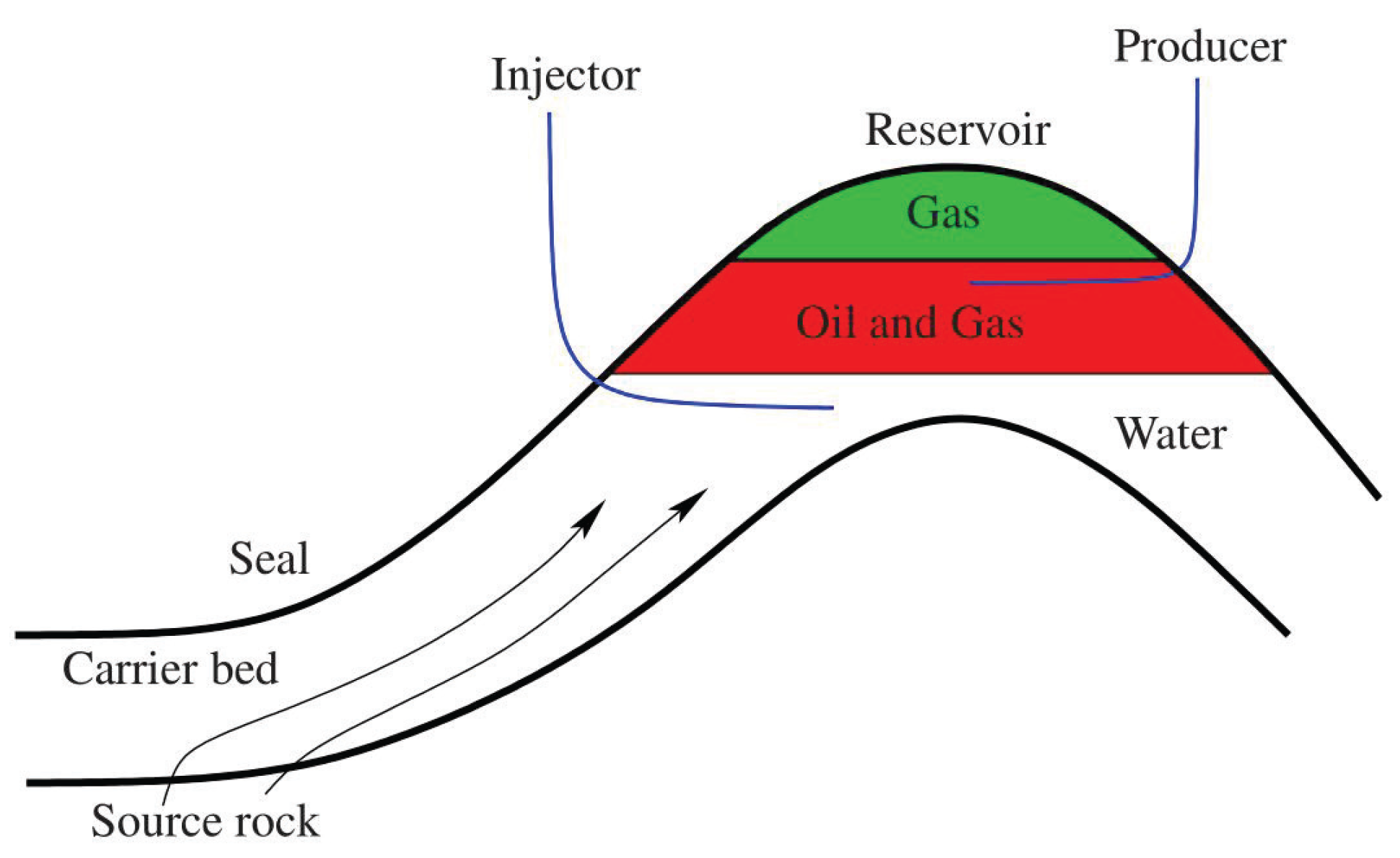
1. Introduction
2. Discretization
3. Identification Method
3.1. Basic Iterative Method
3.2. Homotopy Method
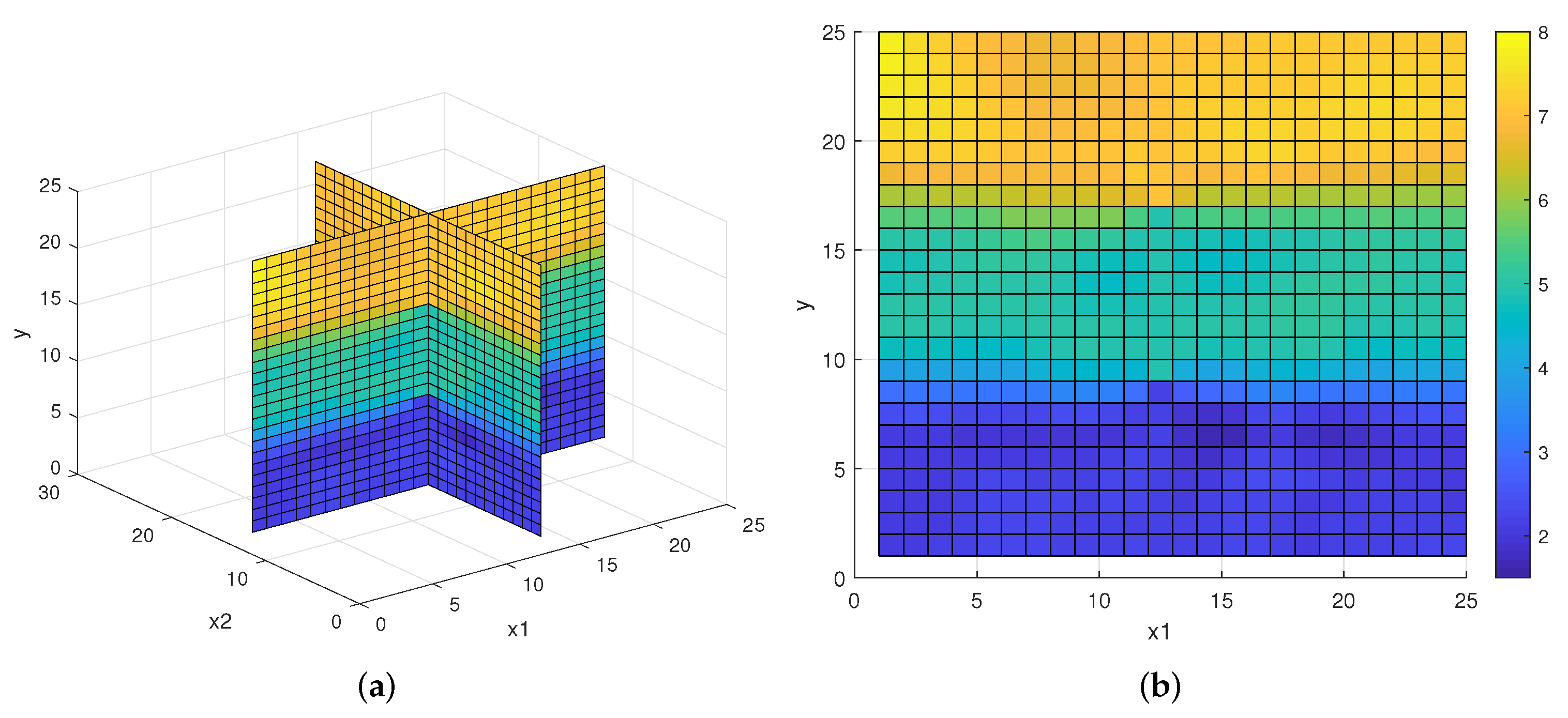
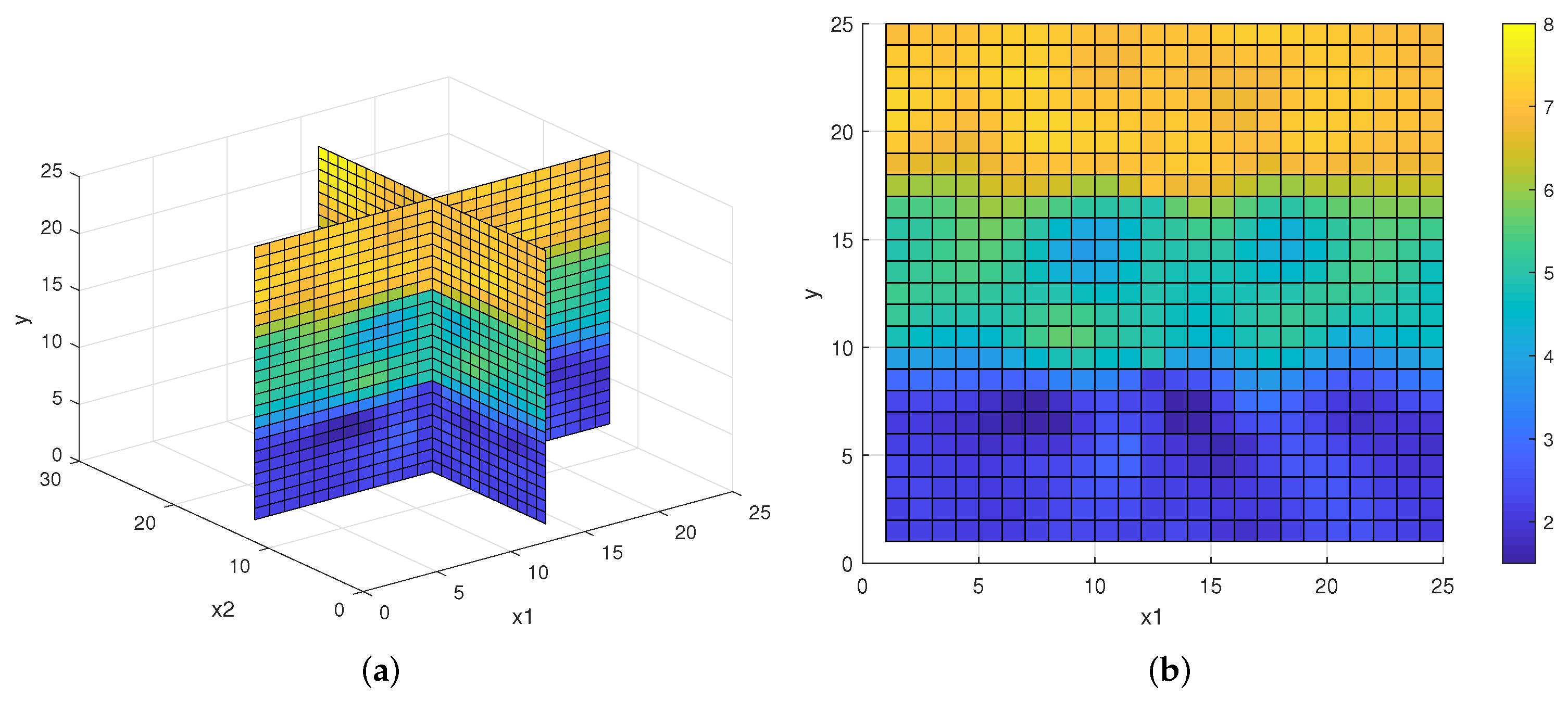
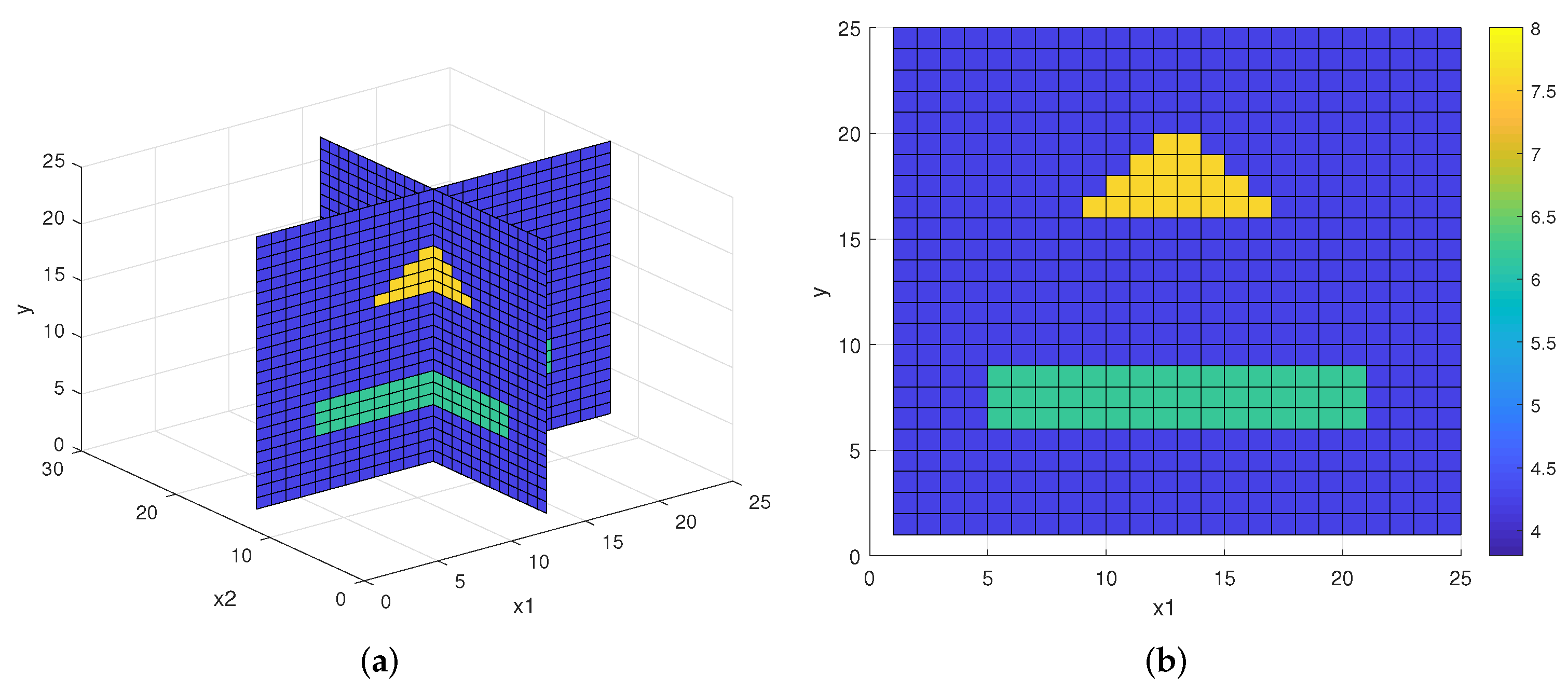
4. Numerical Experiments
- (1)
- The stability of the homotopy method with constraints is better than the homotopy method without constraints;
- (2)
- The region of convergence of the homotopy strategy is wider than the basic iterative method with constraints;
- (3)
- The homotopy method with constraints has wide convergence region and strong anti-noise ability.
5. Conclusions
Author Contributions
Funding
Institutional Review Board Statement
Informed Consent Statement
Data Availability Statement
Acknowledgments
Conflicts of Interest
Appendix A. Discretization of the Diffusion Term
Appendix B. Discretization of the Convection Term
Appendix B.1. Buckley–Leverett Flux Function
Appendix B.2. Buckley–Leverett Flux Function with Gravitational Effects
References
- Rana, B.M.J.; Arifuzzaman, S.M.; Islam, S.; Reza-E-Rabbi, S.; Al-Mamun, A.; Mazumder, M.; Roy, K.C.; Khan, M.S. Swimming of microbes in blood flow of nano-bioconvective Williamson fluid. Therm. Sci. Eng. Progr. 2021, 25, 101018. [Google Scholar] [CrossRef]
- Reza-E-Rabbi, S.; Ahmmed, S.F.; Arifuzzaman, S.M.; Sarkar, T.; Khan, M.S. Computational modelling of multiphase fluid flow behaviour over a stretching sheet in the presence of nanoparticles. Eng. Sci. Technol. Int. J. 2020, 23, 605–617. [Google Scholar] [CrossRef]
- Moosavian, N. Pipe network modeling for analysis of flow in porous media. Can. J. Civil Eng. 2019, 46, 1151–1159. [Google Scholar] [CrossRef]
- Shapiro, A.A. Mechanics of the separating surface for a two-phase co-current flow in a porous medium. Transp. Porous Med. 2016, 112, 489–517. [Google Scholar] [CrossRef]
- Hunt, A.G.; Sahimi, M. Flow, transport, and reaction in porous media: Percolation scaling, critical-path analysis, and effective medium approximation. Rev. Geoph. 2017, 55, 993–1078. [Google Scholar] [CrossRef]
- Espedal, M.S.; Karlsen, K.H. Numerical solution of reservoir flow models based on large time step operator splitting algorithm. In Filtration in Porous Media and Industrial Applications: Lecture Notes in Mathematics; Fasano, A., Ed.; Springer: Berlin/Heidelberg, Germany, 2000; Volume 1734, pp. 9–77. [Google Scholar]
- Saeed, S.T.; Riaz, M.B.; Baleanu, D.; Akgul, A.; Husnine, S.M. Exact analysis of second grade fluid with generalized boundary conditions. Intell. Autom. Soft Comput. 2021, 28, 547–559. [Google Scholar] [CrossRef]
- Saeed, S.T.; Abro, K.A.; Almani, S. Role of single slip assumption on the viscoelastic liquid subject to non-integer differentiable operators. Math. Meth. Appl. Sci. 2021, 44, 6005–6020. [Google Scholar] [CrossRef]
- Saeed, S.T.; Riaz, M.B.; Baleanu, D.; Abro, K.A. A mathematical study of natural convection flow through a channel with non-singular kernels: An application to transport phenomena. Alex. Eng. J. 2020, 59, 2269–2281. [Google Scholar] [CrossRef]
- Abdeljawad, T.; Riaz, M.B.; Saeed, S.T.; Iftikhar, N.I. MHD Maxwell fluid with heat transfer analysis under ramp velocity and ramp temperature subject to non-integer differentiable operators. Comput. Model. Eng. Sci. 2021, 126, 821–841. [Google Scholar] [CrossRef]
- Firdous, H.; Saeed, S.T.; Ahmad, H.; Askar, S. Using non-Fourier’s heat flux and non-Fick’s mass flux theory in the radiative and chemically reactive flow of Powell-Eyring fluid. Energies 2021, 14, 6882. [Google Scholar] [CrossRef]
- Riaz, M.B.; Siddique, I.; Saeed, S.T.; Atangana, A. MHD Oldroyd-B fluid with slip condition in view of local and nonlocal kernels. J. Appl. Comput. Mech. 2021, 7, 116–127. [Google Scholar]
- Riaz, M.B.; Saeed, S.T. Comprehensive analysis of integer order, Caputo-Fabrizio and Atangana-Baleanu fractional time derivative for MHD Oldroyd-B fluid with slip effect and time dependent bounday conditions. Discr. Contin. Dynam. Syst. 2021, 14, 3719–3746. [Google Scholar] [CrossRef]
- Hazra, S.; Class, H.; Helmig, R.; Schulz, V. Forward and inverse problems in modeling of multiphase flow and transport through porous media. Computat. Geosci. 2004, 8, 21–47. [Google Scholar] [CrossRef]
- Wang, J.; Zabaras, N. A Markov random field model of contamination source identification in porous media flow. Int. J. Heat Mass Transf. 2006, 49, 939–950. [Google Scholar] [CrossRef]
- Nilssen, T.K.; Karlsen, K.H.; Mannseth, T.; Tai, X.C. Identification of diffusion parameters in a nonlinear convection-diffusion equation using the augmented lagrangian method. Comput. Geosci. 2009, 13, 317–329. [Google Scholar] [CrossRef][Green Version]
- Yan, B.; Harp, D.R.; Chen, B.; Pawar, R. A physics-constrained deep learning model for simulating multiphase flow in 3D heterogeneous porous media. Fuel 2022, 313, 122693. [Google Scholar] [CrossRef]
- Yan, B.; Chen, B.; Harp, D.R.; Jia, W.; Pawar, R.J. A robust deep learning workflow to predict multiphase flow behavior during geological CO2 sequestration injection and Post-Injection periods. J. Hydrol. 2022, 607, 127542. [Google Scholar] [CrossRef]
- Magzymov, D.; Ratnakar, R.R.; Dindoruk, B.; Johns, R.T. Evaluation of machine learning methodologies using simple physics based conceptual models for flow in porous media. In Proceedings of the SPE Annual Technical Conference and Exhibition, Dubai, United Arab Emirates, 21–23 September 2021. [Google Scholar]
- Almajid, M.M.; Abu-Al-Saud, M.O. Prediction of porous media fluid flow using physics informed neural networks. J. Petrol. Sci. Eng. 2022, 208, 109205. [Google Scholar] [CrossRef]
- Jackson, D.D. Interpretation of inaccurate, insufficient and inconsistent data. Geophys. J. R. Astron. Soc. 1972, 28, 97–109. [Google Scholar] [CrossRef]
- Watson, L.T. Globally convergent homotopy methods: A tutorial. Appl. Math. Comput. 1989, 31, 369–396. [Google Scholar]
- Mousa, M.M.; Alsharari, F. Convergence and error estimation of a new formulation of homotopy perturbation method for classes of nonlinear integral/integro-differential equations. Mathematics 2021, 9, 2244. [Google Scholar] [CrossRef]
- Agarwal, P.; Akbar, M.; Nawaz, R.; Jleli, M. Solutions of system of Volterra integro-differential equations using optimal homotopy asymptotic method. Math. Meth. Appl. Sci. 2021, 44, 2671–2681. [Google Scholar] [CrossRef]
- Mousa, M.M.; Kaltayev, A. Homotopy perturbation method for solving nonlinear differential-difference equations. Z. Naturforsch. A 2010, 65, 511–517. [Google Scholar] [CrossRef]
- Hammad, H.A.; Agarwal, P.; Guirao, J.L.G. Applications to boundary value problems and homotopy theory via tripled fixed point techniques in partially metric spaces. Mathematics 2021, 9, 2012. [Google Scholar] [CrossRef]
- Mousa, M.M.; Kaltayev, A. Application of the homotopy perturbation method to a magneto-elastico-viscous fluid along a semi-infinite plate. Int. J. Nonlinear Sci. Numer. Simul. 2009, 10, 1113–1120. [Google Scholar] [CrossRef]
- Saad, K.M.; Iyiola, O.S.; Agarwal, P. An effective homotopy analysis method to solve the cubic isothermal auto-catalytic chemical system. AIMS Math. 2018, 3, 183–194. [Google Scholar] [CrossRef]
- Mallick, A.; Ranjan, R.; Das, R. Application of homotopy perturbation method and inverse prediction of thermal parameters for an annular fin subjected to thermal load. J. Therm. Stress. 2016, 39, 298–313. [Google Scholar] [CrossRef]
- Mallick, A.; Ranjan, R.; Prasad, D.K.; Das, R. Inverse prediction and application of homotopy perturbation method for efficient design of an annular fin with variable thermal conductivity and heat generation. Math. Model. Anal. 2016, 21, 699–717. [Google Scholar] [CrossRef]
- Biswal, U.; Chakraverty, S.; Ojha, B.K. Application of homotopy perturbation method in inverse analysis of Jeffery-Hamel flow problem. Eur. J. Mech. B Fluid. 2021, 86, 107–112. [Google Scholar] [CrossRef]
- Sattari Shajari, P.; Shidfar, A. Application of weighted homotopy analysis method to solve an inverse source problem for wave equation. Inverse Probl. Sci. Eng. 2019, 27, 61–88. [Google Scholar] [CrossRef]
- Liu, T. A multigrid-homotopy method for nonlinear inverse problems. Comput. Math. Appl. 2020, 79, 1706–1717. [Google Scholar] [CrossRef]
- Liu, T. A wavelet multiscale-homotopy method for the parameter identification problem of partial differential equations. Comput. Math. Appl. 2016, 71, 1519–1523. [Google Scholar] [CrossRef]
- Hu, L.; Huang, L.; Lu, Z.R. Crack identification of beam structures using homotopy continuation algorithm. Inverse Probl. Sci. Eng. 2017, 25, 169–187. [Google Scholar] [CrossRef]
- Courbot, J.B.; Colicchio, B. A fast homotopy algorithm for gridless sparse recovery. Inverse Probl. 2021, 37, 025002. [Google Scholar] [CrossRef]
- Słota, D.; Chmielowska, A.; Brociek, R.; Szczygieł, M. Application of the homotopy method for fractional inverse Stefan problem. Energies 2020, 13, 5474. [Google Scholar] [CrossRef]
- Liu, J.; Wang, B. Solving the backward heat conduction problem by homotopy analysis method. Appl. Numer. Math. 2018, 128, 84–97. [Google Scholar] [CrossRef]
- Liu, T. Porosity reconstruction based on Biot elastic model of porous media by homotopy perturbation method. Chaos Soliton. Fract. 2022, 158, 112007. [Google Scholar] [CrossRef]
- Enting, I.G.; Pearman, G.I. Description of a one-dimensional carbon cycle model calibrated using techniques of constrained inversion. Tellus B 1987, 39, 459–476. [Google Scholar] [CrossRef][Green Version]
- Lambert, M.; Lesselier, D. Binary-constrained inversion of a buried cylindrical obstacle from complete and phaseless magnetic fields. Inverse Probl. 2000, 16, 563–576. [Google Scholar] [CrossRef]
- Atzberger, C.; Richter, K. Spatially constrained inversion of radiative transfer models for improved LAI mapping from future Sentinel-2 imagery. Remote Sens. Environ. 2012, 120, 208–218. [Google Scholar] [CrossRef]
- Auken, E.; Christiansen, A.V. Layered and laterally constrained 2D inversion of resistivity data. Geophysics 2004, 69, 752–761. [Google Scholar] [CrossRef]
- Zhao, J.; Liu, T.; Liu, S. An adaptive homotopy method for permeability estimation of a nonlinear diffusion equation. Inverse Probl. Sci. Eng. 2013, 21, 585–604. [Google Scholar] [CrossRef]
- Liu, T. Parameter estimation with the multigrid-homotopy method for a nonlinear diffusion equation. J. Comput. Appl. Math. 2022, 413, 114393. [Google Scholar] [CrossRef]
- Engquist, B.; Osher, S. One-sided difference approximations for nonlinear conservation laws. Math. Comp. 1981, 36, 321–351. [Google Scholar] [CrossRef]


| Parameter | Definition |
|---|---|
| absolute permeability | |
| total Darcy velocity | |
| total mobility of phases | |
| p | global pressure |
| density of wetting phase | |
| h | height |
| porosity | |
| injection well | |
| production well | |
| mobility ratio | |
| relative permeability | |
| viscosity | |
| density | |
| phase mobility of nonwetting phase |
| Example Number | Noise Level | HMC | HM | BIMC |
|---|---|---|---|---|
| 4.1 | 5% | 6.22% | 6.90% | × |
| 10% | 6.38% | 7.40% | × | |
| 15% | 7.13% | × | × | |
| 20% | 7.44% | × | × | |
| 4.2 | 5% | 5.71% | 6.47% | × |
| 10% | 5.81% | 7.39% | × | |
| 15% | 6.06% | × | × | |
| 20% | 7.19% | × | × |
Publisher’s Note: MDPI stays neutral with regard to jurisdictional claims in published maps and institutional affiliations. |
© 2022 by the authors. Licensee MDPI, Basel, Switzerland. This article is an open access article distributed under the terms and conditions of the Creative Commons Attribution (CC BY) license (https://creativecommons.org/licenses/by/4.0/).
Share and Cite
Liu, T.; Xia, K.; Zheng, Y.; Yang, Y.; Qiu, R.; Qi, Y.; Liu, C. A Homotopy Method for the Constrained Inverse Problem in the Multiphase Porous Media Flow. Processes 2022, 10, 1143. https://doi.org/10.3390/pr10061143
Liu T, Xia K, Zheng Y, Yang Y, Qiu R, Qi Y, Liu C. A Homotopy Method for the Constrained Inverse Problem in the Multiphase Porous Media Flow. Processes. 2022; 10(6):1143. https://doi.org/10.3390/pr10061143
Chicago/Turabian StyleLiu, Tao, Kaiwen Xia, Yuanjin Zheng, Yanxiong Yang, Ruofeng Qiu, Yunfei Qi, and Chao Liu. 2022. "A Homotopy Method for the Constrained Inverse Problem in the Multiphase Porous Media Flow" Processes 10, no. 6: 1143. https://doi.org/10.3390/pr10061143
APA StyleLiu, T., Xia, K., Zheng, Y., Yang, Y., Qiu, R., Qi, Y., & Liu, C. (2022). A Homotopy Method for the Constrained Inverse Problem in the Multiphase Porous Media Flow. Processes, 10(6), 1143. https://doi.org/10.3390/pr10061143