Forecasting Oil Production Flowrate Based on an Improved Backpropagation High-Order Neural Network with Empirical Mode Decomposition

Abstract

Developing a forecasting model for oilfield well production plays a significant role in managing mature oilfields as it can help to identify production loss earlier. It is very common that mature fields need more frequent production measurements to detect declining production. This study proposes a machine learning system based on a hybrid empirical mode decomposition backpropagation higher-order neural network (EMD-BP-HONN) for oilfields with less frequent measurement. With the individual well characteristic of stationary and non-stationary data, it creates a unique challenge. By utilizing historical well production measurement as a time series feature and then decomposing it using empirical mode decomposition, it generates a simpler pattern to be learned by the model. In this paper, various algorithms were deployed as a benchmark, and the proposed method was eventually completed to forecast well production. With proper feature engineering, it shows that the proposed method can be a potentially effective method to improve forecasting obtained by the traditional method.

1. Introduction

One important activity in the oil industry is to measure well production. By conducting measurements of the oil production, it could show how the well performs compared to the simulation result. Moreover, it plays a significant role in the phase of declining production. By measuring the declining production earlier, petroleum engineers have the capability to deliver appropriate action to respond [1,2]. However, such an ideal situation of providing continuous and periodic measurements is not viable to deploy due to economic and technical challenges [3,4]. Non-continuous and occasional basis of well production measurement is very common in oilfield operation [5,6].

Commonly, well production rate is measured using a test separator for some minutes to hours and then applying certain calculations to represent the whole day production of the well. In more advanced technology, the rate is measured by multiphase flow meters (MPFMs) that are equipped with several sensors, such as an ultrasonic meter that is used for gas rate measurement and a capacitance meter that can measure very high water cut, which is barely possible to acquire using the conventional method [7,8]. In many oil fields, a production test is not acquired every day for each well due to the well number limitation of test stations to conduct the test. Therefore, conducting specific tasks such as well performance monitoring will rely on a lagged test that leads to late action when something occurs in the well. Hence, petroleum engineers have difficulty determining declining well production earlier. For a longer production span, some traditional approaches are common to forecast production, including decline curve analysis (DCA), exploration interpolation and the black oil model [9]. Since those forecasting models need to be tuned with proper parameters and pick the right slope, its main disadvantage is a subjective judgment by the expert who is conducting the analysis [3]. For shorter-term prediction, many approaches have been proposed using data-driven methodology, such as using thermogravimetric data to predict oil flow rate [4], inferring flow rate from real-time parameters using diverse neural networks [10] and many data mining methodologies. Another study involves additional hardware such as extended venturi and the use of a support vector machine (SVM) for the model [11]. Another experiment was augmented by a lab-scale vertical pipe to obtain differential pressure signals as the inputs to principal component analysis and neural network models [12].

In the well production forecasting area, the use of artificial intelligence and data mining method have been introduced in the last two decades. The research literature is basically divided into two approaches: non-time series (cross-sectional data) and time series, either univariate or multivariate approaches. 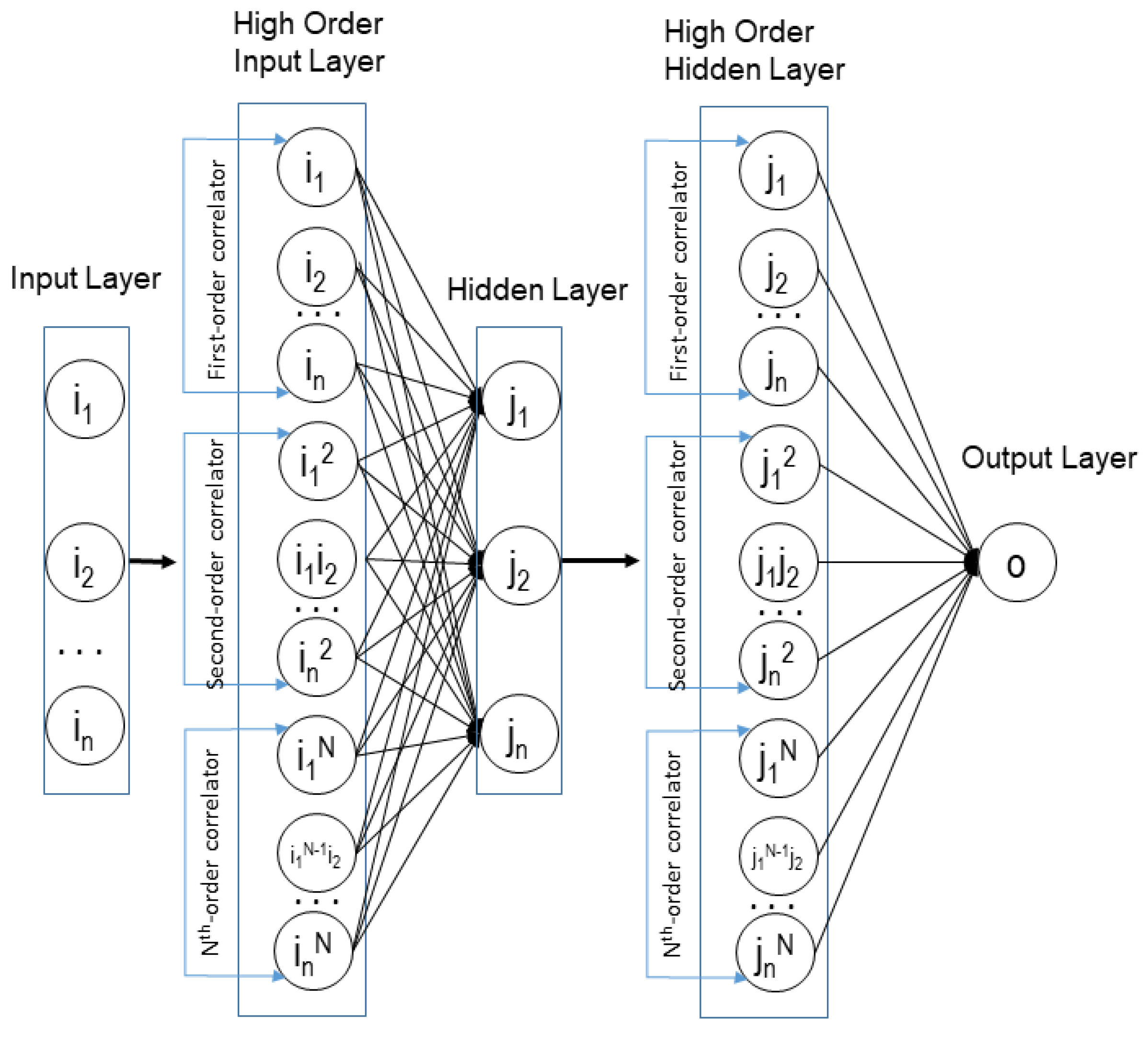Some efforts were intended to improve the prediction by exploiting optimization algorithms such as the imperialist competitive algorithm [13] and aquila optimizer [14]. To capture highly non-linear correlation, the higher-order neural network (HONN) has been introduced to forecast cumulative oil production [15]. A more recent experiment utilized a univariate and multivariate time series approach using a nonlinear autoregressive neural network with exogenous input (NARX) to forecast oil production in a natural fracture reservoir [16]. Another approach with a multi-layer multi-valued neural network (MLMVN) was developed for predicting oil production [17]. This model is based on complex numbers for the input and weight parameters of neural network nodes. The advantage of MLMVN is a derivative-free learning approach which benefits from requiring fewer resources and a faster process [18]. Another approach uses an ensemble neural network with adaptive simulated annealing to optimize the combining strategy [10]. Dongyan et al. [19] proposed ensemble univariate algorithms, namely autoregressive integrated moving average (ARIMA) and long short-term memory (LSTM). The most recent one is the approach using deep long-short term memory (DLSTM) as an extension to the traditional recurrent neural network [20]; however, this research only focuses on non-stationary time series well production data. An interesting approach was performed by decomposing the production data before inputting it into the model [21].

Even though the univariate forecasting method is very popular in other topics, such as crude oil price forecasting [22] and electrical load forecasting [23], only a few studies focused on the univariate time series prediction of oil flow rate. In a previous study, the multivariate model in certain cases showed better results than the univariate one [16]; however, multivariate has its own limitation, such as requiring more dependent variables to be collected. All of the literature confirms that oil production is non-linear and needs a special approach to capture such complex behavior [24]. One of the complex behaviors came from the disturbance factor of oil flow rate measurement noise. According to previous literature, noise reduction is a contributing factor to achieving an excellent univariate forecasting method [15]. Another gap in previous univariate time series forecasting for oil production is the focus on non-stationary data [20], which may not cover all the characteristics of well production.

In this study, we propose a novel hybrid model for time series well production forecasting data using a back propagation higher-order neural network (BP-HONN) with first, second and third-order synaptic operation and the decomposition method. The decomposition method utilizes simplifying the trend of input data (signal); thus, the neural network could learn it more accurately. Based on a recent study, as the effect of decomposition, increasing the linearity of time series data could improve accuracy performance [9]. For the decomposition, empirical mode decomposition (EMD) is being proposed, as it is proven for a non-linear dataset in other research areas [24,25]. To evaluate the robustness of the model, the stationary and non-stationary time series data are being used. The actual field dataset was taken from previous literature [15] and production data from the Sumatra Basin field, Indonesia, a total of 30 wells of production data. In addition, another novel hybrid model is also being introduced as the benchmark. The same dataset will be evaluated with EMD-BP-MLMVN to show the performance comparison of the proposed model.

The contributions of this research are:

• The introduction of a novel hybrid method incorporating EMD and BP-HONN as the main proposed framework for forecasting short term oil production.
• The introduction of a secondary novel hybrid framework utilizing EMD and BP-MLMVN for the same objective.
• Providing a 25-well dataset from an actual oilfield consisting of stationary and non-stationary datasets, which is a real representation of business challenges. This dataset will be available for future work by other researchers.
• The experiment shows that the proposed method EMD-BP-HONN are significantly better than other benchmark models.

The remainder of this paper explains the oilfield/reservoir description where the dataset is retrieved, the algorithms that are used, the selected performance evaluation and eventually, the framework proposed. The final result will be discussed in the result section alongside the statistical test to evaluate the significant difference among models.

2. Materials and Methods

2.1. The Reservoir under Study

The experiment data are carried out from two sources. The first one is from previous literature [18], which provides real production data from 5 (five) wells in Cambay Basin (CB), India. The top depth of the reservoir is between 1380–1413 m, with initial reservoir pressure observed at around 144 kg/cm³. The reservoir reserved oil in place was estimated at around 2.47 MMt. This oilfield started production in February 2000 with CB1 (first well). In September 2009, the cumulative oil produced for the CB1 well was 0.156 MMt. Other wells were drilled in subsequent years. Each well has 63 data points which were taken for each month from the year 2004 to 2009.

The descriptive statistics of those datasets are listed in

Table 1. Descriptive statistic of Cambay Basin dataset.

Well	Count	Min	Mean	Max	Std Dev	Skew	Kurtosis	ADF Statistic 1
CB1	63	28.5	494.4	1054.5	223.5	0.86	0.36	−1.929
CB2	63	161.5	546.9	1786.0	470.2	1.55	1.10	−1.820
CB3	63	2650.5	4094.5	5928.0	1091.2	0.24	−1.59	−1.870
CB4	63	247.0	531.2	950.0	182.0	0.36	−0.86	−0.942
CB5	63	161.5	1016.0	2251.5	633.0	0.41	−1.15	−0.866

¹ Critical value (5%) at −2.92.

. In addition to common statistic measurement, to test the stationarity of the data, the augmented Dickey–Fuller (ADF) test was used as per [26,27]. The null hypothesis of stationarity is rejected whenever the ADF statistic value is above critical values. Hence, all CB well’s production data are categorized as non-stationer.

The second source of experiment data comes from an actual oilfield in the Central Sumatra Basin (CS), Indonesia. The field was discovered in 1952, and it has been producing since 1971. The field area is around 19,905 acres, and currently, it is produced by 220 oil producer wells in either single or commingles production. The reservoir consists of multiple productive sands with depths between 4200–4400 ft and thicknesses around 0.13–158 ft. Regarding rock properties, the sand has permeability between 10 to 1200 mD and porosity around 10–34%. The oil is considered a light oil type with a value of gravity of 0.8°. In this experiment, 25 (twenty-five) wells were selected that consist of stationary and non-stationary characteristics to evaluate the model prediction robustness. Descriptive statistics of those datasets are listed in

Table 2. Descriptive statistic of Central Sumatra Basin dataset.

Well	Count	Min	Mean	Max	Std Dev	Skew	Kurtosis	ADF Statistic 1	Hurst
CS1	113	722.7	1515.8	4111.3	764.2	2.18	4.62	2.49	0.63
CS2	192	774.4	4778.1	5861.4	1317.3	−1.41	1.55	2.38	0.50
CS3	215	849.6	1988.3	6249.6	1407.8	1.63	1.76	2.18	0.68
CS4	143	737.8	2907.3	4440.2	692.1	−1.00	3.32	2.10	0.69
CS5	215	13397	13887	14718	305.7	0.98	−0.01	1.44	0.51
CS6	151	839.2	3120.5	6851.2	1525.6	1.27	1.02	−3.49	0.45
CS7	106	450.8	590.8	693.6	49.5	−0.64	0.41	−3.52	0.44
CS8	215	169.5	523.5	1042.8	199.0	0.37	−0.54	−2.28	0.31
CS9	212	1974.5	7294.8	8745.4	1879.4	−1.96	2.45	−3.60	0.63
CS10	121	1470.6	5817.7	7646.2	1949.2	−1.03	−0.09	−3.60	0.80
CS11	112	2.35	649.0	1392.0	362.1	−0.20	−1.22	−2.10	0.30
CS12	117	288.0	949.6	1822.2	310.2	−0.04	−0.43	−2.14	0.37
CS13	115	255.0	1968.4	3304.0	670.3	−0.27	−0.25	−2.08	0.43
CS14	106	510.0	1401.2	2028.0	450.4	−0.46	−1.34	−1.04	0.57
CS15	112	1332.0	1991.5	2508.0	229.0	−0.10	−0.39	−2.03	0.38
CS16	115	36.0	311.5	660.0	147.8	0.12	−1.00	−1.36	0.25
CS17	116	2.8	192.4	464.0	83.5	0.51	0.54	−3.74	0.21
CS18	114	180.0	575.3	890.4	155.7	−0.45	−0.05	−1.85	0.36
CS19	117	330.0	1215.9	1864.8	470.4	−0.33	−1.25	−1.44	0.46
CS20	107	558.0	1614.0	1215.8	283.2	−0.69	−0.77	−1.76	0.52
CS21	111	2535.7	2727.2	3044.6	118.4	0.47	−0.55	−1.75	0.28
CS22	108	668.0	1037.6	1444.9	190.4	−0.19	−1.31	−1.08	0.57
CS23	112	872.4	1298.2	1557.8	171.5	−0.89	−0.17	−3.59	0.39
CS24	117	753.0	3523.0	5616.0	904.5	0.15	−0.67	−0.82	0.60
CS25	103	672.0	1074.9	1567.7	198.0	−0.19	−0.65	−1.71	0.52

¹ Critical value (5%) at −2.89.

. Those well datasets with higher ADF statistics belong to the non-stationary category. Another statistical characteristic being measured is the Hurst exponent value, indicating volatility, roughness and smoothness time-series data [16]. The completed dataset is provided in Supplementary Material.

2.2. Higher-Order Neural Networks (HONN)

Most artificial neural networks (ANN) use linear neurons, where the linear connection exists between the input vector and synaptic-weight vector Naturally, the correlation between input and neuron weight is considered non-linear. To overcome this, one neural network variance was introduced [18]. The major difference between HONN and conventional ANN is how the weighted sum of the input vector is calculated. The operation of synaptic weight and input is defined as:

$$\begin{array}{cc}v=w_0{x}_0+{\displaystyle {\displaystyle \sum }_{i_1=1}^n}& w_{i_1}{x}_{i_1}+{\displaystyle {\displaystyle \sum }_{i_1=1}^n}{\displaystyle {\displaystyle \sum }_{i_2=i_1}^n}{w}_{i_1{i}_2}{x}_{i_1}{x}_{i_2}\\ & +\cdots {\displaystyle {\displaystyle \sum }_{i_1=1}^n}{\displaystyle {\displaystyle \sum }_{i_2=i_1}^n}\cdots {\displaystyle {\displaystyle \sum }_{i_N=i_{N-1}}^n}{w}_{i_1{i}_2}{\cdots }_{i_N}{x}_{i_1}{x}_{i_2}\cdots x_{i_N}\end{array}$$

(1)

where $x_{\mathrm{i}}$ is the neuron input of ith element of X, $w_{\mathrm{i}}$ is the weight of neuron input of ith, $x_0$ is the bias neuron input, $w_0$ is the weight of bias and $v$ is the output of the synaptic operation. Additionally, the somatic operation to calculate the outputs is described as

$$y=\phi \left(v\right)$$

(2)

where y is the output of the neural network and $\phi$ is the activation function. Architecture-wise, as illustrated in Figure 1, HONN have interconnected layers, and the input vector will be calculated in each correlator (order) and then applied to the weighted sum of those.

Suppose we have a neural network structure, as shown in Figure 1.

First, we must carry out a feed-forward operation by the initial weight, and the input then calculates the error.

$$Error=\frac{1}{2}{\left(output-O_{out}\right)}^2$$

(3)

where output is the desired output and $O_{out}$ is the neural output (or y). We begin backpropagating the error from the output layer to the hidden layer.

$$\frac{dError}{d{W}_{jo}}=\frac{dError}{d{O}_{out}}\times \frac{d{O}_{out}}{d{O}_{in}}\times \frac{d{O}_{in}}{d{W}_{jo}}$$

(4)

Recall the error formula to calculate the derivative error.

$$\frac{dError}{d{O}_{out}}=-\left(output-O_{out}\right)$$

(5)

The derivative output layer node-out to output layer node-in is derivative of its activation function

$$\frac{d{O}_{out}}{d{O}_{in}}={\phi }^{\prime }\left(O_{in}\right)$$

(6)

Output layer node-in is calculated by multiplying the weight and input of the high order hidden layer node.

$$\frac{d{O}_{in}}{d{W}_{jo}}=J_{ho}$$

(7)

Then, we continue backpropagating the error from the hidden layer to the input layer.

$$\frac{dError}{d{W}_{ij}}=\frac{dError}{d{J}_{out}}\times \frac{d{J}_{out}}{d{J}_{in}}\times \frac{d{J}_{in}}{d{W}_{ij}}$$

(8)

Derivative error to hidden layer:

$$\frac{dError}{d{J}_{out}}=\frac{dError}{d{O}_{in}}\times \frac{d{O}_{in}}{d{J}_{out}}=\left(\frac{dError}{d{O}_{out}}\times \frac{d{O}_{out}}{d{O}_{in}}\right)\times \frac{d{O}_{in}}{d{J}_{out}}$$

(9)

We already calculated $\frac{dError}{d{O}_{out}}$ and $\frac{d{O}_{out}}{d{O}_{in}}$ in the previous step. To calculate $\frac{d{O}_{in}}{dJout},$ recall the high order synaptics operation when we conducted the feed-forward.

$$O_{in}=J_1{w}_{J_{1}O}+J_2{w}_{J_{2}O}+J_1^2{w}_{J_{11}O}+J_1{J}_2{w}_{J{12}_o}+J_2^2{w}_{J{22}_o}+..$$

(10)

Thus,

$$\frac{d{O}_{in}}{d{J}_{1_{out}}}=w_{J_{1}O}+0+2J_1{w}_{J_{11}O}+J_1{w}_{J{12}_o}+0+..$$

(11)

$$\frac{d{O}_{in}}{d{J}_{2_{out}}}=0+w_{J_{2}O}+0+J_2{w}_{J{12}_o}+2J_2{w}_{J{22}_o}+..$$

(12)

The derivative hidden layer node-out to hidden layer node in is derivative of its activation function

$$\frac{d{J}_{out}}{d{J}_{in}}={\varnothing }^{\prime }\left(J_{in}\right)$$

(13)

Hidden layer node-in is calculated by multiplying the weight and input of the high order input layer node.

$$\frac{d{J}_{in}}{d{W}_{ij}}=I_{ho}$$

(14)

The error (squared error) is minimized by updating the weight matrix as

$$W_{k+1}=W_k+\mathsf{\Delta }{W}_k$$

(15)

where the change in weight matric is denoted by $\mathsf{\Delta }{W}_k$ which is proportional to the gradient of the error function as

$$\mathsf{\Delta }{W}_k=-\eta \frac{dErro{r}_k}{d{W}_k}$$

(16)

where η > 0 is the learning rate which affects the performance of the algorithm during the updating process.

2.3. Multi-Layer Neural Network with Multi-Valued Neurons (MLMVN)

MLMVN is a multi-layer neural network consisting of Multi-Valued Neurons (MVN) as basic neurons with complex-valued weights, which becomes the key difference between MLMVN and the classic neural network. The difference makes the learning process in MLMVN simpler and means that it has a better capability of generalization.

All neurons in the network are complex numbers located on the unit circle and the weights. An input/output mapping of a continuous MVN is described by a function of n variables

$$f\left(x_1,\dots ,x_n\right)=P\left(w_0+w_1{x}_1+\cdots +w_n{x}_n\right), f:O^n\to O$$

(17)

where $O$ is a set of points located on the unit circle, $x_{\mathrm{i}}$ is the neuron input of ith element of X, $w_{\mathrm{i}}$ is the weight of neuron input of ith element of X, $x_0$ is the bias neuron input, $w_0$ is the weight of bias.

The continuous MVN activation function (as in Figure 2) is

$$P\left(z\right)=e^{iArg\left(z\right)}=\frac{z}{\left|z\right|}$$

(18)

where $z=w_0+w_1{x}_1+\cdots +w_n{x}_n$ is the weighted sum, $Arg\left(z\right)$ is the main value of the argument of the complex number z. Thus, a continuous MVN output is a projection of its complex-valued weighted sum onto the unit circle.

The MVN training is based on the error-correction learning rule (Figure 3) as follows:

$$W_{r+1}=W_r+\frac{C_r}{\left(n+1\right)\left|z_r\right|}\left(D-Y\right)\overline{X}$$

(19)

where $\overline{X}$ is the array of neuron inputs complex-conjugated, $n$ is the number of neuron inputs, $D$ is the expected target of the neuron, $Y=P\left(z\right)$ is the calculated output of the neuron, $r$ is the number of the epoch step, $W_r$ is the current weighting vector, $W_{r+1}$ is the new weighting vector, $C_r$ is a learning rate and $\left|z_r\right|$ is the current absolute value of the weighted sum.

The MLMVN learning algorithm is derivative-free. It is based on the same error-correction learning rule as the one of a single MVN. Let MLMVN contain $m$ layers of neurons and $x_1,\dots ,x_n$ be the network inputs. To obtain the local errors for all neurons, the global error of

$${\delta }_{jm}^{*}=D_{jm}-Y_{jm}$$

(20)

must be shared with these neurons. Therefore, the errors of the $m$th (output) layer neurons are

$${\delta }_{jm}=\frac{1}{t_m}{\delta }_{jm}^{*}$$

(21)

where $j_m$specifies the $j$th neuron of the $m$th layer; $t_m=N_m+1$. The errors of the hidden layer’s neurons are

$${\delta }_{js}=\frac{1}{t_s}{{\displaystyle \sum }}_{j=1}^{N_s+1}{\delta }_{js+1}{\left(w_i^{js+1}\right)}^{-1}$$

(22)

where $j_s$ specifies the $j$th neuron of the $s$th layer; $t_s=N_{s-1}+1$, $s=2,\dots ,m$ is the number of all neurons in the layer $s-1$, and $t_1=n+1$ ($n$ is the number of network inputs).

After the error backpropagation is completed, the weights for all connecting layers shall then be updated using the error-correction learning rule adapted to MLMVN. It means that while it is used for the hidden neurons, the factor $\frac{1}{\left|z_r\right|}$ should not be applied to the output neurons thus it becomes $W_{r+1}=W_r+\frac{C_r}{\left(n+1\right)}\left(D-Y\right)\overline{X}$ in this output layer.

2.4. Empirical Mode Decomposition (EMD)

Empirical mode decomposition (EMD), also known as the Hilbert–Huang transformation (HHT), is a method to decompose signals into several simpler signals, called intrinsic mode functions (IMF) [28]. This method is an empirical approach to obtain current frequency data from a dataset, which preferably has non-stationer and non-linear characteristics [29,30]. Each IMF has to satisfy only one extrema that crosses the zero line (zero-crossing), with a mean value of zero. Due to its nature, the number of IMF obtained cannot be pre-determined; thus, every dataset has its own number of IMF and residue (last monotonic functions). The final result of EMD with the aggregation of all its components (and residue) can be seen as

$$x\left(t\right)={{\displaystyle \sum }}_{i=1}^n\left(c_i\right)+r_n$$

(23)

where $x\left(t\right)$ is the time-series signal, is the ith IMF and $r_n$ is the residue.

2.5. Performance Evaluation

In this research, several performance metrics are used, such as R² (coefficient of determination), root mean square error (RMSE) and mean absolute percentage error (MAPE), as follows:

$$R^2=1-\frac{{{\displaystyle \sum }}_{i=0}^{n-1}{\left(y_i-{\widehat{y}}_i\right)}^2}{{{\displaystyle \sum }}_{i=0}^{n-1}{\left(y_i-\overline{y}\right)}^2}$$

(24)

$$RMSE=\sqrt{\frac{1}{n}{{\displaystyle \sum }}_{i=0}^{n-1}{\left(y_i-{\widehat{y}}_i\right)}^2}$$

(25)

$$MAPE=\frac{100\%}{n}{{\displaystyle \sum }}_{i=0}^{n-1}\left|\frac{y_i-{\widehat{y}}_i}{y_i}\right|$$

(26)

where $y_i$is the actual target for $i_{th}$component, ${\widehat{y}}_i$ is the predicted value, $\overline{y}$ is the mean value and n is the amount data.

2.6. Framework of the Proposed Model

In this research, a hybrid model of combining EMD and HONN with a backpropagation learning method is proposed to forecast the oil flow rate of 30 well production data. Another hybrid model of EMD and MLMVN is also introduced as a benchmark. The proposed method includes several steps, as shown in Figure 4. The first step is to deliver pre-processing of all datasets. The pre-processing started by normalizing all values to the same range. For the CB dataset, the scaler was applied as in the original paper, which calculated the ratio to maximum production (9500 m³) [15]. For the CS dataset, a min-max scaler (−1 to 1) is applied for HONN and 0 to 1 for MLMVN. Additionally, the normalized value is processed with an EMD algorithm which constructs multiple IMFs (and residue) for each dataset. Due to the fact that the proposed learning algorithms are not able to learn from time-series data directly, the feature transformation using a lag feature transforms to the supervised-learning dataset. For this research, two up to five prior time series data were selected as inputs (i.e., X_t−5, X_t−4, X_t−3, X_t−2, X_t−1, for the lag feature of five) and the subsequent time series as a target (y). Then, the transformed feature feeds into HONN with the backpropagation learning method. For HONN and EMD-HONN, we chose hyperparameter as follows: the network architecture is one hidden layer for the activation function of tanh-tanh, the initial learning rate is 0.001 and is adaptive to the error of each epoch; if the error decreases, the learning rate multiplies by 0.7 and 1.05 if the error increase. The iteration for backpropagation learning (epoch) is 600, and the momentum is 0.9. The experiment was repeated with different hidden neuron configurations from 2 to 10 and also with the polynomial synaptic operation of linear (LSO), quadratic (QSO) and cubical (CSO). The best-performed model was selected to compete with other benchmark models.

For the second hybrid model introduced using EMD-MLMVN, a similar framework has been utilized, with BP-HONN being replaced with BP-MLMVN. The architecture of BP-MLMVN of 1 hidden layer, with randomized initial weight and number of training epochs of 500. The experiment was repeated with different hidden neurons configuration from 2 to 10 to select the best performing configuration.

Additionally, three other forecasting methods were utilized for benchmarking. The most basic forecasting method is persistence or naïve, which takes the previous value (X_t−1) as the next step value (X_t+1) or forecasted value. For a more advanced baseline, two time series forecasting algorithms are used: autoregressive integrated moving average (ARIMA) and long short-term memory (LSTM). ARIMA is a very popular statistical model for forecasting time series data. It consists of three components: autoregression (p), moving average (q) and differencing (d). For this experiment, the variable p, d, q values are selected from 1 to 4. LSTM as the variance of recurrent neural network (RNN) can capture nonlinearity trends of well production forecast [19]. The hyperparameters for LSTM are the number of layers and activation function. The best of 20, 50 and 200 layers with combinations of tanh, relu and sigmoid activation functions are selected as the benchmarks for the proposed model.

3. Results and Discussion

3.1. Result of CB and CS Datasets

The result of the proposed methods and other benchmark methods for both oilfields are presented in this section. As mentioned in the previous section, the proposed models repeated runs with different parameters and configurations and selected the best to compete with benchmark models. An example of the best configuration for several wells can be seen in

Table 3. Best result of HONN-based methods on several wells.

Well	Methods	No. of Hidden Neurons	Synaptic Operation	Lag	MAPE	R2	RMSE
CB1	BP-HONN	2	CSO	5	34.77	0.87	0.004
	EMD-BP-HONN	3	CSO	3	33.86	0.90	0.003
CS2	BP-HONN	6	CSO	4	5.76	0.97	214.15
	EMD-BP-HONN	9	CSO	2	5.16	0.99	118.49
CS18	BP-HONN	3	CSO	2	4.07	0.14	74.62
	EMD-BP-HONN	6	CSO	3	2.09	0.81	34.69

, which shows that different lag features and the number of hidden neurons provide the best MAPE. In the summary, as seen in

Table 4. Result of CB oilfield in MAPE metric. The lowest score is in bold.

Well	Persistence	ARIMA	LSTM	BP-HONN	BP-MLMVN	EMD-BP-HONN	EMD-BP-MLMVN
CB1	58.8217	51.1220	85.6711	34.7721	49.5745	33.8551	24.6530
CB2	8.1251	3.2276	7.5459	3.6933	4.2213	3.6687	3.0037
CB3	5.9905	5.1662	6.8647	2.7992	9.2329	1.7264	4.4384
CB4	8.8297	7.7091	7.5996	5.9757	6.5168	2.2271	2.6348
CB5	22.0980	22.5708	26.8748	22.1773	24.6941	20.2176	24.6921

,

Table 5. Result of CB oilfield in RMSE metric. The lowest score is in bold.

Well	Persistence	ARIMA	LSTM	BP-HONN	BP-MLMVN	EMD-BP-HONN	EMD-BP-MLMVN
CB1	0.00551	0.00480	0.00676	0.00361	0.00695	0.00318	0.00276
CB2	0.01336	0.00674	0.01408	0.00807	0.00818	0.00689	0.00674
CB3	0.02946	0.02520	0.03293	0.01407	0.04957	0.00956	0.02327
CB4	0.00333	0.00285	0.00248	0.00290	0.00263	0.00091	0.00095
CB5	0.04342	0.04616	0.04532	0.03075	0.05439	0.02217	0.01977

,

Table 6. Result of CB oilfield in R² metric. The highest score is in bold.

Well	Persistence	ARIMA	LSTM	BP-HONN	BP-MLMVN	EMD-BP-HONN	EMD-BP-MLMVN
CB1	0.70758	0.778648	0.832072	0.874414	0.535006	0.902602	0.926822
CB2	0.533407	0.881093	0.746193	0.82976	0.825121	0.87584	0.881261
CB3	0.897148	0.92478	0.854823	0.976548	0.708902	0.989175	0.935841
CB4	0.729598	0.80199	0.476615	0.795313	0.831711	0.979662	0.978109
CB5	0.341114	0.255405	0.389998	0.669492	0.016875	0.828181	0.863412

and

Table 7. Result of CS oilfield in MAPE metric. The lowest score is in bold.

Well	Persistence	ARIMA	LSTM	BP-HONN	BP-MLMVN	EMD-BP-HONN	EMD-BP-MLMVN
CS1	3.6933	2.9200	3.5937	4.4857	5.8110	3.8575	5.7848
CS2	7.0161	5.9889	9.4525	5.7664	27.0809	5.1646	7.6287
CS3	2.2222	2.0381	3.5247	3.3583	3.7679	3.0959	3.6221
CS4	1.0469	0.7155	0.9131	1.0340	1.1026	1.0184	0.5969
CS5	0.2214	0.1850	0.2117	0.1940	0.4261	0.1295	0.0957
CS6	0.8595	0.7304	0.7838	0.7078	0.7072	0.7061	0.6763
CS7	1.0125	0.9918	1.0067	0.8609	10.2040	0.7166	8.2757
CS8	16.8791	12.3467	12.9215	11.5983	15.8302	8.9814	10.3197
CS9	0.2833	0.1979	0.2027	0.2371	0.4662	0.2130	0.3398
CS10	0.6888	0.6293	0.5143	0.4623	0.5642	0.4420	0.3449
CS11	350.2999	377.4806	409.8470	88.3414	99.2139	51.6295	47.3973
CS12	10.1758	9.9895	10.7328	19.3471	25.0963	15.2705	20.9661
CS13	8.8332	9.8213	12.3169	6.1035	7.4236	3.8197	5.7077
CS14	7.2523	5.8126	5.8123	3.0850	2.9582	2.4229	1.8676
CS15	5.0698	4.5538	5.3236	5.6101	6.8687	4.4302	5.7963
CS16	42.9258	46.7672	75.0410	1.7973	1.5646	0.5894	0.7129
CS17	68.4740	72.0464	90.0719	1.8375	1.9177	1.6845	1.1904
CS18	7.0018	6.7551	10.4111	4.0748	3.9908	2.0935	2.6025
CS19	6.0988	6.4009	7.0253	10.7183	11.9264	8.5481	9.4610
CS20	5.9032	5.7425	5.2782	5.2151	5.2374	2.6710	2.3559
CS21	2.2704	1.8905	2.3375	4.5688	4.8310	2.8859	3.2109
CS22	4.0042	3.4350	3.2347	3.7852	3.7051	2.3720	2.4807
CS23	5.1769	4.5989	4.2936	15.6620	20.6448	14.9554	20.2448
CS24	6.1914	7.3289	11.5756	2.8008	3.2835	2.3956	1.9994
CS25	4.7480	4.9989	3.6993	3.9649	4.0291	2.1641	2.0224

, the proposed EMD-BP-HONN and EMD-MLMVN outperformed all benchmarked models with the smallest MAPE in 23 out of 30 wells. Interestingly, ARIMA models have a decent result compared to our proposed models. For other metrics measured, RMSE and R2 have consistent results, as seen in Table 5 and Table 6 for the CB dataset, in which the proposed methods have better forecasting performance than the benchmark models. Additionally, for detailed prediction, as an example, the prediction result of the proposed models for CB2 are presented in Figure 5 and Figure 6. The prediction results of the proposed models for CS18 are presented in Figure 7 and Figure 8.

Another interesting finding, based on the result, is that the hybrid model indeed improves the performance of the base model. As seen in Table 4 and Table 7, by implementing EMD in the pre-processing stage, both BP-HONN and BP-MLMVN have been improved, on average, by 23% and 34%, respectively.

In regard to comparing our work to other studies, other studies proposed a DLSTM model that outperforms the HONN vanilla model for the Cambay Basin dataset [20]. However, instead of individual well production, the dataset used is the cumulative production of five wells, as in Table 1. Based on the result, the reported MAPE scores are 2.851 and 3.459 for DLSTM and vanilla-HONN, respectively. To compare the performance of EMD-BP-HONN and EMD-BP-MLMVN, the same dataset was carried out, and the result can be seen in

Table 8. Comparison to other study for cumulative production of Cambay Basin Oilfield.

Metric	DLSTM 1	Vanilla-HONN 1	LSTM	BP-HONN	BP-MLMVN	EMD-BP-HONN	EMD-BP-MLMVN
MAPE	2.851	3.459	4.04	2.86	2.19	1.28	1.39
RMSE	0.025	0.035	0.037	0.031	0.019	0.010	0.013
R2	-	-	0.6	0.8	0.92	0.98	0.97

¹ Reprinted/adapted with permission from Ref. [20]. Copyright 2022, copyright Elsevier, License Number: 5320830137007.

. EMD-BP-HONN continues to show better performance than other methods that are reported in other papers.

3.2. Statistical Tests

In this section, a statistical test was applied to evaluate whether there is a significant difference between the methods being proposed and the benchmark models. The Friedman test uses null and alternative hypotheses. The null hypothesis (H0) implies that the mean for each population is equal; thus, there is no significant difference among methods. The alternate hypothesis implies that at least one population mean is different from the rest. If the p-value of the test is less than 0.05, the null hypothesis can be rejected.

Using the Friedman chi-square test (using scipy python library) with MAPE metrics for all datasets, the results are as follows: statistic = 52.828 and p-value = 1.270 × 10⁻⁹. Seeing this result, the null hypothesis can be rejected. Then, to determine which methods are significantly different, the Nemenyi post hoc test was utilized, and the result is shown in Figure 9. The result shows that EMD-BP-HONN is significantly different from other benchmark methods except with EMD-BP-MLMVN. EMD-BP-MLMVN significantly differs from persistence and LSTM; however, it is not significantly different from ARIMA and BP-HONN.

4. Conclusions

In this study, we introduced a hybrid model of EMD-BP-HONN and EMD-BP-MLMVN for oil flow rate forecasting. The decomposition method of EMD was utilized in the pre-processing stage to make time-series data simpler; thus, it should increase the performance of the forecasting algorithm. The proposed methods were applied to 30 datasets collected from two oilfields, Cambay Basin, India and the Central Sumatra Basin, Indonesia. To compare the performance, time-series forecasting was tested as well. The proposed methods have significant results and outperformed the benchmark models in most datasets. In addition, by implementing the decomposition method prior to base models, the hybrid models were improved significantly in all datasets.

For future works, the hybrid models being proposed, EMD-BP-HONN and EMD-BP-MLMVN, could be improved with a more advanced version of the decomposition method. Selecting the best parameter can also be explored using an optimization algorithm to be able to search global optimum of parameters.

References

1. Meribout, M.; Al-Rawahi, N.; Al-Naamany, A.; Al-Bemani, A.; Al-Busaidi, K.; Meribout, A. Integration of impedance measurements with acoustic measurements for accurate two phase flow metering in case of high water-cut. Flow Meas. Instrum. 2010, 21, 8–19. [Google Scholar] [CrossRef]
2. Höök, M.; Davidsson, S.; Johansson, S.; Tang, X. Decline and depletion rates of oil production: A comprehensive investigation. Philos. Trans. R. Soc. London. Ser. A Math. Phys. Eng. Sci. 2014, 372, 20120448. [Google Scholar] [CrossRef] [PubMed]
3. Huang, Z.; Xie, D.; Zhang, H.; Li, H. Gas–oil two-phase flow measurement using an electrical capacitance tomography system and a Venturi meter. Flow Meas. Instrum. 2005, 16, 177–182. [Google Scholar] [CrossRef]
4. Pourabdollah, K.; Mokhtari, B. Flow rate measurement of individual oil well using multivariate thermal analysis. Measurement 2011, 44, 2028–2034. [Google Scholar] [CrossRef]
5. Ganat, T.A.; Hrairi, M.; Hawlader, M.; Farj, O. Development of a novel method to estimate fluid flow rate in oil wells using electrical submersible pump. J. Pet. Sci. Eng. 2015, 135, 466–475. [Google Scholar] [CrossRef]
6. Henry, M.; Tombs, M.; Zhou, F. Field experience of well testing using multiphase Coriolis metering. Flow Meas. Instrum. 2016, 52, 121–136. [Google Scholar] [CrossRef]
7. Thorn, R.; Johansen, G.A.; Hjertaker, B.T. Three-phase flow measurement in the petroleum industry. Meas. Sci. Technol. 2013, 24, 012003. [Google Scholar] [CrossRef]
8. Geoffrey, F.H.; Alimonti, C. Multiphase flow metering. In Developments in Petroleum Science; Elsevier: Amsterdam, The Netherlands, 2009; p. 329. [Google Scholar]
9. Wang, M.; Fan, Z.; Xing, G.; Zhao, W.; Song, H.; Su, P. Rate Decline Analysis for Modeling Volume Fractured Well Production in Naturally Fractured Reservoirs. Energies 2018, 11, 43. [Google Scholar] [CrossRef] [Green Version]
10. Al-Qutami, T.A.; Ibrahim, R.; Ismail, I.; Ishak, M.A. Virtual multiphase flow metering using diverse neural network ensemble and adaptive simulated annealing. Expert Syst. Appl. 2018, 93, 72–85. [Google Scholar] [CrossRef]
11. Xu, L.; Zhou, W.; Li, X.; Tang, S. Wet Gas Metering Using a Revised Venturi Meter and Soft-Computing Approximation Techniques. IEEE Trans. Instrum. Meas. 2011, 60, 947–956. [Google Scholar] [CrossRef]
12. Shaban, H.; Tavoularis, S. Measurement of gas and liquid flow rates in two-phase pipe flows by the application of machine learning techniques to differential pressure signals. Int. J. Multiph. Flow 2014, 67, 106–117. [Google Scholar] [CrossRef]
13. Ahmadi, M.A.; Ebadi, M.; Shokrollahi, A.; Majidi, S.M.J. Evolving artificial neural network and imperialist competitive algorithm for prediction oil flow rate of the reservoir. Appl. Soft Comput. 2013, 13, 1085–1098. [Google Scholar] [CrossRef]
14. AlRassas, A.M.; Al-Qaness, M.A.A.; Ewees, A.A.; Ren, S.; Elaziz, M.A.; Damaševičius, R.; Krilavičius, T. Optimized ANFIS Model Using Aquila Optimizer for Oil Production Forecasting. Processes 2021, 9, 1194. [Google Scholar] [CrossRef]
15. Chakra, N.C.; Song, K.-Y.; Gupta, M.M.; Saraf, D.N. An innovative neural forecast of cumulative oil production from a petroleum reservoir employing higher-order neural networks (HONNs). J. Pet. Sci. Eng. 2013, 106, 18–33. [Google Scholar] [CrossRef]
16. Sheremetov, L.; Cosultchi, A.; Martínez-Muñoz, J.; Gonzalez-Sánchez, A.; Jiménez-Aquino, M. Data-driven forecasting of naturally fractured reservoirs based on nonlinear autoregressive neural networks with exogenous input. J. Pet. Sci. Eng. 2014, 123, 106–119. [Google Scholar] [CrossRef]
17. Aizenberg, I.; Sheremetov, L.; Villa-Vargas, L.; Martinez-Muñoz, J. Multilayer Neural Network with Multi-Valued Neurons in time series forecasting of oil production. Neurocomputing 2016, 175, 980–989. [Google Scholar] [CrossRef]
18. Aizenberg, I.; Moraga, C. Multilayer Feedforward Neural Network Based on Multi-valued Neurons (MLMVN) and a Backpropagation Learning Algorithm. Soft Comput. 2007, 11, 169–183. [Google Scholar] [CrossRef]
19. Fan, D.; Sun, H.; Yao, J.; Zhang, K.; Yan, X.; Sun, Z. Well production forecasting based on ARIMA-LSTM model considering manual operations. Energy 2021, 220, 119708. [Google Scholar] [CrossRef]
20. Sagheer, A.; Kotb, M. Time series forecasting of petroleum production using deep LSTM recurrent networks. Neurocomputing 2019, 323, 203–213. [Google Scholar] [CrossRef]
21. Liu, W.; Gu, J. Forecasting oil production using ensemble empirical model decomposition based Long Short-Term Memory neural network. J. Pet. Sci. Eng. 2020, 189, 107013. [Google Scholar] [CrossRef]
22. Wu, J.; Miu, F.; Li, T. Daily Crude Oil Price Forecasting Based on Improved CEEMDAN, SCA, and RVFL: A Case Study in WTI Oil Market. Energies 2020, 13, 1852. [Google Scholar] [CrossRef] [Green Version]
23. Fan, G.-F.; Peng, L.-L.; Hong, W.-C.; Sun, F. Electric load forecasting by the SVR model with differential empirical mode decomposition and auto regression. Neurocomputing 2016, 173, 958–970. [Google Scholar] [CrossRef]
24. Jin, F.; Li, Y.; Sun, S.; Li, H. Forecasting air passenger demand with a new hybrid ensemble approach. J. Air Transp. Manag. 2020, 83, 101744. [Google Scholar] [CrossRef]
25. Boudraa, A.O.; Cexus, J.-C.; Saidi, Z. EMD-based signal noise reduction. Int. J. Inf. Commun. Eng. 2004, 1, 96–99. [Google Scholar]
26. Yi, S.; Guo, K.; Chen, Z. Forecasting China’s Service Outsourcing Development with an EMD-VAR-SVR Ensemble Method. Procedia Comput. Sci. 2016, 91, 392–401. [Google Scholar] [CrossRef] [Green Version]
27. Büyükşahin, Ü.Ç.; Ertekin, Ş. Improving forecasting accuracy of time series data using a new ARIMA-ANN hybrid method and empirical mode decomposition. Neurocomputing 2019, 361, 151–163. [Google Scholar] [CrossRef] [Green Version]
28. Qiu, X.; Ren, Y.; Suganthan, P.; Amaratunga, G.A. Empirical Mode Decomposition based ensemble deep learning for load demand time series forecasting. Appl. Soft Comput. 2017, 54, 246–255. [Google Scholar] [CrossRef]
29. Behnam, H.; Sadeghi, S.; Tavakkoli, J. Ultrasound elastography using empirical mode decomposition analysis. J. Med. Signals Sens. 2014, 4, 18–26. [Google Scholar] [CrossRef]
30. Zhu, A.; Zhao, Q.; Wang, X.; Zhou, L. Ultra-Short-Term Wind Power Combined Prediction Based on Complementary Ensemble Empirical Mode Decomposition, Whale Optimisation Algorithm, and Elman Network. Energies 2022, 15, 3055. [Google Scholar] [CrossRef]
Figure 1. Higher-order neural network architecture.
Processes 10 01137 g001
Figure 2. Geometrical interpretation of the continuous MVN activation function.
Processes 10 01137 g002
Figure 3. MVN training based on error-correction rule.
Processes 10 01137 g003
Figure 4. Proposed model of EMD-BP-HONN.
Processes 10 01137 g004
Figure 5. Prediction result of EMD-BP-MLMVN for CB2.
Processes 10 01137 g005
Figure 6. Prediction result of EMD-BP-HONN for CB2.
Processes 10 01137 g006
Figure 7. Prediction result of EMD-BP-MLMVN for CS18.
Processes 10 01137 g007
Figure 8. Prediction result of EMD-BP-HONN for CS18.
Processes 10 01137 g008
Figure 9. Critical difference graph for Nemenyi test.
Processes 10 01137 g009