Natural Frequency Analysis of Horizontal Piping System Conveying Low Viscosity Oil–Gas–Water Slug Flow

Abstract

The water cut (WC) has a significant effect on the flow parameters, such as liquid holdup, liquid phase velocity, and flow regimes of the low-viscosity oil–gas–water slug flow, and it can change the vibration characteristics of piping systems. To study the effect of water cut on the vibration characteristics of piping systems conveying such internal flow, a new dynamic model is developed. Galerkin’s method is used to discretize the equation and determine the natural frequencies by solving for the eigenvalues of the equation coefficient matrix. The results show that in the range of 10–90% WC, the natural frequency increases and then decreases, and the turning point occurs near the phase inversion region (WC = 40–60%). The main reason is the highly effective viscosity in the phase inversion region, which leads to an increase in the liquid holdup. The natural frequency increases and then decreases with superficial gas velocity, and the inflection point decreases with the increase in water cut in the oil-based flow regime and increases with the increase in water cut in the water-based flow regime. The critical gas velocity is lowest near the phase inversion region, but it should be noted that the presence of the critical gas velocity is related to the pipe length and superficial liquid velocity. The results of the study provide a reference for the design of safe pipeline operation.

1. Introduction

The phenomenon of pipeline vibration induced by internal flow is very common in engineering fields, such as the petrochemical, nuclear power, heat exchanger, and marine engineering industries. The vibration induced by internal flow is a typical dynamic problem, and the coupling effect between the fluid carried by pipelines and structural components needs to be considered [1]. Obviously, the vibration characteristics of the pipe depend on the flow characteristics of the internal fluid [2]. Especially, for oil–gas–water three-phase slug flow, water cut (WC) not only determines the basic regime of (oil/water-based) slug flow but also has an important influence on the flow parameters of slug flow, liquid holdup, and liquid velocity distribution [3]. Therefore, it is necessary to study the influence of changes in slug flow parameters due to the effect of WC on pipeline vibration characteristics.

Extensive and systematic research on the stability of pipelines conveying single-phase flow was conducted in recent decades [4,5,6,7]. Among all these studies, the common research results showed that when the flow velocity exceeded the critical flow velocity, the pipeline lost stability, and the critical flow velocity depended on the type of boundary conditions of the pipeline.

In fact, multiphase flow is very common in engineering. Many publications have been dedicated to investigating the vibration characteristics of piping systems conveying multiphase flow. These investigations have directed considerable attention to the slug flow regime. Liu et al. [8] and Miwa et al. [2] pointed out that the vibration of the pipeline was the largest in the slug flow regime. An and Su [9] also emphasized that special attention should be paid to the slug flow, reasoning that pipeline vibration was most intense in this flow state. Giraudeau et al. [10] pointed out that the excitation force was maximized in the slug flow state. It should be emphasized that the difference in momentum flux between the liquid film region and the liquid slug region through the steering channel (elbow, tee, etc.) is the cause of the induced excitation force.

However, most of the above investigations were experimental studies on local vibration of systems conveying two-phase flow. In recent years, the vibration characteristics of slug flow pipelines have been theorized. Before establishing the theoretical model, it is necessary to characterize the multiphase flow in pipelines by experimental or theoretical means in advance. Zhang et al. developed a unified model [11] to calculate the flow parameters of oil–gas–water slug flow. The criteria of homogeneous models were proposed, and the continuous phase was determined according to the critical condition of phase inversion point. The applicability of this model was confirmed by Al-Hadhrami et al. [3]. Zhao et al. [12] proposed a prediction model of liquid holdup in stratified slug flow. Dehkordi et al. [13] acquired the slug flow characteristics of high viscosity oil–gas–water three-phase flow by experiments before establishing a prediction model. Meng et al. [14] studied the influence of slug flow on the vibration of marine flexible risers, finding that the combination of slug flow frequency and vortex-induced vibration frequency produced amplitude modulation of excitation mode, and they captured the beat frequency corresponding to resonance. Azevedo et al. [15] established a mathematical model of gas–liquid two-phase slug flow in a riser system and compared the experimental results. Khudayarov et al. [16] studied the vibration and dynamic stability of the two-phase fluid transport composite pipeline. The results showed that the amplitude and oscillation frequency of the pipeline decreased with the increase in the length of the gas plug zone. Liu et al. [17] gave special consideration to the influence of slug flow intermittent characteristics on the natural frequency. The results showed that the natural frequency changed periodically. When the superficial liquid velocity was constant, the natural frequency increased first and then decreased with the apparent gas velocity. Zhong et al. [18] constructed a three-phase severe oil–gas–water slug flow model and a structural dynamics model to investigate the coupled vibration problem of the oil–gas–water three-phase flow marine riser system under severe slug flow. The result showed that the fluid pressure was the key factor that caused the coupled vibration response of the riser system.

Based on the above revelations, the vibration characteristics of piping systems conveying gas-water two-phase slug flow have received extensive attention. Previous researchers and scholars mainly investigated the intermittent characteristics of slug flow, the length of the liquid film zone, the coupling effect of vortex excitation, and other parameters on the vibration characteristics of pipelines. However, the effect of WC on the vibration characteristics of piping systems conveying low-viscosity oil–gas–water slug flow was overlooked. Indeed, the viscosity of homogeneous mixture increases with the increase in WC in the oil-based slug flow regime and decreases in the water-based slug flow regime, which also leads to a great change in the flow parameters of slug flow in the two flow states [19]. Therefore, the existing dynamic model cannot accurately characterize the vibration behavior of piping systems conveying low-viscosity oil–gas–water slug flow. Investigating the vibration characteristics of pipes conveying low-viscosity oil–gas–water homogeneous slug flow will be conducive to improving the safety of piping systems.

In this article, the horizontal pipe conveying low-viscosity oil–gas–water slug flow is considered under the simply supported boundary condition. A new dynamic model of a horizontal piping system conveying low-viscosity oil–gas–water homogeneous slug flow is established for the analysis of its natural frequency. The natural frequency of the piping system is determined using the eigenfunctions of pipelines under the simply supported boundary condition by Galerkin’s method based on modal orthogonal characteristics. In the process of deriving the final model by Galerkin’s method, it is necessary to integrate the dynamic equation of the whole pipe. The influences of WC and superficial gas velocity on natural frequency are analyzed. In addition, the influencing factors on the critical gas velocity are studied, which can provide theoretical reference for engineering applications.

2. Methods

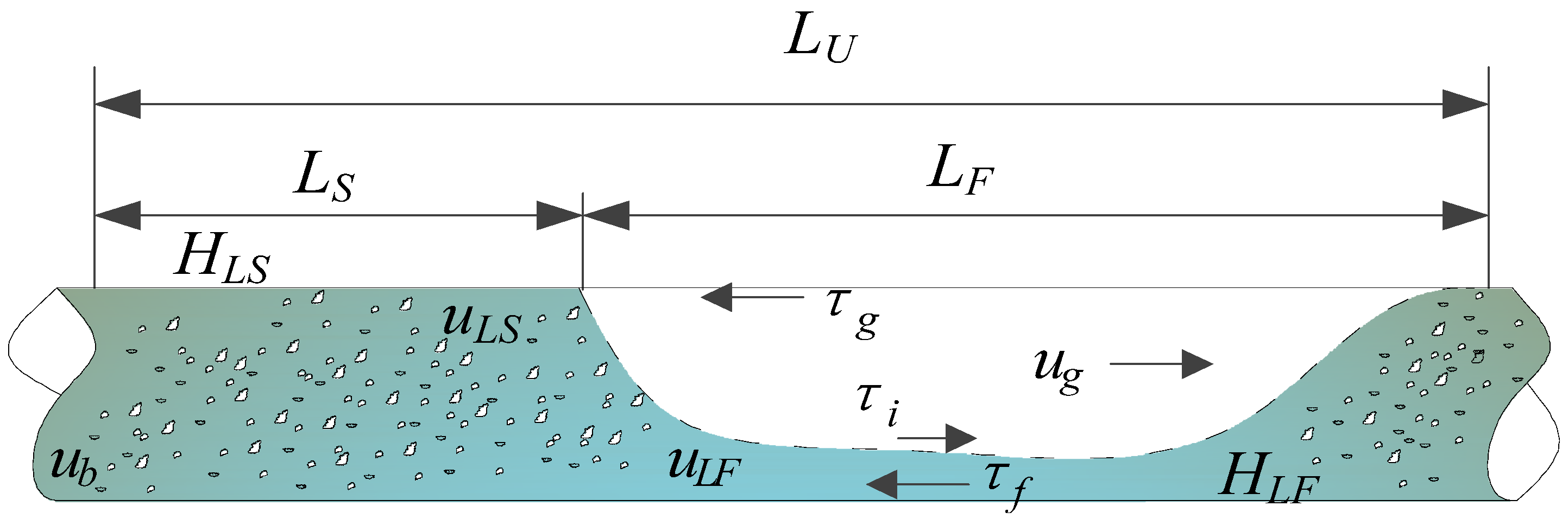
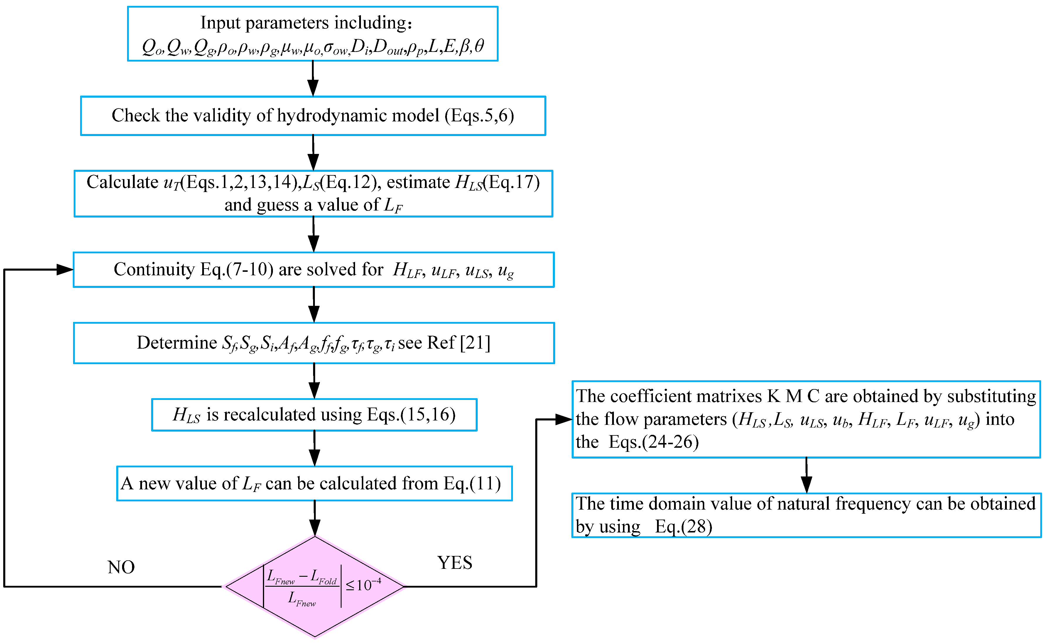
2.1. Hydrodynamic Model of Low-Viscosity Oil–Gas–Water Homogeneous Slug Flow

The distribution of the flow parameters of the low-viscosity oil–gas–water homogeneous slug flow along the pipeline should be determined before the integral calculation of the model equation.

The model was based on the following assumptions:

• That the oil-water mixture was considered homogeneous;
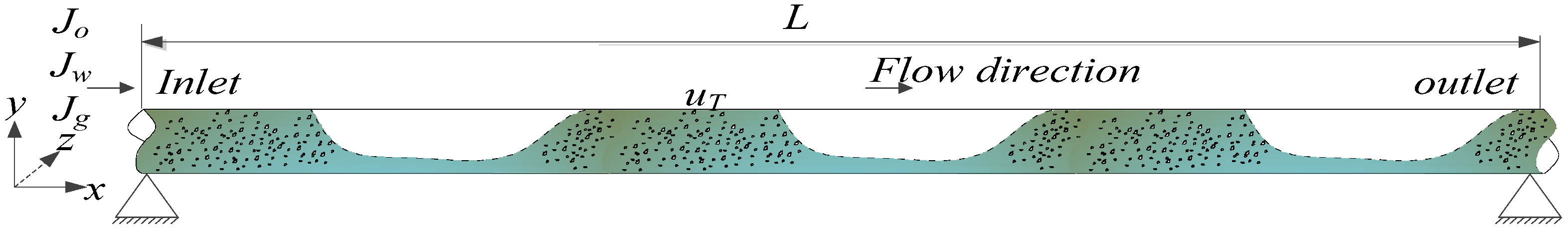
• That the slug flow was a stable flow state, with each slug unit propagating at the translational velocity (u_T) in the horizontal pipe; and
• That the oil, gas, and water were incompressible fluids.

Figure 1 shows a schematic view of the horizontal piping system conveying oil–gas–water slug flow under the simply supported boundary condition. The piping system consists of a pipe of length L with mass per unit length m_p and bending stiffness EI. The inner and outer diameters of the pipe are D_i and D_out, respectively, with D_out << L. The superficial velocities of oil, gas, and water at the inlet of the pipeline are J_o, J_g, and J_w, respectively. Several complete slug units were formed within the pipe, and the slug units propagated toward the outlet at a steady translational velocity u_T. The densities of oil, water, and gas are ρ_O, ρ_W, and ρ_G, respectively, and the corresponding dynamic viscosities are μ_O, μ_W, and μ_G.

Figure 2 shows a schematic view of a complete slug unit, which consists of a liquid slug region with length L_S and a liquid film zone with length L_F. The length of the slug unit can be denoted as L_U = L_S + L_F. The dispersed bubbles were distributed in the liquid slug region, and Taylor bubbles above the liquid film did not carry droplets. H_LS and H_LF are the liquid holdups of the liquid slug region and the liquid film zone, respectively; u_LS and u_LF are the real liquid phase velocities of the liquid slug region and the liquid film zone, respectively; u_g and u_b are the real gas velocities of the liquid slug zone and the liquid film zone, respectively.

Assuming the volume flow rates of oil, gas, and water are Q_o, Q_w, and Q_g, respectively, the corresponding superficial velocities are expressed as follows:

$$J_o=Q_o/Ai,J_w=Q_w/Ai,J_g=Q_g/Ai$$

(1)

$$J_L=J_o+J_w,J_t=J_L+J_g$$

(2)

where: J_o, J_w, and J_g, are the superficial oil, water, and gas velocities, respectively; J_L and J_t are the liquid mixture velocity and the gas–liquid mixture velocity, respectively; A_i is the cross-sectional area of the pipeline.

According to Brinkman et al. [20], the effective viscosity of oil-water homogeneous mixture based on the viscosities of the continuous phase and the dispersed phase can be calculated by the following relation:

$${\mu }_L={\mu }_{cont}{(1.0-{\Phi }_{Int})}^{-2.5}$$

(3)

where: μ_cont and μ_L are the viscosities of the continuous phase and the homogeneous mixture, respectively. Φ_Int is the volume fraction of the discrete phase. The continuous phase and discrete phase were determined by the criterion for the inversion point recommended by Zhang et al. [11].

$${\Phi }_{OI}={\left({\mu }_O/{\mu }_W\right)}^{0.4}/1+{\left({\mu }_O/{\mu }_W\right)}^{0.4}$$

(4)

where Φ_OI is the critical oil holdup in oil-water homogeneous mixture corresponding to the inversion from oil-continuous phase to water-continuous phase.

Zhang et al. [11] proposed a correlation as a criterion for distinguishing the dispersion of one fluid into another:

$$J_L>{\left(6.325Ce{\Phi }_{Int}{\left({\sigma }_{ow}\left({\rho }_w-{\rho }_o\right)\right)}^{0.5}/f_{LM}{\rho }_L\right)}^{0.5}$$

(5)

$$Ce=\left(2.5-\left|\sin \theta \right|\right)/2$$

(6)

where: θ and σ_ow are the inclination of the pipeline and the surface tension of oil and water, respectively; f_LM is the frictional factor of the liquid phase mixture; ρ_L is the density of the liquid phase mixture.

The continuity equations for the liquid phase mixture and the gas in the liquid film zone can be expressed as:

$$H_{LS}\left(u_T-u_{LS}\right)=H_{LF}\left(u_T-u_{LF}\right)$$

(7)

$$\left(1-H_{LS}\right)\left(u_T-u_b\right)=\left(1-H_{LF}\right)\left(u_T-u_g\right)$$

(8)

Definitions of the symbols used in Equations (7) and (8) can be found in Figure 2, and u_b = J_t.With the slug unit being used as the control volume, the following relationships can be derived:

$$L_U{J}_L=L_S{H}_{LS}{J}_t+L_F{H}_{LF}{u}_{LF}$$

(9)

$$L_U{J}_g=L_S\left(1-H_{LS}\right)J_t+L_F\left(1-H_{LF}\right)u_g$$

(10)

According to Zhang et al. [21], the momentum equation for the liquid film zone can be formulated as:

$$\left[{\rho }_L\left(u_T-u_{LF}\right)\left(u_{LS}-u_{LF}\right)-{\rho }_g\left(u_T-u_g\right)\left(u_b-u_g\right)\right]/L_F-{\tau }_f{S}_f/A_f+{\tau }_g{S}_g/A_g+{\tau }_i{S}_i\left(1/A_f+1/A_g\right)=0$$

(11)

where: τ_f, τ_i, and τ_g are the shear stresses of water-wall, water-gas, and gas-wall interfaces, respectively; S_f, S_g, and S_i are the wet perimeters under the action of the corresponding shear stress; A_f and A_g are the cross-sectional areas occupied by the liquid phase and by the gas phase, respectively, in the liquid film zone.

The solution of the hydrodynamic model of low-viscosity oil–gas–water homogeneous slug flow requires the following closure relation, by which the length of the liquid slug region can be estimated according to Taitel et al. [22].

$$L_S=32D_i$$

(12)

According to Nicklin [23], the translational velocity of each slug unit can be expressed as:

$$u_T=C_0{J}_t+u_D$$

(13)

where: the coefficient C₀ is taken as 1.2; u_D is the drift velocity, which can be calculated by the follow formula proposed by Bendiksen [24]:

$$u_D=0.54\sqrt{g{D}_i}$$

(14)

where: g is the acceleration of gravity.

Zhang et al. [11], based on a balance between the turbulent kinetic energy of the liquid phase and the surface free energy of the dispersed gas bubbles in a slug body, formulated the below relations:

$$H_{LS}={\left(1+T_{sm}/3.16[{\rho }_L-{\rho }_G)g\sigma {]}^{0.5}\right)}^{-1}$$

(15)

$$T_{sm}=C_e{}^{-1}\left(0.5f_s{\rho }_s{u}_s^2+0.25D_i{\rho }_L{H}_{LF}\left(u_T-u_{LF}\right)\left(J_t-u_{LF}\right)L_S{}^{-1}\right)$$

(16)

where: T_sm has the same units as shear stress and includes the wall shear stress and the contribution from the momentum exchange between the liquid slug and the liquid film in a slug unit.

The liquid slug holdup should be estimated in advance before solving other closure relationships, and the relation proposed by Gregory [25] can be employed:

$$H_{LS}={\left(1+{(J_t/8.66)}^{1.39}\right)}^{-1}$$

(17)

The frequency was calculated by the following formula:

$$fs=u_T/L_U$$

(18)

At this point, the relevant flow parameters of low-viscosity oil–gas–water homogeneous slug flow can be obtained according to the input parameters. For the specific calculation process, refer to the unified models verified by Zhang H Q et al. [26]. Zhang et al. [26] and Al-Hadhrami et al. [3] compared the experimental data with the predicted results.

2.2. Vibration Equation for Pipes Conveying Low-Viscosity Oil–Gas–Water Homogeneous Slug Flow

According to Dai [27] and Monette [28], the kinematic equation for lateral vibration of a pipe conveying low-viscosity oil–gas–water slug homogeneous flow can be expressed as:

$$EI\frac{{\partial }^{4}y}{\partial x^4}+2(m_L{u}_L+m_G{u}_G)\frac{{\partial }^{2}y}{\partial x\partial t}+(m_L{u}_L^2+m_L{u}_L^2)\frac{{\partial }^{2}y}{\partial x^2}+(m_L+m_G+m_P)\frac{{\partial }^{2}y}{\partial t^2}=0$$

(19)

where: EI is flexural rigidity; m_P, m_G, and m_L are the masses of pipe, air, and liquid mixture per unit length, respectively; u_G and u_L are severally located gas and liquid flow velocities; y is the transverse displacement of the pipe.

For the convenience of solution, high-order partial differential Equation (19) was discretized and reduced into a low-order ordinary differential equation by Galerkin’s method and orthogonal modal properties. According to modal orthogonality, the transverse displacement of the pipeline can be expressed as follows:

$$y={\displaystyle {\sum }_j^N\left({\phi }_j\left(x\right)q_j\left(t\right)\right)}={\Phi }^{T}q$$

(20)

where: φ_j (x) is the vibration mode function (i.e., eigenfunction) given by Equation (21); q_j(t) is the generalized coordinate; N is the order. In this article, two-order vibration was considered, so N was taken as 2.

$${\Phi }^T={\left(\sin (\pi x/L),\sin (2\pi x/L)\right)}^T$$

(21)

Substituting Equation (20) into Equation (19) gives the following equation:

$$EI{\Phi }^{(4)T}q+2(m_L{u}_L+m_G{u}_G){{\Phi }^{\prime }}^T\dot{q}+(m_L{u}_L^2+m_L{u}_L^2){{\Phi }^{″}}^{T}q+(m_L+m_G+m_P){\Phi }^T\ddot{q}=0$$

(22)

Left-multiplying Equation (22) by Φ and integrating it in the interval [0, L] along the pipe length gives:

$${\displaystyle {\int }_0^{L}EI\Phi {\Phi }^{(4)T}q}dx+{\displaystyle {\int }_0^{L}2(m_L{u}_L+m_G{u}_G)\Phi {{\Phi }^{\prime }}^T\dot{q}dx}+{\displaystyle {\int }_0^L(m_L{u}_L^2+m_L{u}_L^2)\Phi {{\Phi }^{″}}^{T}qdx}+{\displaystyle {\int }_0^L(m_L+m_G+m_P)\Phi {\Phi }^T\ddot{q}}dx=0$$

(23)

Express the coefficient matrices M, C, and K as:

$$M={\displaystyle {\int }_0^L(m_L+}{m}_G+m_P)\Phi {\Phi }^{T}dx$$

(24)

$$C={\displaystyle {\int }_0^{L}2(m_L{u}_L+}{m}_G{u}_G)\Phi {{\Phi }^{\prime }}^{T}dx$$

(25)

$$K={\displaystyle {\int }_0^{L}EI\Phi {\Phi }^{(4)}{}^{T}dx}+{\displaystyle {\int }_0^L(m_L{u}_L^2+}{m}_G{u}_G^2)\Phi {{\Phi }^{″}}^{T}dx$$

(26)

where M is the mass matrix; C is the fluid–structure coupling damping matrix; K is the stiffness matrix.

It should be noted that m_L = ρ_LA_iH_L, and m_G = ρ_GA_i(1 − H_L), where H_L is the local liquid holdup, a function of coordinate x and time t. Other parameters such as u_L and u_G are also functions of coordinate x and time t. All these are denoted as H_L(x, t), u_L(x, t), and u_G(x, t), respectively. However, the integral calculation in Equations (24)–(26) within the interval (0, L] should be done piecewise, due to the intermittent characteristics of slug flow. Reference [17] presents the method of integral interval segmentation and the concrete integral formulae for coefficient matrices M, C, and K.

Equation (23) is further simplified as follows:

$$M(t)\ddot{q}(t)+C(t)\dot{q}(t)+K(t)q(t)=0$$

(27)

Equation (27) can determine the natural frequency of the pipeline conveying flow by solving for the eigenvalues of matrix E(t).

$$E(t)=\left[\begin{array}{cc}0& I\\ -M{(t)}^{-1}K(t)& -M{(t)}^{-1}C(t)\end{array}\right]$$

(28)

where I is identity matrix.

The eigenvalues of matrix E(t) can be expressed in the following complex form:

$$\Gamma \left(t\right)=R\left(t\right)+\omega \left(t\right)i$$

(29)

The imaginary part ω(t) of the eigenvalues represents the natural frequency. The basic calculation process goes as follows: first, the flow parameters are obtained based on the hydrodynamic model; next, the relevant parameters are fed into the fluid–structure interaction dynamics model, the coefficient matrices M, C, and K are calculated, and the time-domain values of the pipe’s natural frequency can be derived from Equation (28). The specific calculation process is shown in Figure 3.

3. Results and Discussion

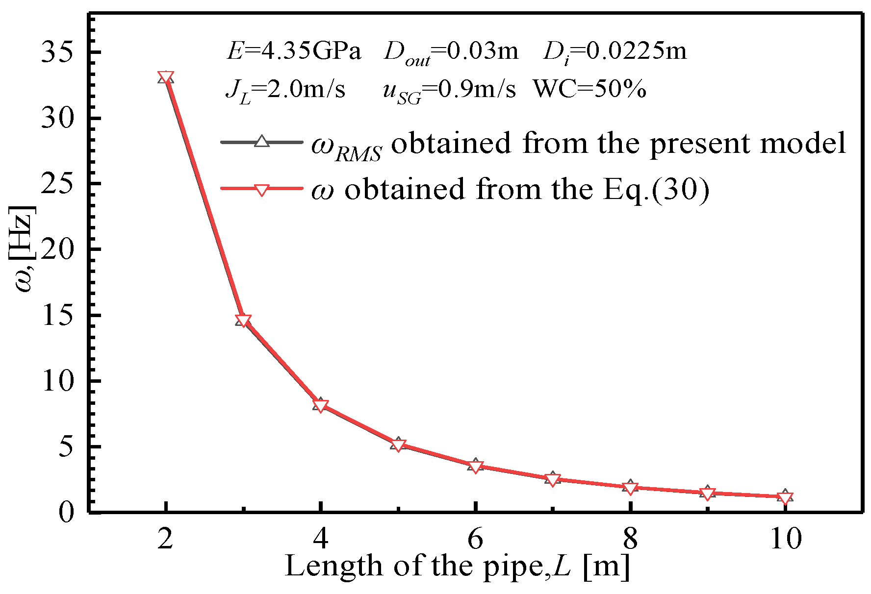
3.1. Model Validation

Liu et al. [17] confirmed that the natural frequency of piping systems conveying slug flow with high liquid holdup was quite close to that of piping systems conveying single-phase flow. The same method was used to validate the present model.

Before the model validation, some basic parameters needed to be set in advance. In this article, the inner and outer diameters of the pipe are 0.0225 m and 0.030 m, respectively. Young’s modulus E is 4.35 GPa, and pipe density ρ_p is 1180 kg/m³. The viscosities of water, oil, and gas are 1 Pa·s, 1.77 Pa·s, and 0.00179 Pa·s, respectively. The densities of water, oil, and gas are 998 kg/m³, 800 kg/m³, and 1.25 kg/m³, respectively. The oil-water surface tension is 0.042 N/m.

Under the simply supported boundary condition, the first-order natural frequency of piping systems conveying single-phase flow was modeled as follows [6]:

$${\omega }_1={\beta }^2\sqrt{EI/\left(m_p+m_f\right)}\sqrt{1-m_f{u}^2/EI{\beta }^2}$$

(30)

where β = π/L; u is fluid velocity; m_f is mass of fluid per unit length. It is worth noting that m_f and u are scalars. Due to the large difference between gas density and liquid density, the gas mass was ignored. Therefore, m_f can be calculated by the following formula:

$$m_f={\rho }_{L}HAi$$

(31)

Figure 4 shows the distribution profile of liquid holdup and liquid velocity at J_L = 2.0 m/s, J_g = 0.9m/s, and WC = 50%. Under this condition, the length of the liquid film zone is much shorter than the length of the liquid slug region and the liquid holdup is relatively high. The liquid velocity distribution along the pipe is similar to the liquid holdup distribution, which means that the slug flow corresponding to this flow condition could be treated approximately as if only water with equivalent area flowed in the pipe. According to Liu et al. [17], J_t was employed as the fluid velocity(u), and the relevant formula is given as follows:

$$H=\left(H_{LS}{L}_S+H_{LF}{L}_F\right)/L_U$$

(32)

where H is the average liquid holdup of each slug unit.

The intermittent characteristics of slug flow led to the periodic motion of natural frequency, so the piping system’s natural frequency is represented in terms of its root mean square (RMS). Figure 5 shows the comparison between the natural frequencies predicted by the present model and the calculated results from Equation (30) at distinct pipe lengths. It is worth noting that the RMS value of the natural frequencies calculated by the present model is in good agreement with the result calculated by Equation (30) at each pipe length.

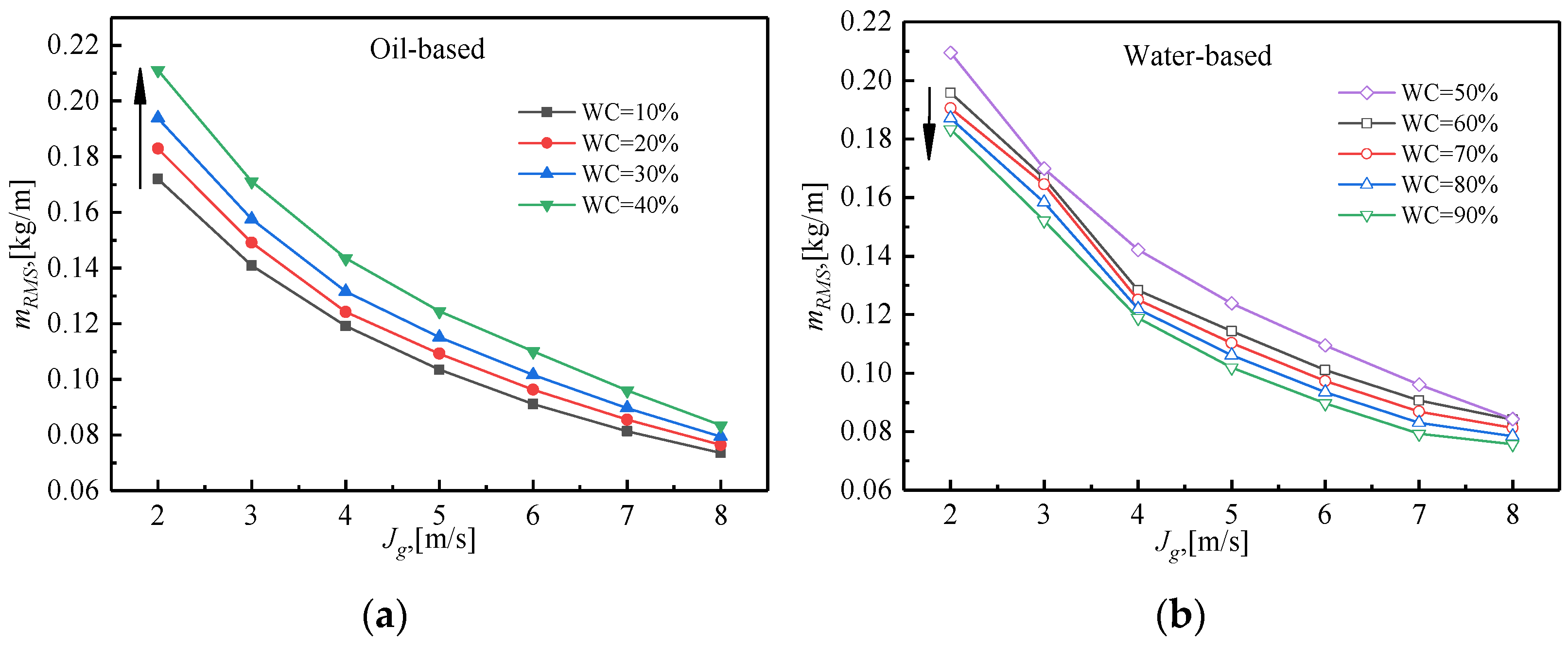
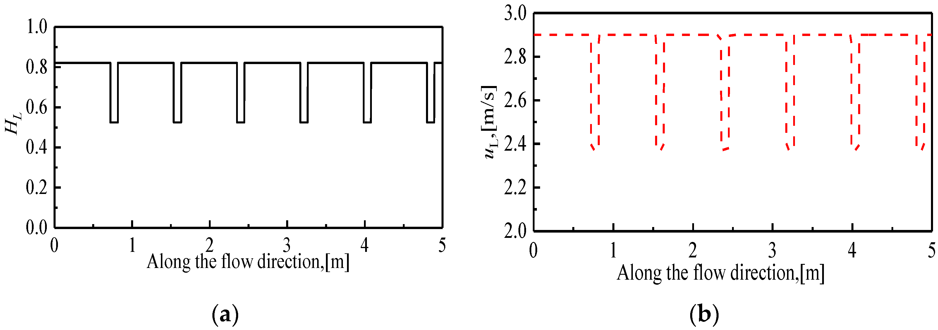
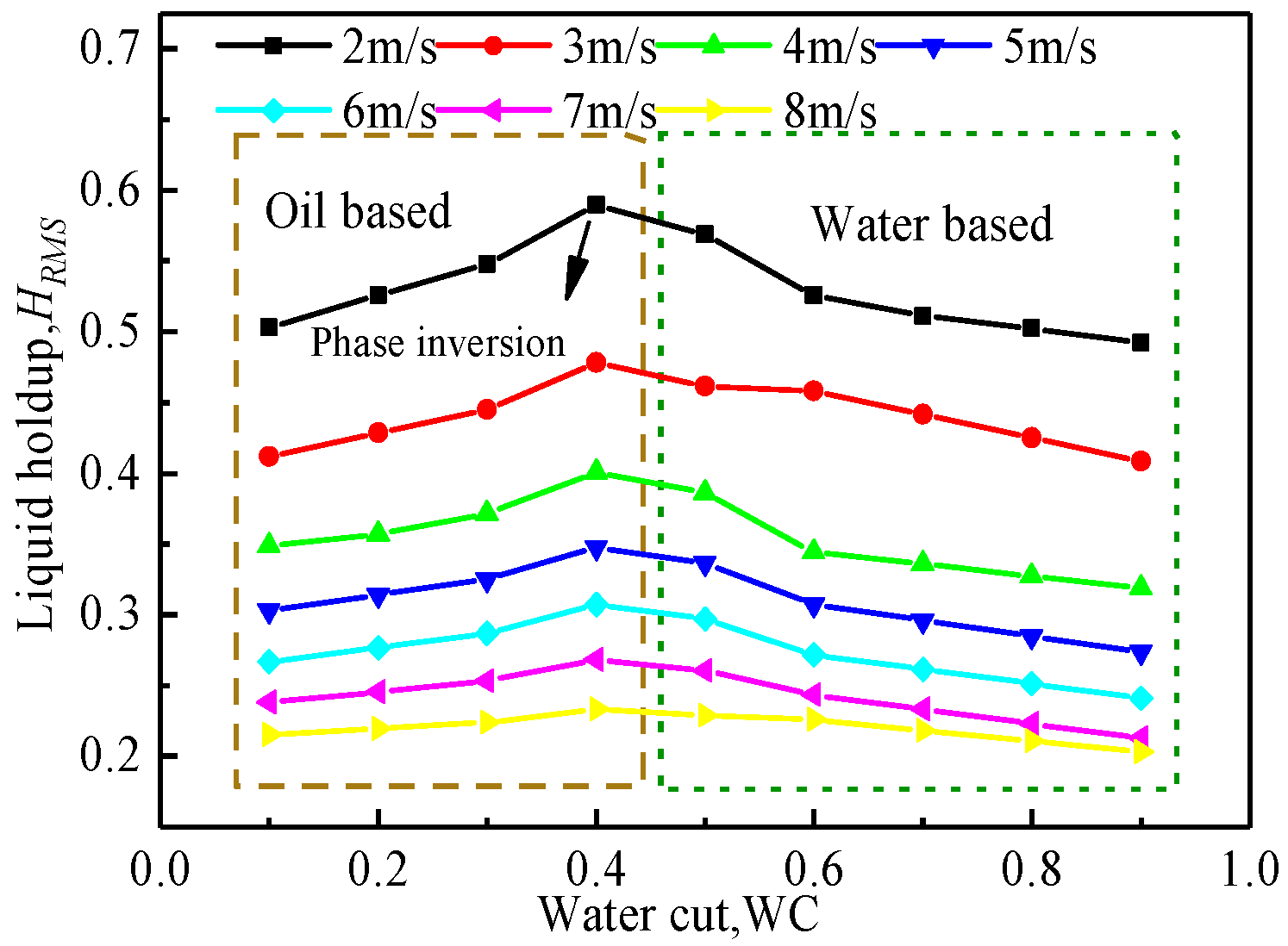
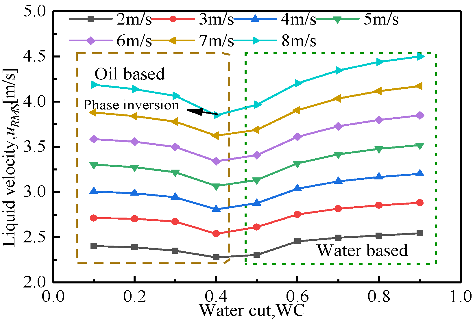
3.2. Effect of WC on Liquid Holdup and Liquid Velocity

To ensure that the flow regimes studied were slug flow, the superficial liquid and gas velocities were selected as 0.8–1.5 m/s and 2.0–8.0 m/s, respectively, with WC = 10–90%, according to the experimental data in reference [3].

The behaviors of the internal fluid have a significant influence on the vibration of the piping system. The liquid holdup and liquid velocity change periodically, as can be seen in Figure 4. To characterize how the liquid holdup and liquid velocity vary with WC and superficial gas velocity, both parameters are denoted in terms of their RMS value within one period as H_RMS and u_RMS, respectively.

The variations of liquid holdup with WC and superficial gas velocity are shown in Figure 6. The liquid holdup increases first and then decreases with WC at distinct superficial gas velocities, peaking near the phase inversion point. According to Equation (4), the continuous phase inversion from oil to water occurs at Φ_OI = 55.7%. In this article, the oil-based slug flow occurs within the range of 10–40% WC, whereas the water-based slug flow occurs at the range of 50–90% WC. According to Equation (3), the effective viscosity of the homogeneous mixture increases with the increase in WC in the oil-based slug flow regime, whereas it decreases with the increase in WC in the water-based slug flow regime. The effective viscosity reaches the maximum in the phase inversion region. This accounts for the maximum of liquid holdup at WC = 40% followed by a gradual decrease in the water-based slug flow region. The difference between the liquid holdup corresponding to phase inversion point and others diminished with the increase in the superficial gas velocity, due primarily to the inertia force increasing with the increase in the superficial gas velocity, which counteracts the effect of viscosity. However, the total liquid holdup remains almost the same with the maximum percentage of 10% for the whole range of WC. Similar conclusions were also drawn in Reference [29].

The liquid velocity variations with WC for J_L = 1.5m/s and J_g = 2.0–8.0 m/s are shown in Figure 7. It can be seen that the liquid velocity u_RSM decreases first and then increases with the increase in WC and that it reaches the minimum in the phase inversion region. This trend is opposed to that of the liquid holdup. In the oil-based slug flow regime, the effective viscosity increases with the increase in WC, which leads to the decrease in liquid velocity. However, the opposite trend occurs in the water-based slug flow regime. This also means that in the water-based slug flow regime, the water phase acts as a lubricant that reduces the viscous force between the liquid and the wall.

Figure 8 shows the internal liquid fluid mass per unit length (m_RMS) varying with WC for J_L = 1.5 m/s and J_g = 2.0–8.0 m/s. As can be seen from Figure 8a, m_RMS increases as WC increases at each superficial gas velocity, due primarily to both the liquid holdup and mixture density increasing with the increase in WC. Furthermore, it is worth noting that the difference between the values of m_RSM of different WC decreases as J_g increases.

In the water-based slug flow regime (See Figure 8b), m_RMS decreases as WC increases. The variation of H_RMS in Figure 6 can be easily understood as a result of density difference. Comparing Figure 8a,b, m_RMS shows opposite variation trends in the oil-based and the water-based slug flow states with the increase in WC. Obviously, the increase in m_RMS in the oil-based slug flow regime is the result of the positive effect of liquid holdup and mixture density. Whereas the change of mixture density is positive, the change of liquid holdup is negative in the water-based slug flow regime. It can be concluded from the results that the influence of liquid holdup rate is responsible for the change of m_RMS in water-based slug flow. The variation of m_RSM with WC has a significant influence on the natural frequency. Liu et al. [17] stated that the decrease in liquid mass per unit length (m_L) and liquid velocity (u_L) was beneficial for the increase in natural frequency. This is helpful for the analysis on the change of natural frequency with WC and superficial gas velocity.

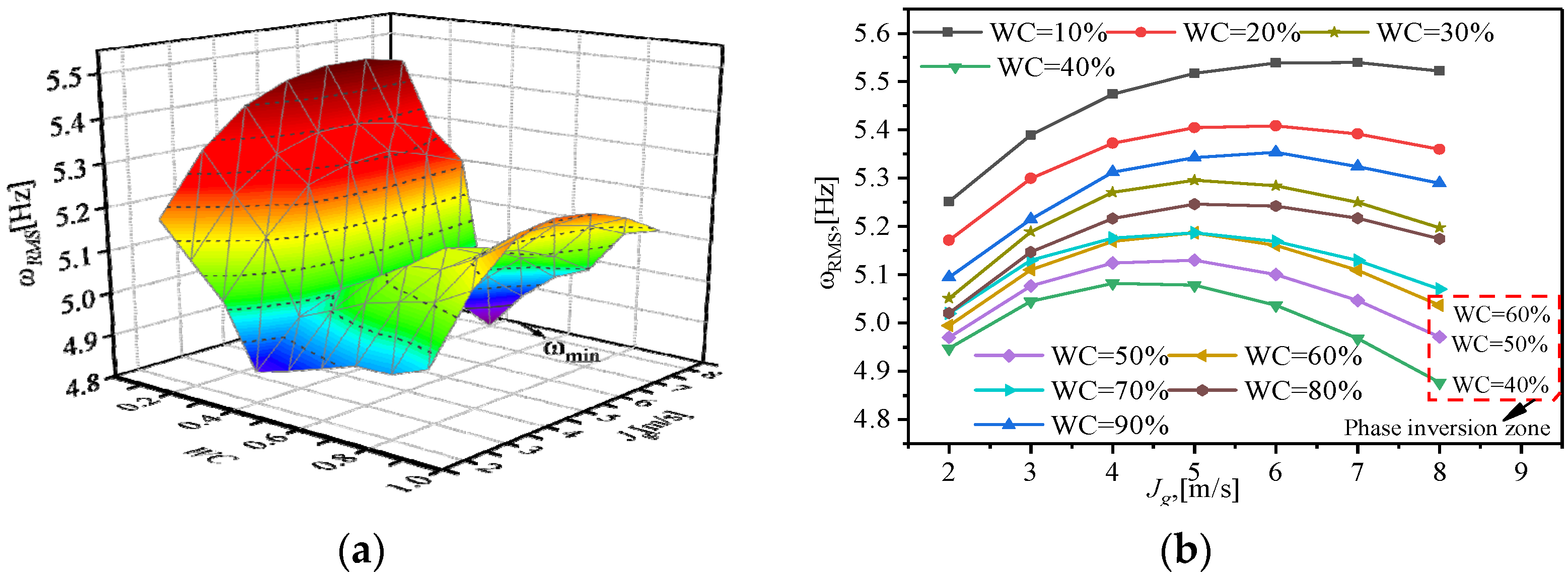
3.3. Effect of WC on Natural Frequency

Figure 9 depicts the influence of WC and superficial gas velocity on natural frequency of the piping system. Figure 9a shows that the natural frequency varies with the WC and superficial gas velocity and presents characteristics similar to a ‘saddle surface’. The natural frequency decreases first and then increases with the increase in WC, and the ‘saddle point’ appears near the phase inversion point due to the maximum liquid holdup in the phase inversion zone. The minimum natural frequency appears at the flow condition of J_g = 8.0 m/s and WC = 40%. The maximum natural frequency appears in the high superficial gas velocity zone because of the relative low mass per unit length of the fluid. As can be seen from Figure 9b, the natural frequencies near the phase inversion region (WC = 40–60%) are relatively low. In the oil-based slug flow regime (WC ≤ 40%), the natural frequency decreases with the increase in WC, whereas in the water-based slug flow regime, the natural frequency increases with the increase in WC.

In the oil-based slug flow regime, the viscosity and density of the homogeneous mixture increase with the increase in WC, whereas the liquid velocity decreases and the liquid holdup increases with the increase in viscosity (See Figure 6 and Figure 7). The liquid mass per unit length increases with the increase in density and liquid holdup (See Figure 8a). The liquid velocity and liquid mass per unit length show opposite trends with the increase in WC. According to Liu et al. [17], the change of natural frequency with WC depends on which of them is dominant. The results showed that the liquid mass per unit length was the dominant influencing factor (See Figure 9b).

In the water-based slug flow regime, the viscosity of the homogeneous mixture increases with the increase in WC and so does the density of the homogeneous mixture, whereas the liquid velocity decreases and the liquid holdup increases with the increase in viscosity (see Figure 6 and Figure 7). The liquid mass per unit length increases with the increase in density and liquid holdup (See Figure 8b). The liquid velocity and liquid mass per unit length show opposite trends with the increase in WC. The results showed that the liquid mass per unit length is the dominant influencing factor (See Figure 9b). By comparing the mathematical relations of μ_L, ρ_L, u_RMS, and H_RMS with WC, it can be seen that the influence of WC on μ_L is the dominant factor leading to the variation of natural frequency in both slug flow regimes.

It can be seen that the increase in WC is unfavorable in the oil-based slug flow regime and that the most unfavorable point is near the phase inversion point, whereas the increase in WC is favorable in the water-based slug flow regime. In addition, the natural frequency increases first and then decreases with the increase in superficial gas velocity, indicating that there is a critical gas velocity. It is worth noting that the superficial gas velocity corresponding to the natural frequency beginning to decline in the oil-based slug flow regime decreases from 7 m/s at WC = 10% to 4 m/s at WC = 40% with the increase in WC from 10% to 40%. The opposite trend occurs in the water-based slug flow regime, namely an increase from 5 m/s at WC = 50% to 6 m/s at WC = 90%.

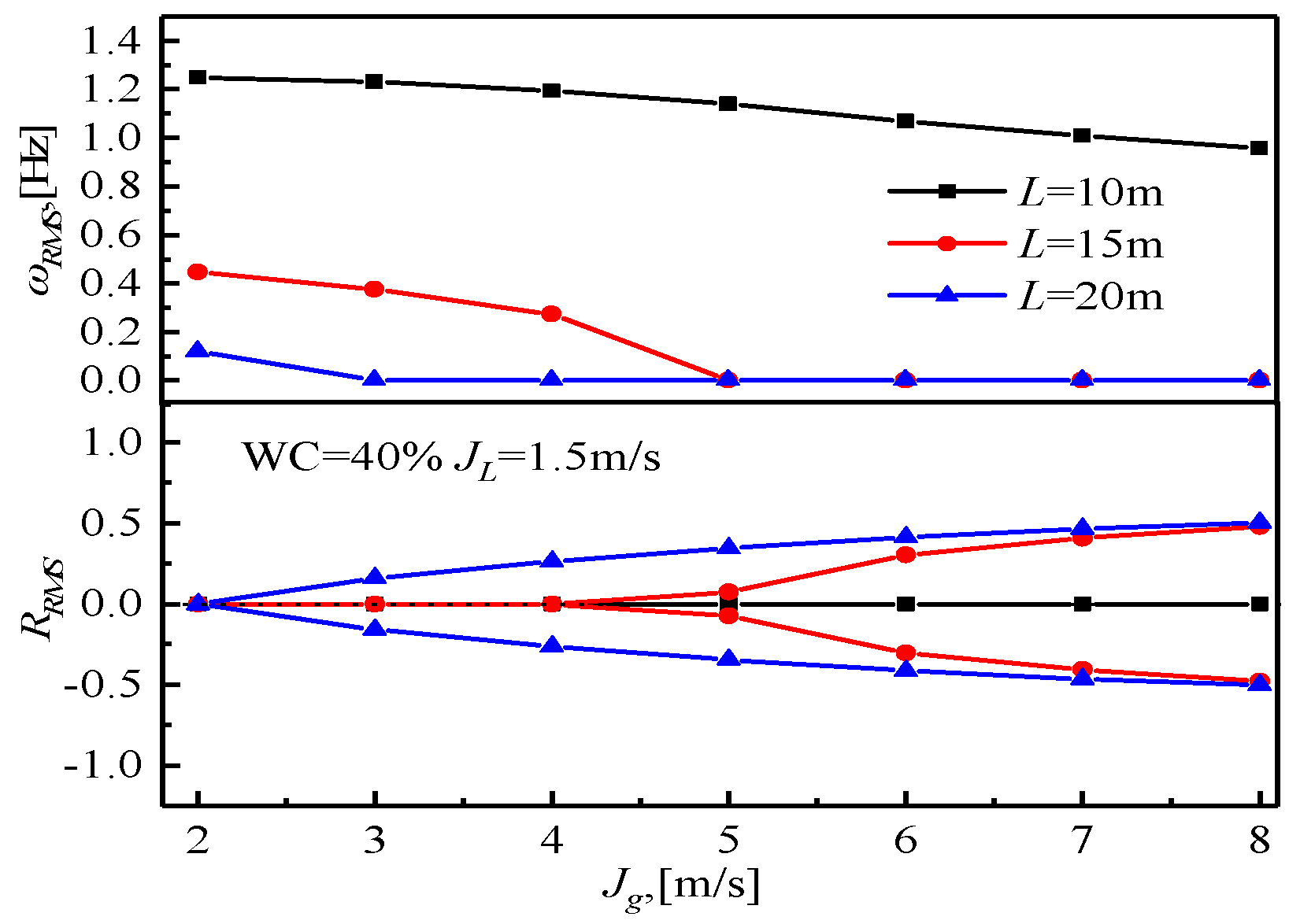
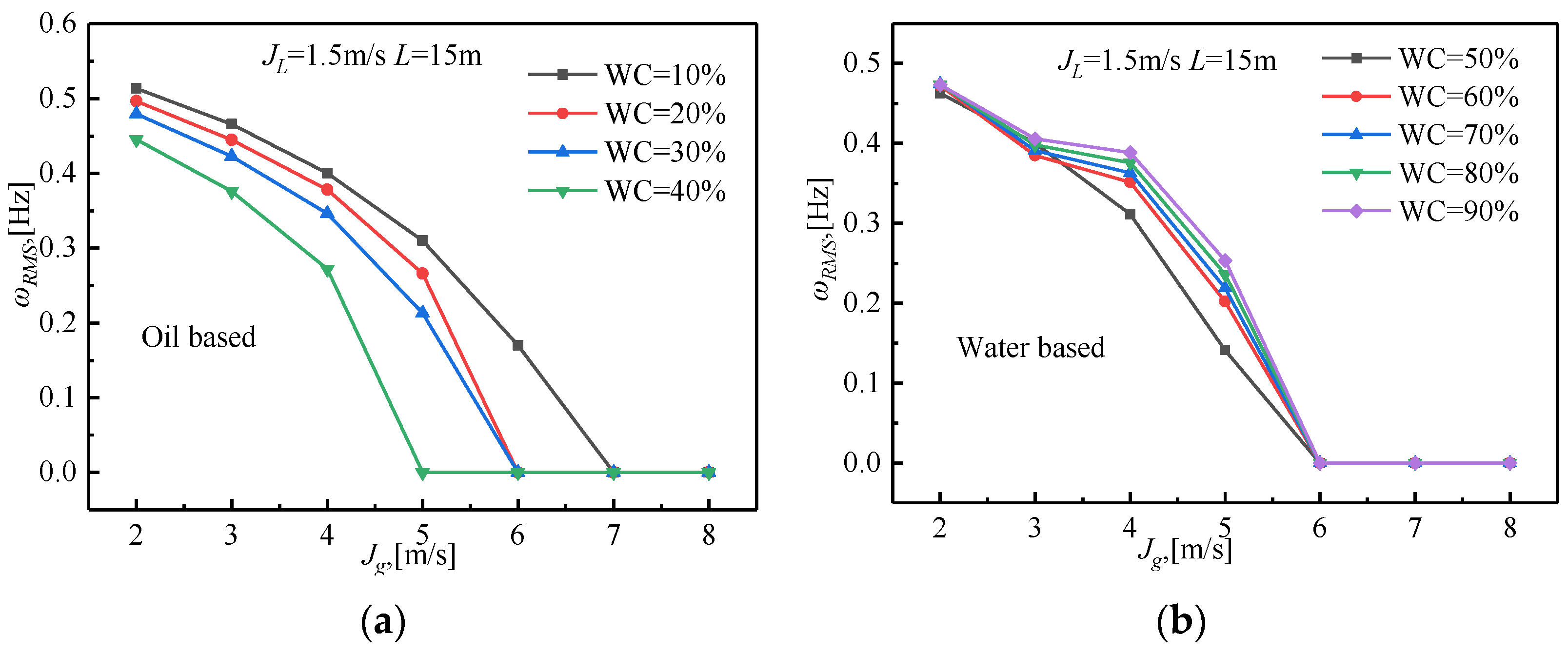
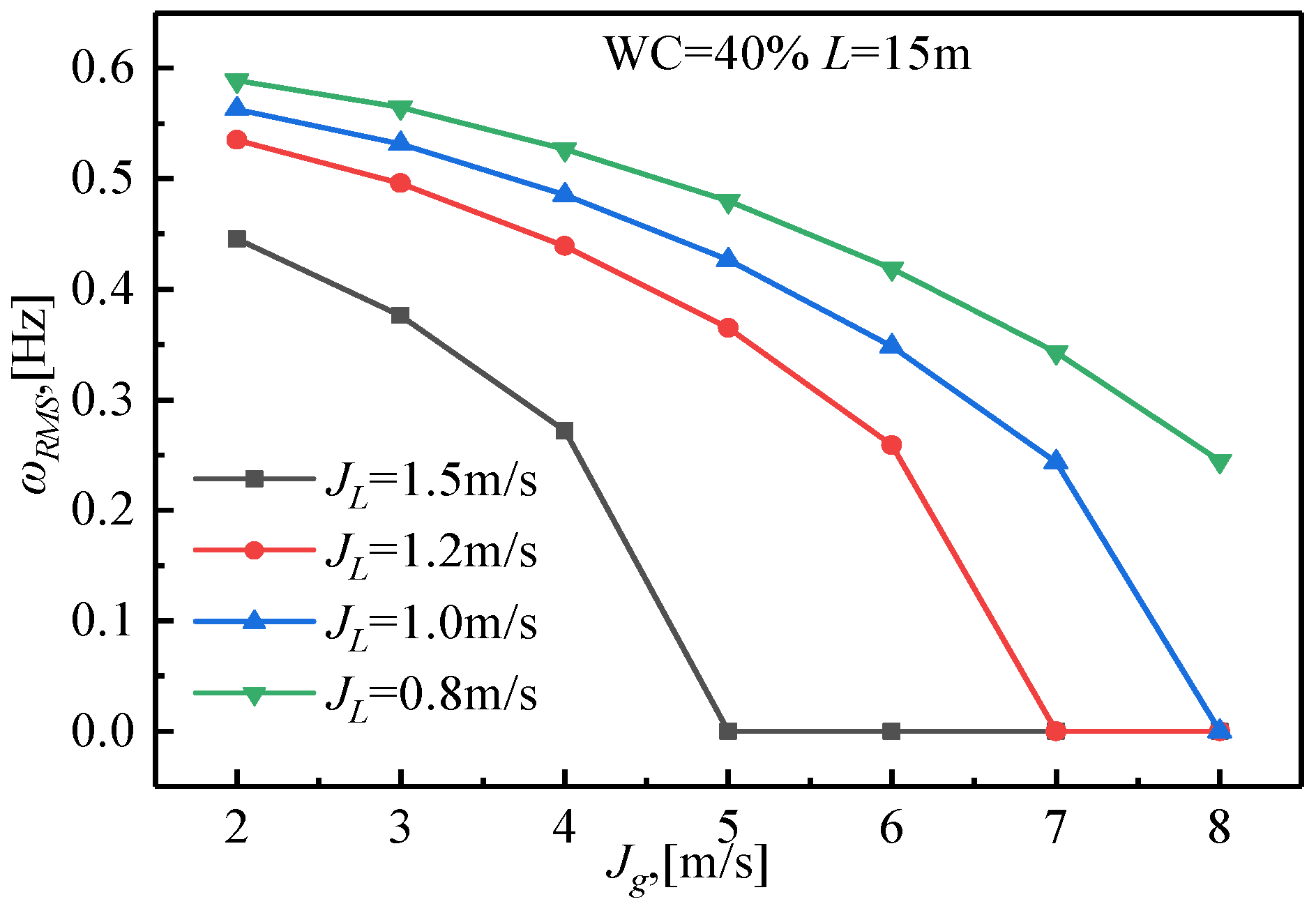
3.4. Influencing Factors of the Critical Gas Velocity

Figure 10 shows the variation of the real and imaginary parts of the first-order natural frequency with pipe length and superficial gas velocity for WC = 40% and J_L = 1.5 m/s. When the pipeline length is 10 m, the natural frequency decreases with the increase in superficial gas velocity, corresponding to the real part of the eigenvalue Γ = 0 for the whole range of superficial gas velocity. This means that the pipe was statically stable. As the pipe length increases to 15 m, the natural frequency decreases to zero whereas the superficial gas velocity increases to 5 m/s. The real part of the eigenvalue becomes two curves with one being negative and the other being positive when the superficial gas velocity exceeds 5 m/s, which indicates a divergent instability according to Paidoussis and Issid [30]. As the pipeline length further increases to 20 m, the critical gas velocity decreases to 3 m/s. A comparison of the changes of the critical gas velocity at distinct pipe lengths reveals that the critical gas velocity decreases with the increase in pipe length.

As can be seen from Figure 11a, the critical gas velocity is equal to 7 m/s at WC = 10% and that as WC increases to 40%, the critical gas velocity decreases to 5 m/s. However, in the water-based slug flow state, WC has little effect on the critical gas velocity, which is 6 m/s within the range of 50–90% WC, as can be seen in Figure 11b. The minimum critical gas velocity occurs at WC = 40%. In order to ensure the stable operation of the pipeline, it is necessary to avoid the flow conditions near the phase inversion zone.

In addition, the superficial liquid velocity has a great influence on the critical gas velocity. As can be seen from Figure 12, the critical gas velocity is absent in the whole range of superficial gas velocity for J_L = 0.8 m/s. The critical gas velocities corresponding to J_L = 1.0 m/s, J_L = 1.2 m/s, and J_L = 1.5 m/s are 8 m/s, 7 m/s, and 5 m/s, respectively. Evidently, the critical gas velocity tends to decline with the increase in superficial liquid velocity.

4. Conclusions

In this study, a new model of horizontal pipes conveying low-viscosity oil–gas–water slug flow is established. The effects of water cut (WC) and superficial gas velocity on natural frequency are analyzed. The following conclusions are drawn.

In the oil-based slug flow regime, the natural frequency decreases with the increase in WC, whereas in the water-based flow regime (WC = 50–90%), the natural frequency decreases with the increase in WC. Compared with other WCs, when the WC = 40% (near the phase transition point) the natural frequency reaches the minimum. The relationship between effective viscosity and WC in both flow regimes is the fundamental reason for the variation of natural frequency.

The natural frequency increases first and then decreases with the increase in superficial gas velocity. The turning point in the oil-based slug flow regime decreases from 7 m/s at WC = 10% to 4 m/s at WC = 40%, whereas in the water-based slug flow regime, it increases from 5 m/s at WC = 50% to 6 m/s at WC = 90%. It has been indicated that there is a critical gas velocity related to the pipe length, superficial liquid velocity, and WC.

The increase in superficial liquid velocity has resulted in an increase in liquid mass per unit length, thus causing a decrease in the critical gas velocity. In the oil-based slug flow regime, the critical gas velocity decreases with the increase in WC. However, in the water-based regime, WC has little influence on the critical gas velocity. Nevertheless, it is necessary to fully analyze the combined effect of slug parameters m_RMS and u_RMS and the geometric parameters of the pipe to determine the critical gas velocity. By investigating the effect of WC on the vibration characteristics of the piping system, conveying low viscosity oil–gas–water slug flow can provide guidance for operational and design safety.

References

1. Paıdoussis, M.; Li, G. Pipes conveying fluid: A model dynamical problem. J. Fluids Struct. 1993, 7, 137–204. [Google Scholar] [CrossRef]
2. Miwa, S.; Mori, M.; Hibiki, T. Two-phase flow induced vibration in piping systems. Prog. Nucl. Energy 2015, 78, 270–284. [Google Scholar] [CrossRef]
3. Al-Hadhrami, L.M.; Shaahid, S.; Tunde, L.O.; Al-Sarkhi, A. Experimental study on the flow regimes and pressure gradients of air-oil-water three-phase flow in horizontal pipes. Sci. World J. 2014, 2014, 1–11. [Google Scholar] [CrossRef] [PubMed] [Green Version]
4. Rahmanian, M.; Firouz-Abadi, R.; Cigeroglu, E. Dynamics and stability of conical/cylindrical shells conveying subsonic compressible fluid flows with general boundary conditions. Int. J. Mech. Sci. 2017, 120, 42–61. [Google Scholar] [CrossRef]
5. Wang, L. A further study on the non-linear dynamics of simply supported pipes conveying pulsating fluid. Int. J. Non-Linear Mech. 2009, 44, 115–121. [Google Scholar] [CrossRef]
6. Huang, Y.-M.; Liu, Y.-S.; Li, B.-H.; Li, Y.-J.; Yue, Z.-F. Natural frequency analysis of fluid conveying pipeline with different boundary conditions. Nucl. Eng. Des. 2010, 240, 461–467. [Google Scholar]
7. Wang, L.; Dai, H.; Qian, Q. Dynamics of simply supported fluid-conveying pipes with geometric imperfections. J. Fluids Struct. 2012, 29, 97–106. [Google Scholar] [CrossRef]
8. Liu, Y.; Miwa, S.; Hibiki, T.; Ishii, M.; Morita, H.; Kondoh, Y.; Tanimoto, K. Experimental study of internal two-phase flow induced fluctuating force on a 90 elbow. Chem. Eng. Sci. 2012, 76, 173–187. [Google Scholar] [CrossRef]
9. An, C.; Su, J. Vibration behavior of marine risers conveying gas-liquid two-phase flow. In International Conference on Offshore Mechanics and Arctic Engineering; American Society of Mechanical Engineers: New York City, NY, USA, 2015; p. V05AT4A016. [Google Scholar]
10. Giraudeau, M.; Mureithi, N.; Pettigrew, M. Two-phase flow-induced forces on piping in vertical upward flow: Excitation mechanisms and correlation models. J. Press. Vessel. Technol. 2013, 135, 030907. [Google Scholar] [CrossRef]
11. Zhang, H.-Q.; Sarica, C. Unified Modeling of Gas/Oil/Water-Pipe Flow-Basic Approaches and Preliminary Validation. SPE Proj. Facil. Constr. 2006, 1, 1–7. [Google Scholar] [CrossRef]
12. Zhao, J.M.; Gong, J.; Yu, D. Oil-Gas-Water Three-Phase Slug Flow Liquid Holdup Model in Horizontal Pipeline. In Proceedings of the International Pipeline Conference, Calgary, AB, Canada, 25–29 September 2006; pp. 183–190. [Google Scholar]
13. Dehkordi, P.B.; Colombo, L.; Mohammadian, E.; Shahrabadi, A.; Azdarpour, A. A mechanistic model to predict pressure drop and holdup pertinent to horizontal gas-liquid-liquid intermittent flow. Chem. Eng. Res. Des. 2019, 149, 182–194. [Google Scholar] [CrossRef] [Green Version]
14. Meng, S.; Chen, Y.; Che, C. Slug flow’s intermittent feature affects VIV responses of flexible marine risers. Ocean. Eng. 2020, 205, 106883. [Google Scholar] [CrossRef]
15. Azevedo, G.; Baliño, J.; Burr, K. Influence of pipeline modeling in stability analysis for severe slugging. Chem. Eng. Sci. 2017, 161, 1–13. [Google Scholar] [CrossRef]
16. Khudayarov, B.; Komilova, K.M. Vibration and dynamic stability of composite pipelines conveying a two-phase fluid flows. Eng. Fail. Anal. 2019, 104, 500–512. [Google Scholar] [CrossRef]
17. Liu, G.; Wang, Y. Study on the natural frequencies of pipes conveying gas-liquid two-phase slug flow. Int. J. Mech. Sci. 2018, 141, 168–188. [Google Scholar] [CrossRef]
18. Zhong, Q.; Luo, Z. Coupled vibration response of marine riser caused by oil-gas-water three-phase slug flow. Chin. J. Eng. Des. 2019, 26, 95–101. [Google Scholar]
19. Yaqub, M.W.; Marappagounder, R.; Rusli, R.; DM, R.P.; Pendyala, R. Review on gas–liquid–liquid three–phase flow patterns, pressure drop, and liquid holdup in pipelines. Chem. Eng. Res. Des. 2020, 159, 505–528. [Google Scholar] [CrossRef]
20. Brinkman, H.C. The viscosity of concentrated suspensions and solutions. J. Chem. Phys. 1952, 20, 571. [Google Scholar] [CrossRef]
21. Zhang, H.-Q.; Wang, Q.; Sarica, C.; Brill, J.P. Unified model for gas-liquid pipe flow via slug dynamics—Part 1: Model development. J. Energy Resour. Technol. 2003, 125, 266–273. [Google Scholar] [CrossRef]
22. Taitel, Y.; Barnea, D.; Dukler, A. Modelling flow pattern transitions for steady upward gas-liquid flow in vertical tubes. AIChE J. 1980, 26, 345–354. [Google Scholar] [CrossRef]
23. Nicklin, D. Two-phase bubble flow. Chem. Eng. Sci. 1962, 17, 693–702. [Google Scholar] [CrossRef]
24. Bendiksen, K.H. An experimental investigation of the motion of long bubbles in inclined tubes. Int. J. Multiph. Flow 1984, 10, 467–483. [Google Scholar] [CrossRef] [Green Version]
25. Gregory, G.; Nicholson, M.; Aziz, K. Correlation of the liquid volume fraction in the slug for horizontal gas-liquid slug flow. Int. J. Multiph. Flow 1978, 4, 33–39. [Google Scholar] [CrossRef]
26. Zhang, H.-Q.; Wang, Q.; Sarica, C.; Brill, J.P. Unified model for gas-liquid pipe flow via slug dynamics—Part 2: Model validation. J. Energy Resour. Technol. 2003, 125, 274–283. [Google Scholar] [CrossRef]
27. Dai, H.; Wang, L.; Ni, Q. Dynamics of a fluid-conveying pipe composed of two different materials. Int. J. Eng. Sci. 2013, 73, 67–76. [Google Scholar] [CrossRef]
28. Monette, C.; Pettigrew, M. Fluidelastic instability of flexible tubes subjected to two-phase internal flow. J. Fluids Struct. 2004, 19, 943–956. [Google Scholar] [CrossRef]
29. Wang, S.; Zhang, H.-Q.; Sarica, C.; Pereyra, E. Experimental study of high-viscosity oil/water/gas three-phase flow in horizontal and upward vertical pipes. SPE Prod. Oper. 2013, 28, 306–316. [Google Scholar] [CrossRef]
30. Paidoussis, M.P.; Issid, N. Dynamic stability of pipes conveying fluid. J. Sound Vib. 1974, 33, 267–294. [Google Scholar] [CrossRef]
Figure 1. Schematic view of a pipe conveying oil–gas–liquid slug flow.
Processes 10 00992 g001
Figure 2. Schematic view of a complete slug unit.
Processes 10 00992 g002
Figure 3. The flowchart of numerical evaluations in this work.
Processes 10 00992 g003
Figure 4. Distributions of liquid holdup and liquid velocity along the pipe for JL = 2.0 m/s, Jg = 0.9 m/s, and WC = 50%. (a) Distribution of liquid holdup; (b) Distribution of liquid velocity.
Processes 10 00992 g004
Figure 5. Comparison between natural frequencies determined from the present model and Equation (30).
Processes 10 00992 g005
Figure 6. HRSM variation with WC at JL = 1.5 m/s, Jg = 2.0–8.0 m/s.
Processes 10 00992 g006
Figure 7. uRSM variation with WC at JL = 1.5 m/s, Jg = 2.0–8.0 m/s.
Processes 10 00992 g007
Figure 8. mRSM variation with WC at JL = 1.5 m/s, Jg = 2.0–8.0 m/s: (a) Oil-based; (b) Water-based.
Processes 10 00992 g008
Figure 9. Effect of WC and Jg on natural frequency at JL = 1.5 m/s: (a) The cloud diagram of natural frequency variation with WC and Jg; (b) Natural frequency variation with Jg.
Processes 10 00992 g009
Figure 10. Variations of ωRMS and RRMS with Jg and L in the first mode.
Processes 10 00992 g010
Figure 11. Variation of the critical gas velocity with WC: (a) Oil-based; (b) Water-based.
Processes 10 00992 g011
Figure 12. Variation of the critical gas velocity with superficial liquid velocity.
Processes 10 00992 g012
Publisher’s Note: MDPI stays neutral with regard to jurisdictional claims in published maps and institutional affiliations.