Electric Drives: Complexes of Nonlinear Electromechanical Links Identified by Nonlinear Transfer Functions and Families of Frequency Characteristics

Abstract

The article considers a generalized block diagram of electromechanical systems: electric drives. It is shown that all their elements have significant nonlinearities that cannot be neglected when designing systems with maximum accuracy and speed. A method for taking into account the influence of nonlinearities on the electric drive characteristics, the method of nonlinear transfer functions and families of frequency characteristics, is proposed. It is shown how these nonlinear transfer functions make it possible to form correction and control systems for electric drives in the modes of processing task signals and in the modes of parrying the load.

1. Introduction

Modern electromechanical control systems for machines and mechanisms must move them as quickly as possible, developing significant efforts. Mathematical equations that describe the processes in these systems are very far from linear differential equations or techniques similar to them: vector diagrams, linear transfer functions and frequency characteristics. It is very difficult to accurately calculate the processes of the movement of these systems or at least make an estimation of this movement, necessary from the point of view of automatic control theory (ACT [1,2]), without significant simplifications.

From the ACT point of view, the electromechanical systems of such equipment are essentially nonlinear structures. The functional diagram of the electric drive, in which the main structural blocks are highlighted, is shown in Figure 1.

We single out the most important structural complexes for considering processes in an electric drive and present their equations with their main features.

Nonlinear control methods, such as sliding modes, switching coefficients, feedbacks, etc., are often used by the control units shown in Figure 2 to obtain high accuracy and speed [3,4,5].

$$\{\begin{array}{c}{\mathsf{\Delta }}_{ac}=U_{ref}-{\omega }_{WM}\\ U_{inPA}=\{\begin{array}{c}{\Phi }_1\left(\mathsf{\Delta }\right),f\left(\mathsf{\Delta }\right)\ge A \\ {\Phi }_2\left(\mathsf{\Delta }\right),f\left(\mathsf{\Delta }\right)<A\end{array}\end{array} A=\Phi \left({\omega }_{WM},U_{ref,}\dots \right); W_{CU}=\{\begin{array}{c}{W}_1\left(\mathsf{\Delta },p\right)\\ W_2\left(\mathsf{\Delta },p\right)\end{array}$$

(1)

The controller equations with variable parameters or structure (1) clearly demonstrate how the system’s frequency characteristics change and affect the accuracy and stability of the system as a whole.

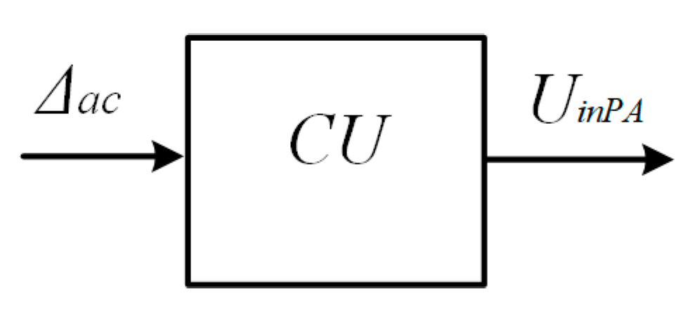
A power amplifier (PA) is a device that uses a pulse mode of the operation of semiconductor elements, since only such a mode provides effective regulation in electric drives (Figure 3).

In addition to low losses in power impulse elements, it should be noted that it is possible to control both the pulse duration τ and the repetition period T—in functions of the input signal Uin, as follows from Formula (2). It is the pulse repetition period T that most significantly affects the stability of electric drives. In modern semiconductor amplifiers and converters, the period is quite small—from 0.1 to 1 mS. However, it cannot be completely ignored.

$$\tau =f_1\left(U_{in}\right);T=f_2\left(U_{in}\right); W_{PA}=W\left(p,\tau ,T\right)$$

(2)

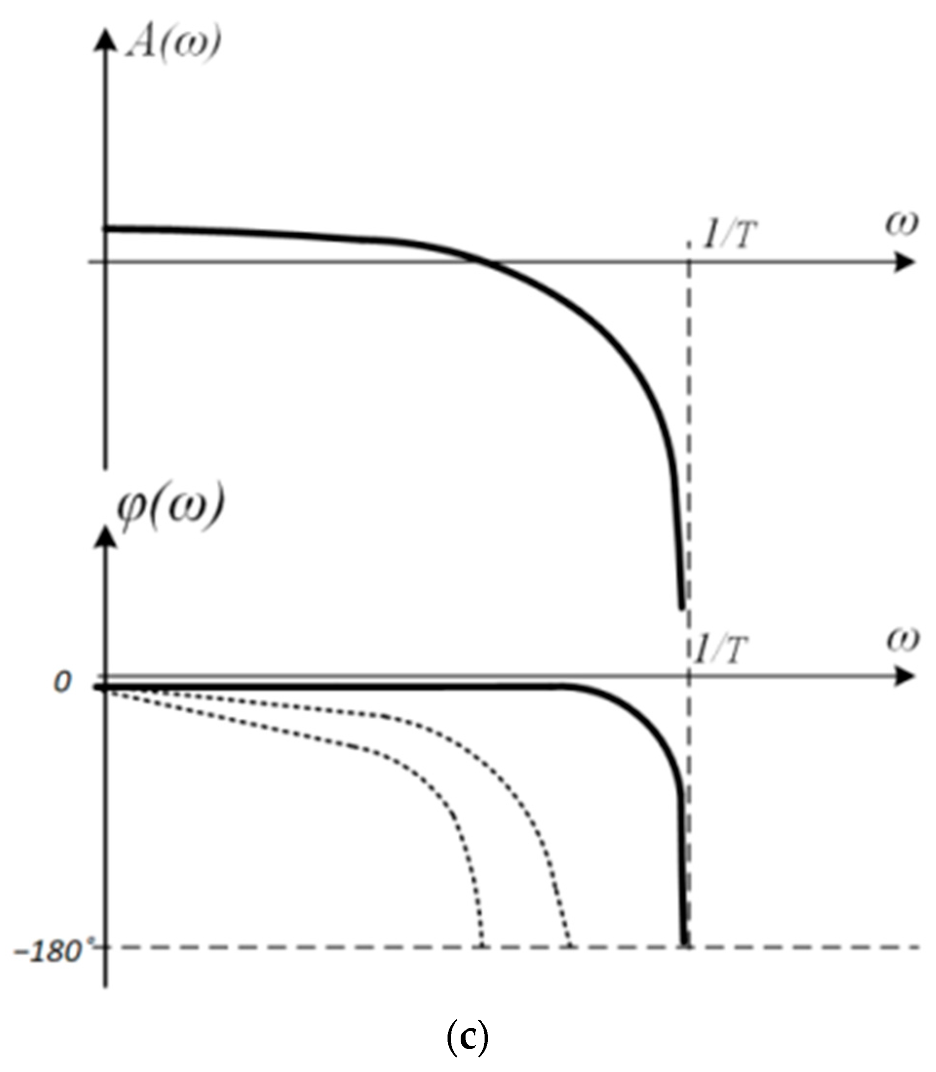
A technique [6,7] for constructing the frequency response of impulse links as suppression links is proposed (Figure 3c). However, the variable frequencies and duty cycles of the pulses make these links “even more” nonlinear, since it is the “suppression frequency” that changes.

In electric motors, the torque (T) is formed by a nonlinear function of the product of magnetic fluxes $\Phi$ (the flux created by the currents in pole windings I_ext and the flux created by the rotor current Ir), and, only in the constant-current engine (DC Motor) with an independent excitation, the moment is close to the value proportional to the magnitude rotor current Ir (3).

$$T=K\times \Phi \left(I_r,I_{exc},\mathrm{t}\right)\times I_r\approx K_1\times I_r$$

(3)

$$W_T=W\left(p,\Phi \right)\approx W_4\left(p\right)$$

Here, W₄—the transfer function of the DC motor.

In widely used induction motors, even the static torque is an essentially nonlinear function of the relative slip.

$$T\approx \frac{2M_c}{\frac{S}{S_c}+\frac{S_c}{S}}; W_T=W_5\left(p,S\right),$$

(4)

where Mc—critical torque; Sc and S—critical and current slip; and W₅—the transfer function of the asynchronous electric motor.

In the analysis of processes with maximum effort, these nonlinearities manifest themselves very significantly.

The mechanical elements of the motor, transmission and mechanism cannot be described with any accuracy by a linear equation, the mechanical links (gearbox) have nonlinear resistances T_R1 and T_R2, finite stiffnesses C and mechanical clearances λ, which, among other things, can vary depending on the speed of movement and the applied efforts (Figure 4).

$$W_{GB-WM}=W_6\left(p,K_c,T_{RM},J_{IM},J_{WM},\lambda \right)$$

Such parameters as the viscous friction coefficient Kc and the peak value of the moment of resistance T_R are very difficult to determine accurately and easily change from a variety of factors: equipment wear during long-term operation or changes in ambient temperature. The influence of these features of mechanics on processes in electric drives is exceptionally great.

It is impossible to combine all these descriptions into one structure without significant simplifications. To neglect them means to work only at speeds and power characteristics that are far from the maximum.

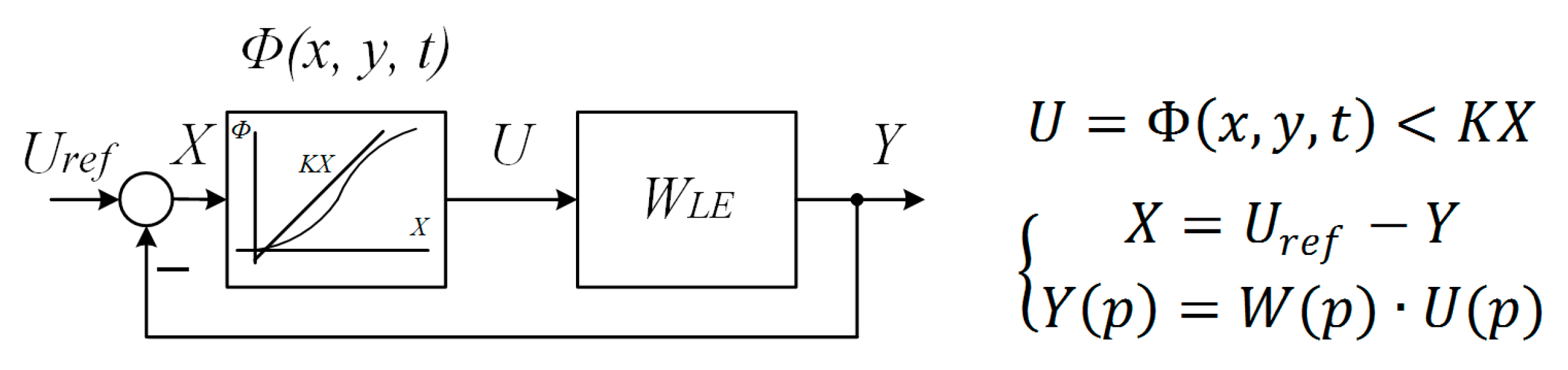
These simplifications even make the solution of the main ACT problem: the assessment of the stability of electric drive processes, to be inaccurate. Classical methods for analyzing the stability of nonlinear automatic control systems (V.M. Popov’s criterion) require reducing the initial system to the form shown in Figure 5 [8].

It is often not possible to single out one linear link and one “specific” one in an electric drive: a static nonlinearity, an impulse or a nonstationary link in order to make a real electromechanical system closer to the classical stability criteria. The methods associated with exact functional transformations, for example, the methods of the theory of systems with variable parameters, in particular, the Volterra kernel method [9,10], are very cumbersome and inefficient in engineering calculations.

We have to look for approximate solutions, which are referred to as “engineering”. At the same time, these solutions should take into account the main nonlinearities of electromechanical complexes and find effective solutions to control problems.

The most widely used engineering method is harmonic linearization, in which nonlinear links of different physical “content” are interpreted by dynamic links with amplitude and phase frequency characteristics close to linear.

In engineering calculations, the frequency Nyquist criterion is more often used [1,2,3], and the main difference of which from the criterion of V. M. Popov is that this criterion extends the requirements for frequency characteristics only to the region of frequencies that determine the dynamics of the system (the so-called “cutoff frequency”). This can have a significant impact on the correction of nonlinear electromechanical systems.

2. Nonlinear Transfer Functions and Families of Frequency Characteristics of Induction Motors

In a number of papers [11,12] on asynchronous electric drives, it is proposed to use nonlinear transfer functions and their corresponding families of frequency characteristics for electric drive analysis and correction selection. As a result of simplifying transformations, the original nonlinear structure is identified by a link with the Laplace transfer function, the parameters of which depend on the variable coordinates of the system.

$$W\left(p\right)=\frac{2M_c\left(T_2^{\prime }p+1\right)S_c}{{\omega }_1[{\left(1+T_2^{\prime }p\right)}^2{S}_c^2+{\beta }^2]},$$

(5)

Here, T′₂—rotor circuit time constant (s); Sc—critical slip; β—relative slip; and Mc—motor’s critical torque.

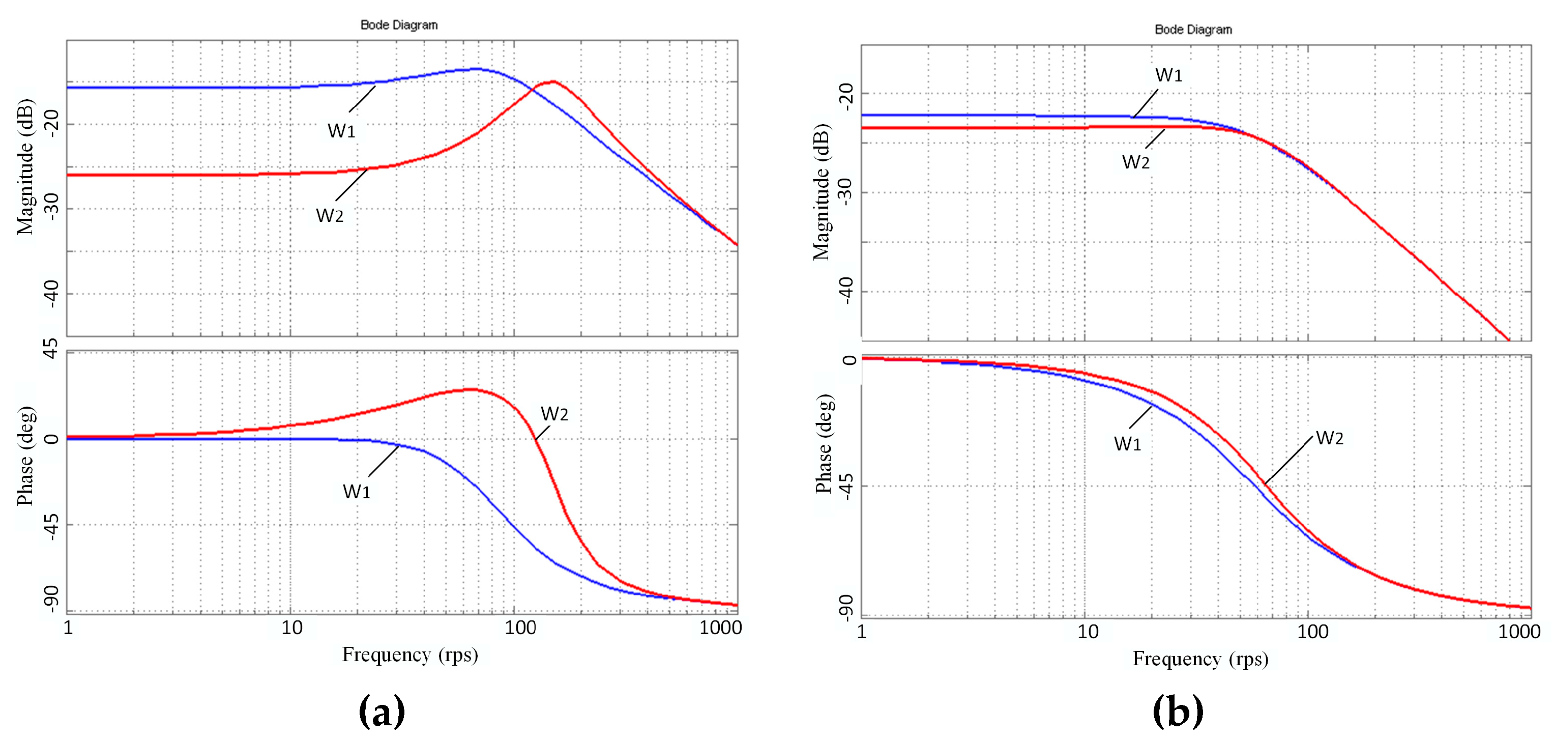
These nonlinear transfer functions correspond to families of nonlinear frequency responses. Figure 6 shows the families that depend on slip, at a constant frequency of the stator voltage (a), and on the frequency of the stator voltage at a constant slip (b).

The use of such an interpretation of complex dynamic elements makes it possible to conduct a qualitative analysis of processes in control systems of asynchronous electric drives.

It can be assumed that such an approach would be appropriate for other nonlinear electromechanical systems. In this case, variable coefficients will reflect the nonlinear properties of dynamic links more accurately than a number of other methods.

In addition, engineering stability criteria for both linear and nonlinear systems are frequency criteria (Nyquist, Mikhailov, V.M. Popov, etc.); therefore, for nonlinear electromechanical systems, it is advisable to improve methods of frequency analysis.

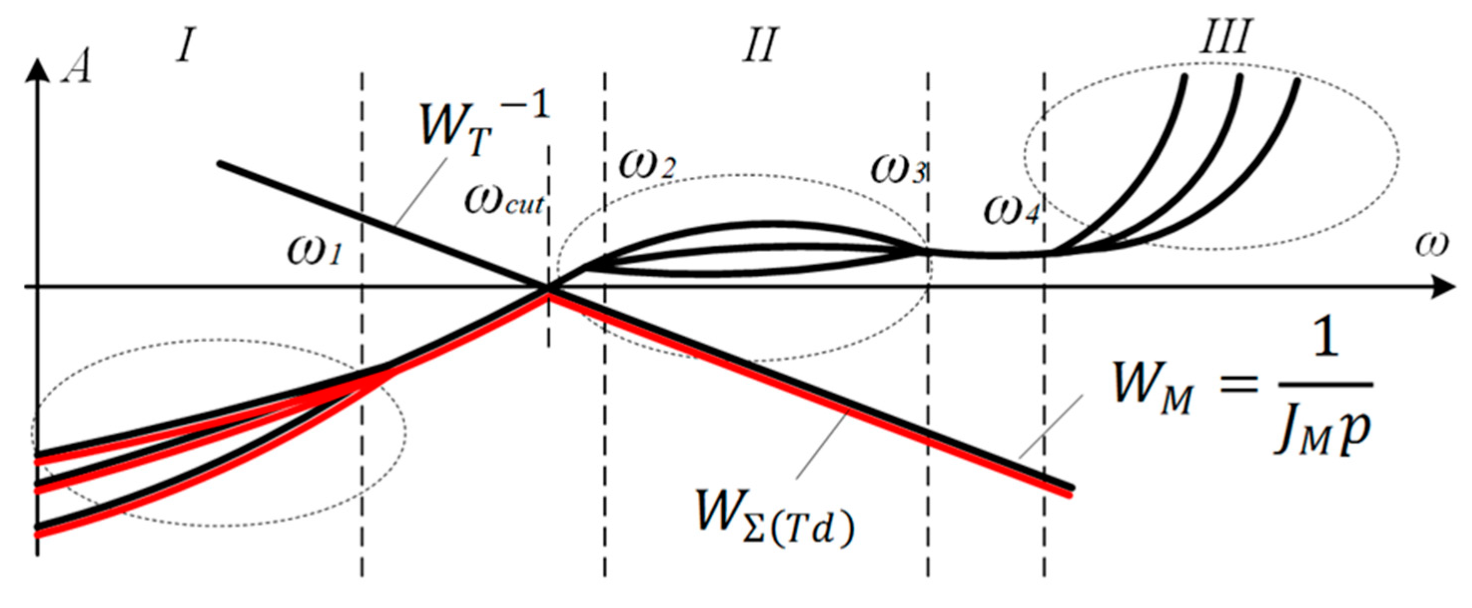
3. Families of Frequency Characteristics of a Nonlinear Electromechanical Systems and Ranges of Nonlinear Variations in Frequency Characteristics

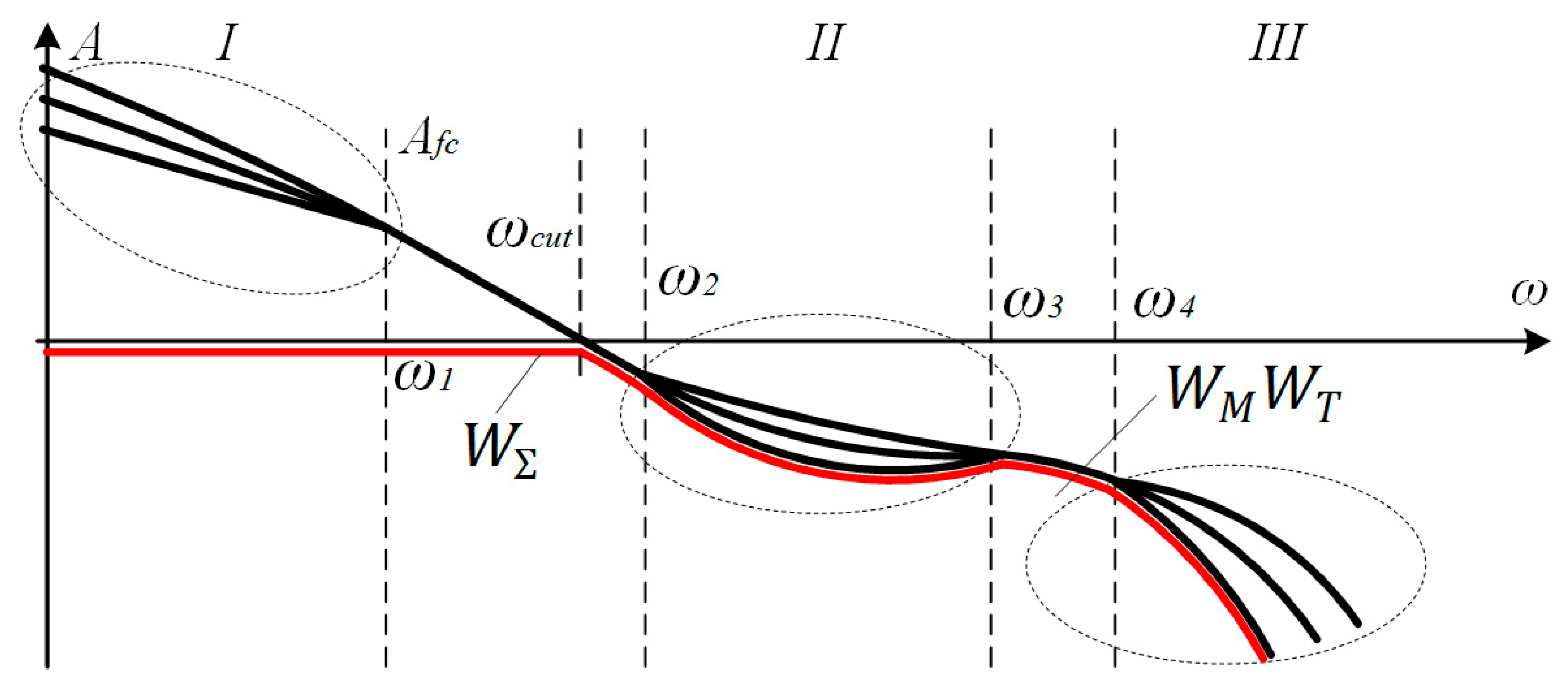
The initial block diagram of the electromechanical complex can be interpreted by the family of equivalent frequency characteristics shown in Figure 7.

The final transfer function is obtained by multiplying the transfer functions, and the logarithmic frequency response is obtained by adding:

$$W_{ED}\left(p\right)=W_{CU}\times W_{PA}\times W_T\times W_M\times W_{WN}$$

The physical meaning of the characteristic and parameter variations in three frequency ranges is as follows.

Variations in the region of low frequencies (0–ω₁) (I) are caused by the use of various controllers, including nonlinear links W₁ or W₂.

Between frequencies (ω₁–ω₂), the frequency characteristics of electric drives are close to the characteristics of linear links.

In the region of medium frequencies (ω₂–ω₃) (II), a significant role is played by nonlinear links in mechanics such as backlash and nonrigidity of the gearbox, as well as the nonlinear laws of the formation of torque in the electric motor (links W₄ or W₅ and W₆).

In the region of high frequencies (above ω₄) (III), the influence of the impulse links of the voltage converter and the discreteness of operations in the regulator (W₃) become significant.

All these areas of nonlinearity in the frequency response of the electromechanical system can be taken into account by variable terms in the formula for the final transfer function of an open-loop nonlinear electromechanical system (W_ED):

Given the formulas that define the functions $W_{CU},W_{PA},W_T, W_M and W_{WN}$, the transfer function W_ED will take the form:

$$W_{ED}=\left(\begin{array}{c}{W}_1\left(\mathsf{\Delta }, p\right)\\ W_2\left(\mathsf{\Delta }, p\right)\end{array}\right)\times W_3\left(p, \tau ,T\right)\times \left(\begin{array}{c}{W}_4\left(p\right)\\ W_5\left(p,S\right)\end{array}\right)\times W_6\left(p,K_c,T_{RM},\lambda \right),$$

(6)

Here, W_ED—the transfer function of the electric drive, its linear and nonlinear areas.

The form of the transfer function shows that the stability and efficiency of electric drives will be determined by the frequency characteristics in each of these frequency ranges, as follows from the criterion of V.M. Popov.

4. The Concept of Hyperdynamics

From the mathematics point of view, the transfer function in Laplace transforms with the parameters depending on frequency and slip is the same inexact mathematical expression as the vector equation with variable frequency signals for asynchronous electric drives. However, the continuity of the nonlinear transfer function is much closer to harmonic linearization as an “engineering” method.

The analysis of control systems using nonlinear transfer functions is “ideologically” close to the theory of the hyperstability of nonlinear systems, since this theory also considers systems with dynamic nonlinear links.

Works [11,12,13] come up with a variant of the Popov criterion for hyperstable systems described by a family of frequency characteristics. The criterion is “stated” in logarithmic frequency characteristics convenient for engineers and allowed us to justify a correction for asynchronous electric drives, which turned out to be very effective according to the results of experiments.

5. Stability of Systems with Nonlinear Dynamics

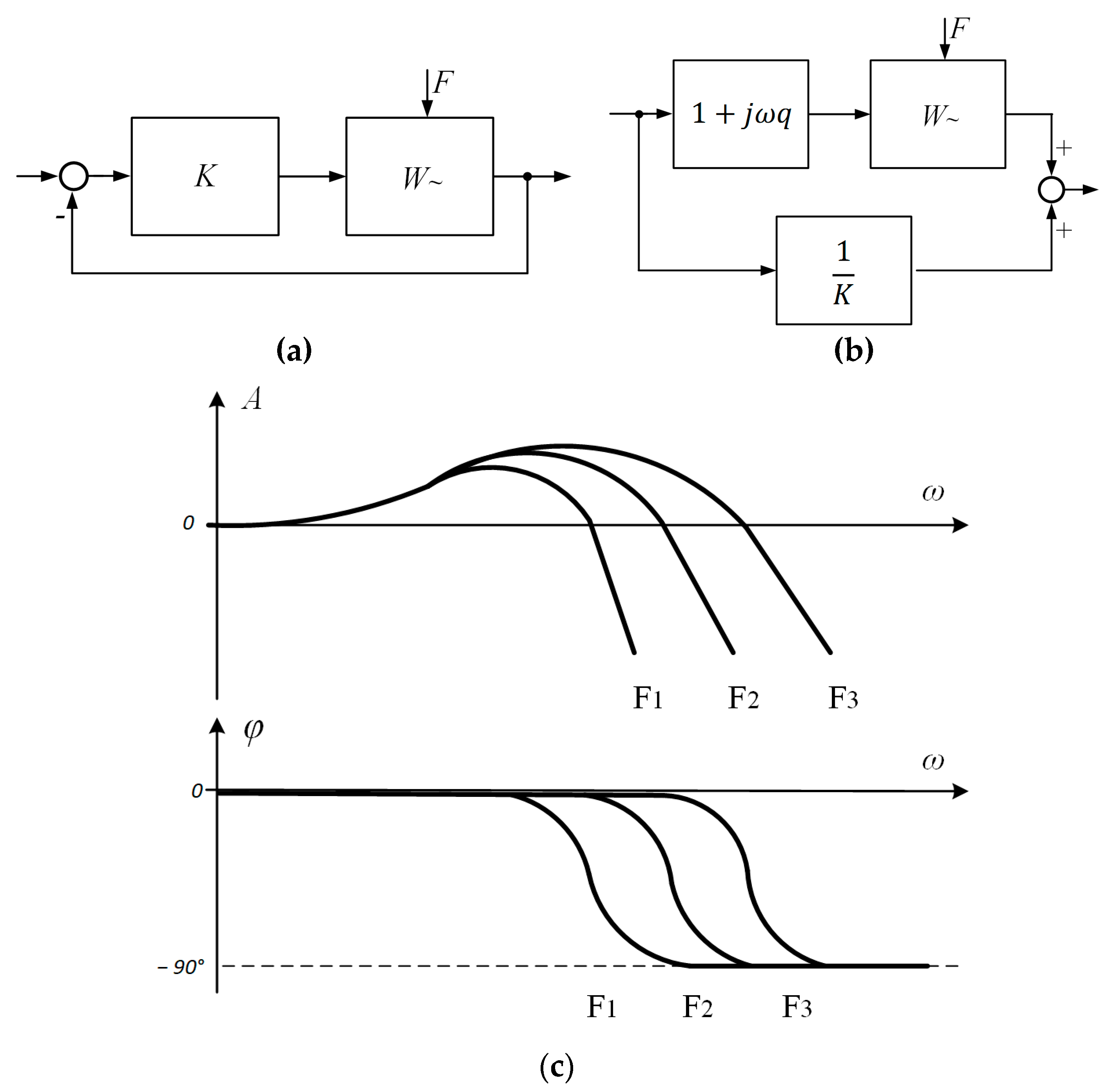
Let us assume that the original nonlinear structure can be transformed into a structure with the circuit shown in Figure 8a. Here, W_~ is a nonlinear transfer function, K is a static link limited by the coefficient K, F is an external disturbance that changes $W_{\sim }, and W_{\sim }\left(j\omega \right)$ is a family of frequency characteristics corresponding to the transfer function W_~. In order to reduce the original system to a hyperstable one, it is necessary to replace W_~ by $W_{\sim }^{*}$ in the replacement circuit, which is related to the W_~ family by the following condition: $W_{\sim }^{*}\left(j\omega \right)>W_{\sim }\left(j\omega \right)$ for all frequencies ω. Then, the hyperstability conditions can be extended to nonlinear systems of this type:

$$Re\left[\left(1+j\omega q\right)W_{\sim }^{*}\left(j\omega \right)+\frac{1}{K}\right]>0,$$

or for a system with nonlinear characteristics:

$$\phi \left[\left(1+j\omega q\right)W_{\sim }^{*}\left(j\omega \right)+\frac{1}{K}\right]>-90°$$

(7)

Condition (7) is satisfied for all characteristics of the $W_{\sim }\left(j\omega \right)$ family. The criterion imposes conditions on all frequency characteristics of a nonlinear “family” and reduces this class of nonlinear systems to the class of hyperstable systems. From this condition, it follows that for the stability of the electric drive, it is necessary to select the links of the engine and the mechanical part with certain frequency characteristics or correct them.

By analogy with hyperstable systems, systems in which transfer functions or frequency characteristics change during transient processes can be called hyperdynamic systems.

As follows from the criteria of the absolute stability and hyperstability of nonlinear systems [1,8,12], certain conditions must be satisfied by nonlinear identifiable blocks. At the same time, what is important is not the nature and rate of change of these characteristics, but only their limiting values. However, the fulfillment of stability conditions is not enough for the design of electromechanical systems. It is also necessary to evaluate the quality of the system, namely, the accuracy of processing the task signals and parrying external disturbances.

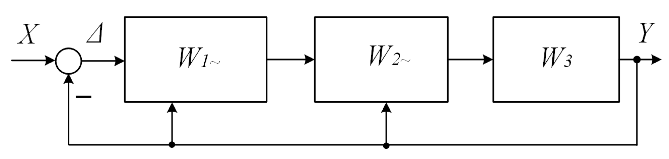
6. Cascade and Local Compensations

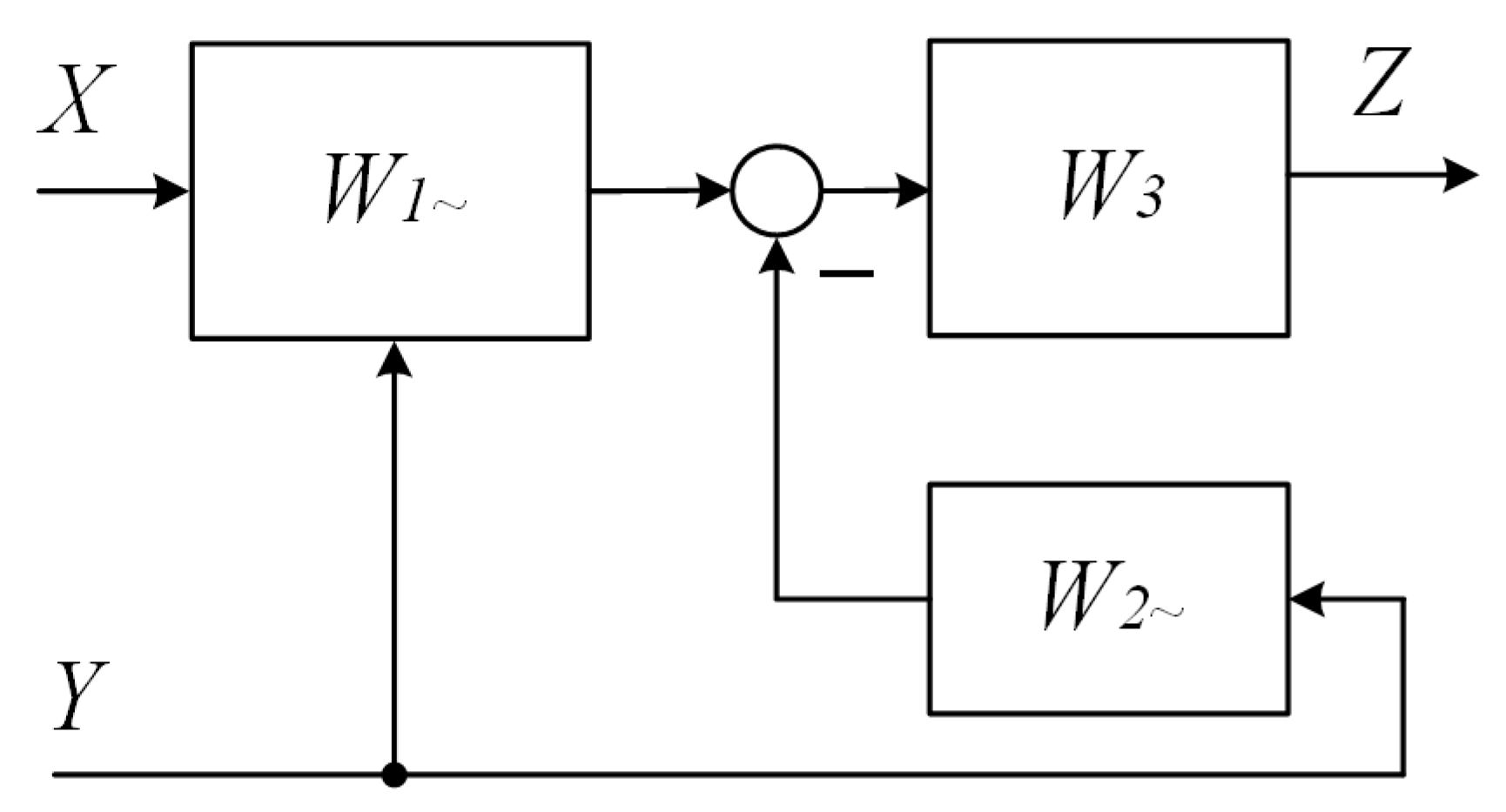
Suppose a system with a nonlinear block W_1~ corresponds to the scheme shown in Figure 9. It is possible to radically solve the problem of nonlinearities in such an ACS by adjusting W_1~ so that the resulting ($W_{1\sim }\mathsf{\Delta }{W}_{2\sim }^{*}$) ceases to depend on the changing Y coordinates. Cascade compensation shown in Figure 9 is used more often than others.

In the series with the nonlinear block, another nonlinear block W2~ is introduced such that the output signal from the combination of blocks does not depend on Y. However, in real systems, the complete compensation of nonlinearities is impossible, and the correction block transfer function, except for the exact block $W_{2\sim }^{*}$, will contain an error ΔW₂.

The causes of errors in the correction block are diverse: from natural errors in measuring signals to inaccuracies in models and the fundamental error in the operation of multiplying nonlinear operators.

If we consider the diagram in Figure 9 and represent the product of two operators, taking into account the error, then the equation will take the form:

$$\begin{array}{c}{X}_2=\mathsf{\Delta }\times W_{1\sim }\times W_{2\sim }=\mathsf{\Delta }\times W_{1\sim }\left(W_{2\sim }^{*}+\mathsf{\Delta }{W}_2\right)=\mathsf{\Delta }\times \left(W_{1\sim }\times W_{2\sim }^{*}+\mathsf{\Delta }\times W_2\times W_{1\sim }\right)=\\ =\mathsf{\Delta }\times W_{1\sim }\times W_{2\sim }^{*}+\mathsf{\Delta }\times W_2\times W_{1\sim }\end{array}$$

(8)

The final error $\mathsf{\Delta }{W}_2\times W_{1\sim }$ will be determined not only by the error itself but also by the original transfer function $W_{1\sim }$, that is, it will act in the entire frequency range and affect processes, including their stability, very significantly.

Another option is to use local links according to the ACS output coordinates (Figure 10).

In this case, the formula will take the form:

$$W_{1\sim }+W_{2\sim }=W_{1\sim }+\left(W_{2\sim }^{*}+\mathsf{\Delta }W\right)=(W_{1\sim }+W_{2\sim }^{*})+\mathsf{\Delta }W=W\left(j\omega \right)+\mathsf{\Delta }W,$$

(9)

In this case, W(jω) does not depend on Y.

The dynamic error ΔW will “work” in a much smaller frequency range, since there is no term connecting the error and the original transfer function, as in the formula. Thus, the effect of the error on the operation of the entire nonlinear system will be significantly weakened.

In studies of the dynamics of asynchronous electric drives [13,14], the effectiveness of positive dynamic coupling by the active component of the stator current—an analogue of link in respect to moment—is shown. An electric drive with this connection turned out to be much more accurate and dynamic than a well-studied drive with vector control, which is a sequential correction that linearizes the influence of the stator voltage frequency on the drive.

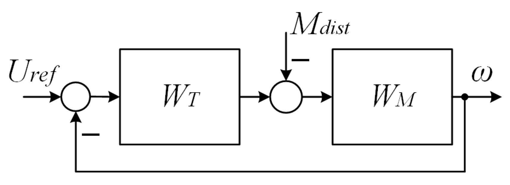
7. Parrying External Disturbances

To solve the problems of a large number of technological units, electric drives (the block diagram of which is shown in Figure 11) must, as a rule, solve TWO TASKS.

• The tracking of the reference signals provides the required changes in the output coordinates of electromechanical systems, most often the rotation speed ω to the given signal Uref.

  Figure 11. Electromechanical system with reference input (Uref) and disturbance input (Mdist).

  Figure 11. Electromechanical system with reference input (Uref) and disturbance input (Mdist).

Nonlinearities in the frequency response of a closed loop with respect to the signal Uref have little effect on the final frequency response and processes. This follows from the LFC of the closed circuit. Frequency response variations affect only the loop stability margins (in the cutoff-frequency range) and the static control error (in the low-frequency range).

As mentioned above, the stability of the electric drive is mainly determined by the combination of the frequency characteristics of the mechanical part and the formation of the moment in the electric motor. If the variability and oscillation of these links are located in close frequency ranges, it is very difficult to stabilize such an electric drive, as follows from the frequency characteristics shown in Figure 12. Elements should be selected according to well-known methods, or a correction should be selected especially accurately. Moreover, consistently, as follows from the formulas, it is not very effective.

If we consider stability according to the Nyquist criterion, then we must first of all pay attention to the frequencies of the range ω₂–ω₃. Then, according to the criterion of V.M. Popov, it is necessary to evaluate the entire frequency range (0–ω₄). In this case, one can “see” the influence on the stability of the pulsed nature of the power amplifier (PA) link.

2.

The mode of parrying the disturbing factors.

As a result of the control loop operation, their influence on the processes of changing the controlled coordinate should be minimal.

Figure 13 shows the AFC of the system with respect to the disturbing input Mdist. The nonlinearities of the frequency characteristics at low frequencies directly determine the value of the change in the controlled coordinate from the disturbing. The overall stability conditions remain similar, although it should be taken into account that the operation of frequency response inversion for nonlinear structures can lead to other frequency responses than in Figure 13.

The transfer functions of the control system for this input are given below for a system with sequential correction:

$$\begin{array}{c}{W}_{\mathsf{\Sigma }\left(Td\right)}=\frac{W_M}{1+W_M\times W_T\times W_K}=\frac{W_1}{1+W_M\times W_T\times \left(W_K^{*}+\mathsf{\Delta }W\right)}=\\ =\frac{W_1}{1+W_M\times W_T\times W_K^{*}+\mathsf{\Delta }W\times W_M\times W_T}=\frac{1}{1+W_{\mathsf{\Sigma }L}+\mathsf{\Delta }W\times W_M\times W_T};\end{array}$$

(10)

With local correction, the transfer function (10) takes the form:

$$W_{\mathsf{\Sigma }\left(Td\right)}=\frac{W_M}{1+W_M\times W_T+W_K}=\frac{W_M}{1+W_M\times W_T\times W_K^{*}+\mathsf{\Delta }W}=\frac{1}{1+W_{\mathsf{\Sigma }L}+\mathsf{\Delta }W}$$

(11)

As follows from the formulas, local correction does not increase its errors due to interaction with the structures of the electric drive, which gives such corrections a certain advantage in real systems; in this case, the “work” of local correction is not associated with unpredictable nonlinear operations with frequency characteristics.

8. Experimental Studies, Their Connection with Representation and Mutual Complementation

For electric drives in which nonlinearities cannot be neglected, experiments play an exceptional role, which is determined by a number of conditions.

First, their results should confirm the validity of the proposed management principles, since theoretically it is most often impossible to prove this.

Secondly, it is important to show that the results of the experiment apply to a certain area of external disturbances and driving signals—which is, to other modes of operation, of interest to mechanisms in which electric drives operate.

Third, experiments must be reproduced under similar conditions in order to find confirmation of their results.

From these positions, the identification of a nonlinear electric drive by continuous nonlinear transfer functions is more logical than, for example, vector equations, which theoretically cannot form a “continuous” space of system states. To such nonlinear systems, the stability theorems of V.M. Popov [8], which become the theoretical basis for the mutual complement of experiments and the identification method, can be applied. The theory of hyperstability operates with the boundary characteristics of nonlinear objects. This approach is very effective for engineering analysis, and it is the continuous identification of nonlinear structures that is more justified for the analysis of dynamics problems in general. The same theorem can become a rationale for the effectiveness of local corrections, which turned out to be more accurate for the considered operating modes than traditional methods for interpreting and correcting the frequency regulation of asynchronous electric motors.

The bench tests of asynchronous electric drives as essentially nonlinear structures, as well as the modeling of their dynamic modes, the results of which are given in [11,12,13,14], showed that the corrections chosen for a nonlinear control system, for a system with a nonlinear frequency response (DPF), turned out to be much more effective traditional corrections of asynchronous electric drives—vector and scalar, built on the principles of sequential correction. These differences are especially significant for the modes of parrying stepped and periodic surges of loads [11,14], in which the frequency characteristics of all dynamic links play an important role in a wide frequency range.

9. Conclusions

• Electromechanical devices and electric drives operating with maximum speed, accuracy and effort from the point of view of automatic control theory are nonlinear, nonstationary structures with different natures. It is possible to neglect any of the main nonlinearities of electromechanical devices in their design only to the detriment of their most important characteristics.
• The most appropriate engineering method for the analysis and synthesis of control systems for nonlinear electromechanics is the use of nonlinear transfer functions and families of frequency characteristics that take into account all the main nonlinearities of electromechanics: nonlinear laws of regulation, nonlinearities in the formation of torque, finite stiffness and backlash of the mechanical links of systems and the impulsive nature of modern power amplifiers. In this case, the nonlinear dynamics of all these links is of particular importance.
• The proposed method for assessing the stability and efficiency of nonlinear electromechanical systems, which allows for taking into account nonlinear dynamics according to criteria arising from the theories of absolute stability and hyperstability of V.M. Popov, is confirmed by experimental studies with such essentially nonlinear systems as asynchronous electric drives with frequency control.
• From the analysis of processes according to the proposed method and previous experiments, it follows that the correction of nonlinearities by local connections is more effective than the sequential one, although it is the sequential one that is most widely used in modern automatic control systems.