Abstract
The current investigations are carried out to study the influence of the Darcy–Forchheimer relation on third-grade fluid flow and heat transfer over an angled exponentially stretching sheet embedded in a porous medium. In the current study, the applied magnetic field, Joule heating, thermaldiffusion, viscous dissipation, and diffusion-thermo effects are incorporated. The proposed model in terms of partial differential equations is transformed into ordinary differential equations using suitable similarity transformation. The reduced model is then solved numerically with the help of MATLAB built-in function bvp4c.The numerical solutions for velocity profile, temperature profile, and mass concentration under the effects of pertinent parameters involved in the model are determined and portrayed in graphical form. The graphical effects of the skin friction coefficient, the Nusselt number, and the Sherwood number are also shown. From the displayed results, we conclude that when the Joule heating parameter is enlarged, the velocity and the temperature of the fluid are increased. We observed that while enhancing the viscous dissipation parameter (Eckert number) the fluid’s velocity and temperature increase but decreases the mass concentration. By increasing the values of the thermal-diffusion parameter, the velocity distribution, the temperature field, and the mass concentration increase. When the diffusion–thermo parameter rises, the velocity field and the temperature distribution increase, and the reverse scenario is seen in the mass concentration. The results of the current study are compared with already published results, and a good agreement is noted to validate the current study.
1. Introduction
Non-Newton fluid flow is widely used in many technological and industrial systems. Non-Newtonian liquids have been widely approved by researchers due to their great technological and industrial applications, such as paper production, polymers, coal slurries, cosmetics, oil retrieval, clay mixtures, etc. The work of researchers who paid attention to third-grade fluid flow with different flow features over the different flow geometries is now being highlighted. The analytical solutions of magnetohydrodynamic third-grade fluid flow with changing viscosity were determined by Elahi et al. [1]. Muhammad et al. [2] investigated the thermal bioconvection third-grade nanofluid flow in a stagnation point over a stretching cylinder with consideration of motile organisms. Awaiset al. [3] investigated the effect of varied characteristics on heat and mass transfer in bioconvective nanofluid with gyro-tactic microorganisms under the influence of a magnetic field. In [4,5,6,7,8,9,10,11], third-grade fluid flow and heat transfer phenomena with diverse fluid features past different geometries were encountered. Sahoo [12] investigated the process of transferring heat to a third-degree liquid over a simple striped sheet with a slightly smoother texture. Pakdemirli [13] discussed in detail the flow of the third-grade liquid boundary layer. The work of Javanmard et al. [14] focused on the fully developed flow of third-degree fluid in a trench under the influence of the applied magnetic field and the changing boundary conditions. The process of transferring heat to a third-degree liquid flow in the area of the stretching sheet with the effect of a slip flow impact was investigated numerically by Sahoo and Do [15].
The preceding paragraph highlighted studies that dealt specifically withthird-grade fluid flow on diverse flow geometries. Now, the flow mechanisms over the stretching sheet, especially an exponentially stretching plate, are highlighted. Much work on stretching sheets has been documented, due to their applications in engineering and technology fields.Their applications can been seen in extrusion materials, chemical engineering plants, drawing of plastic films, annealing of copper wires, and glass fiber, etc. In [16,17,18,19,20,21,22,23], the boundary layer flow of Newtonian and non-Newtonian fluids was studied using different features across an exponentially stretching sheet. Kumar et al. [24] used Soret, Dufour, Joule temperature, chemical reactions, magnetic field, and slip effects to test heat and mass transfer to angled sheets fixed in a porous media. Magyari and Keller [25] investigated heat and mass transport in boundary layer flow across an exponentially stretching sheet.
The current paragraph is concerned with studies focusing on the Joule heating effects on flow phenomena. The technique of producing heat by passing an electric current via a conductor is known as Joule heating, also known as resistive, resistance, or Ohmic heating. Jouleheating, also known as resistive heating, is employed in a variety of electronics and industrial processes. A heating element is a component that transforms electricity into heat. Joule heating may be used frequently in food processing equipment. Heat is released inside the meal when a current is passed through the food substance (which acts as an electrical resistor). Heat is generated by the alternating electrical current combined with the resistance of the food. The combined effects of Joule heating, viscous dissipation, thermal radiation, and heat generation on a magneto-hydrodynamic were analyzed by Ur Rasheed [26]. Swain et al. [27] discussed the Joule heating and viscous dissipation effects on magnetohydrodynamic flow and heat transfer over a stretchable surface embedded in a porous medium. Zeshan et al. [28] investigated the numerical study of magnetohydrodynamic nanofluid flow over a wavy surface in the presence of thermal radiation, viscous dissipation, and Joule heating effects using the Keller Box method. The process of heat and mass transfer in the blood flow in the presence of magnetic field effects, Joule heating effects, and Hall effects has been explored by Bhatti et al. [29]. Shamshuddin et al. [30] studiedthe combined effects of viscous dissipation and Joule heating in Fourier MHD squeezing flow over the raga plate in the presence of thermal radiation. The magnetohydrodynamic micropolar fluid flow and heat transfer phenomena under the effects of Joule heating and viscous dissipation effects were studied by Haque et al. [31].
The research community has devoted much studyto the magneto-hydrodynamics flow with different fluid characteristics. The study of the effects of magnetic fields has important applications in physics, chemistry, and engineering. Much engineering equipment, such as the producer of magnetohydrodynamic (MHD), pumps, bearings, and boundary layer process, is affected by contact between the electrically conducting fluid and the magnetic field. Due to various applications, in geophysics, magnetohydrodynamic power generation, and so on, an enormous amount of research on the different fluid features along several geometries with diverse flow conditions has been published. On the surface of stretchable cylinder, MHD Casson flow is proposed by Tamoor et al. [32]. Magnetohydrodynamic chemically reacting fluid flow past an exponentially stretched surface was studied by Pattnaik et al. [33]. Radiative magenohydrodynamic flow past an exponentially stretched plate was evaluated numerically by the Homotopy Analysis Method in [34]. Salahuddin et al. [35] shed light on the topic of MHD Williamson fluid flow under the influence of generalized heat transfer laws pasta stretchable surface with variable thickness. Kumar et al. [36] revealed the process of MHD flow by analyzing the heat source and sink impact. Studies about magnetohydrodynamic flow past diverse shapes have been encountered in [37,38].
In the paragraphsabove, studies of the third-grade fluid flow process on stretching sheets with Joule heating effects, thermaldiffusion and diffusion-thermo effects on boundary layer flow of Newtonian and non-Newtonian fluids and the magneto-hydrodynamics flow in the different media were highlighted. Much work on porous medium has been accomplished in the existing literature due to its enormous application in various fields of sciences. The flow of porous media has been an attraction of the research for the past decades. The study of fluid flow and heat within permeable media is also very important in many other fields of science and engineering, such as biomedical and biomedical studies. Khan et al. [39] gave ananalysis of thin-film flow of second-grade fluid flow over a stretching sheet fixed in a porous medium. Ali et al. [40] proposed a study on magnetohydrodynamic flow of viscoelastic fluid over a stretching sheet surrounded by a porous medium with the effects of slip flow. A numerical evaluation of unsteady hydromagnetic fluid flow over a slippery stretching sheet fixed in a porous medium in the presence of thermal radiation was performed by Makinde et al. [41]. The different fluid flows and heat transfer phenomena in a porous medium were discussed in [42,43,44,45,46]. Ali et al. [47] studied the phenomenon of unsteady magnetohydrodynamic Falkner–Skan wedge flow of non-Newtonian nanofluid under the effect of thermal radiation and activation energy. Magnetodhyrodyanmic bioconvection nanofluid flow with melting effect on generalized heat transfer laws along the leading edge has beentackled numerically by using finite element method in Ref. [48]. The combined effects of magnetic field and thermal radiation, nanoparticles diameter, and Darcy–Forchheimer flow along the cylinder was considered by Ali et al. [49].
In the existing literature, many studies have been conducted on non-Newtonian fluids due to practical applications in industry and engineering, such as food processing, lubrication processes, and paper-making processes. In the present paper, a numerical study on heat and mass transfer via third-grade fluid with the Darcy–Forchheimer relation effects past inclined exponentially stretching sheet embedded in a porous medium has been performed. Furthermore, thermal-diffusion, applied magnetic field, diffusion-thermo effect, viscous dissipation, and Joule heating effects have been incorporated. A formulation of the problem is given in Section 2. The entire solution procedure is presented in Section 3. The obtained results are portrayed and discussed in Section 4, and at the end, the whole research work is concluded.
2. Formulation of the Problem
Consider the steady flow and the incompressible, viscous, and two-dimensional flow of an electrically conducting third-grade fluid over an inclined and exponentially stretching sheet embedded in the porous medium. A uniform applied magnetic field is found in the y-direction to the fluid system. The Darcy–Forchheimer relation is considered in the model. The Joule heating, viscous dissipation, thermal-diffusion, and diffusion-thermo effects are taken in the flow model. The sheet is heated and has the temperature with and the concentration at the surface is with the condition . The x-axis is taken in the direction of the flow, and the -axis is taken as normal to the direction of the flow. The velocity components are in the direction of , respectively. The flow configuration of the coordinate system is shown in Figure 1. As the flow is driven under the consideration of the applied magnetic field, the leading term in the Lorentz force (per unit volume) participating in the equation of motion is defined as
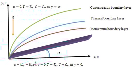
Figure 1.
Flow configuration and coordinate system.
Maxwell equation state.
By Ohm’s law
where is the velocity vector, is the density, is the current density, B is the total magnetic field, is the magnetic permeability, is the electric field, and is the electrical conductivity.
The Reynolds number is so small that the flow is laminar. Hence
For third-grade fluid, a Cauchy stress is given [12]:
Here, and are the material moduli. The designation is the coefficient of viscosity. In Equation (5), is the spherical stress because of the incompressibility constraint. The kinematical tensors , , and are defined by
where the notations , denote the gradient operator and the velocity vector fields, respectively. Here, the material time derivative is . If all the motions of the fluid are compatible with thermodynamics and if it is assumed that specific Helmholtz free energy is very small when the fluid is restinglocally, then
The governing relation suitable thermodynamically for third-grade fluid becomes
By following [12,24], we have the following flow equations:
The flow conditions are
Here, is the stretching velocity, is wall temperature, and is wall concentration. Here, is reference velocity, is reference temperature, and is concentration. Here, is the coefficient of inertia and is the drag coefficient, is the porous medium permeability, and are material moduli. The symbols , , and are kinematic viscosity, magnetic field strength, fluid density, and thermal-diffusion ratio, respectively. The designations , , , and , are concentration susceptibility, dynamic viscosity, thermal conductivity, and means fluid temperature, respectively. The symbols , and represent specific heat at constant pressure, thermal-diffusivity, mass-diffusivity, and electrical conductivity, respectively. The symbol is thermal expansion coefficient and is concentration expansion coefficient.
3. Method of Solution
The current section focuseson explaining the whole solution procedure for the solution of Equations (9)–(12) along with boundary conditions (13).
3.1. Similarity Formulation
The non-linear and coupled partial differential equations given in Equations (12)–(14) along with boundary conditions (15) are difficult to solve. Accordingly, these equations are first changed to ordinary differential equations with the help of similarity transformation given in [24].
After the substitution of variables given in Equation (16) into Equation (11), then it is satisfied automatically, and Equations (12)–(15) take the following form.
Boundary conditions
Here, is called the local inertial coefficient, is known asthe third-grade fluid parameter, is termed as the buoyancy ratio parameter, is called the cross-viscous parameter, = represents the Prandtl number, is known as the Eckert number, is called the Joule heating parameter, designates the diffusion-thermo parameter (Dufour number), is called the Richardson number, , designates the thermal-diffusion parameter, is the viscoelastic parameter, = is the Schmidt number, is the permeability parameter, and is called the magnetic field parameter. Here, and are the Reynolds number and Grashof number, repectively. Here, the prime symbol represents the differentiation w.r.t to similarity variable .
The mathematical expressions for the Skin friction coefficient, the Nusselt number, and Sherwood number are
where
are typical stress tensor, heat, and mass flux at surfaces, respectively. Finally, the expressions for drag force, local Nusslt, and local Sherwood are given below:
where is called the local Reynolds number.
3.2. Solution Technique
The analytical solution of Equations (15)–(18) is so difficult that numerical solutions are determined for various values of the parameters, namely local inertial coefficient , third-grade fluid parameter , buoyancy ratio parameter , cross-viscous parameter , Prandtl number , Eckert number , Joule heating parameter , diffusion-thermo parameter (Dufour number) , Richardson number , thermal-diffusion parameter(Soret number), viscoelastic parameter , Schmidt number permeability parameter , and magnetic field parameter . The numerical results of the considered model are determined with the use of MALAB built-in Numerical Solver bvp4c. The solverbvp4c is based on the finite difference code, which uses the three-stage Lobato formula, and it is known as a collocation formula. There is a -continuous solution of collocation polynomial, which is accurate upto the fourth-order in the interval of integration. There is a strong dependence of selection of mesh and control of error on continuous solution.An interval of integration is divided into subintervals by employing the mesh of points in the technique of collocation. A solver finds solutions by solving the whole set of algebraic equations, and on all subintervals, a condition of collocation is applied. For visible and asymptotic convergence of the solution, η∞ = 10.0 at infinity is taken. There is the estimation of the solver at each subinterval. Equations (17)–(19) are reduced to a set of first-order ODEs and then are substituted into algorithm of the bvp4c for solutions. We set
Boundary Conditions’
Theses equations are solved to obtainthe numerical solutions of velocity profile , temperature profile , and mass concentration . In addition, theskin friction coefficient , the Nusselt number , and the Sherwood number are computed and their graphical effects are demonstrated. In next section, the results are demonstrated in graphs, and the tabular forms are discussed in detail.
4. Results and Discussion
This section analyzes and discusses in detail the physical attributes of the unknown properties of interest under the effect of the physical parameters that appeared in flow equations and the effects of local inertial coefficient ,third-grade fluid parameter , buoyancy ratio parameter , cross-viscous parameter , Prandtl number , Eckert number , Joule heating parameter , diffusion-thermo parameter (Dufour number) , Richardson number , thermal-diffusion parameter(Soret number), viscoelastic parameter , Schmidt number permeability parameter , and magnetic field parameter on velocity field , temperature field , mass concentration . The influences of said parameters on skin friction coefficient heat transfer rate coefficient (Nusselt number) , and mass transfer rate coefficient (Sherwood number) are estimated and plotted in graphs (see Figure 2, Figure 3, Figure 4, Figure 5, Figure 6, Figure 7, Figure 8, Figure 9, Figure 10, Figure 11, Figure 12, Figure 13, Figure 14, Figure 15, Figure 16, Figure 17, Figure 18, Figure 19, Figure 20, Figure 21, Figure 22, Figure 23, Figure 24, Figure 25, Figure 26, Figure 27, Figure 28, Figure 29, Figure 30, Figure 31, Figure 32 and Figure 33) and in tabular form. The numerical results of the present study are compared with available results in the literature and are presented in Table 1.
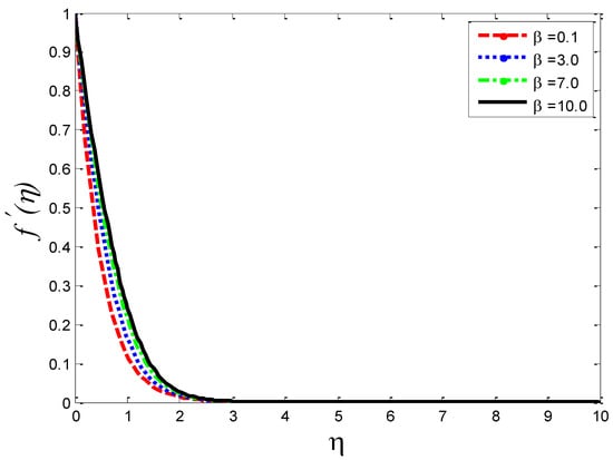
Figure 2.
Impact of third-grade fluid parameter on velocity profile .
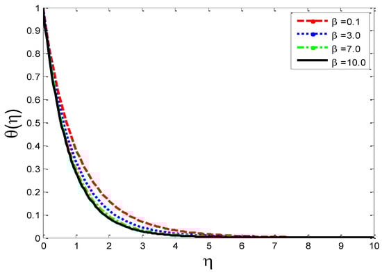
Figure 3.
Impact of third-grade fluid parameter on temperature profile .
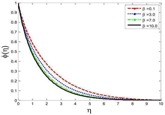
Figure 4.
Impact of third-grade fluid parameter on mass concentration .
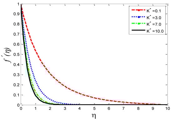
Figure 5.
Impact of permeability parameter on velocity profile .
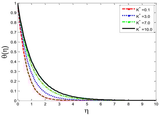
Figure 6.
Impact of permeability parameter on temperature profile .
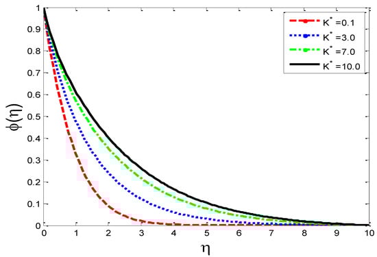
Figure 7.
Impact of permeability parameter on mass concentration .
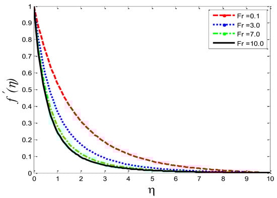
Figure 8.
Impact of local inertial coefficient on velocity profile .
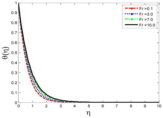
Figure 9.
Impact of local inertial coefficient on temperature profile .
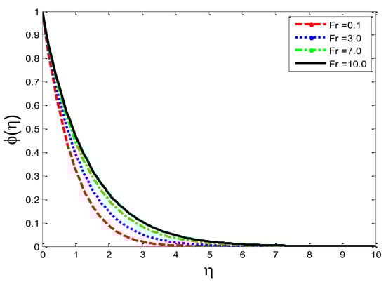
Figure 10.
Impact of local inertial coefficient on temperature profile .
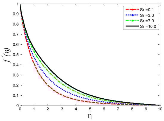
Figure 11.
Impact of thermal-diffusion parameter on velocity profile .
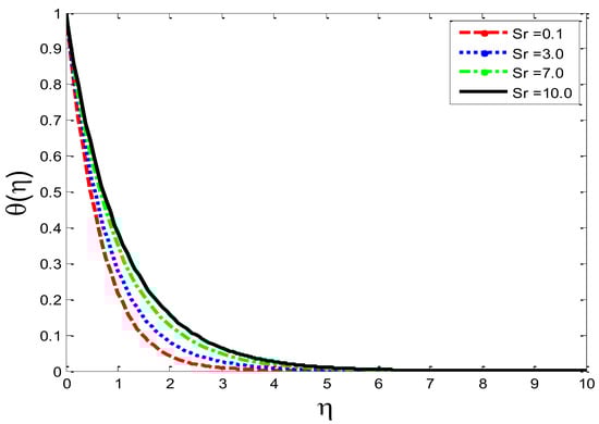
Figure 12.
Impact of thermal-diffusion parameter on temperature profile .
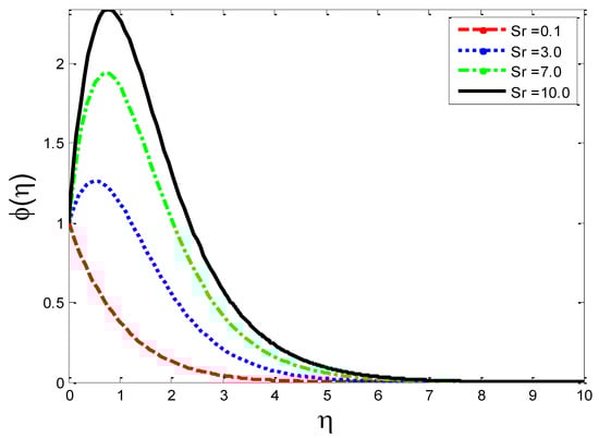
Figure 13.
Impact of thermal-diffusion parameter on mass concentration .
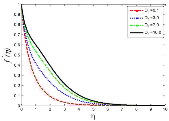
Figure 14.
Impact of diffusion-thermo parameter on velocity profile .
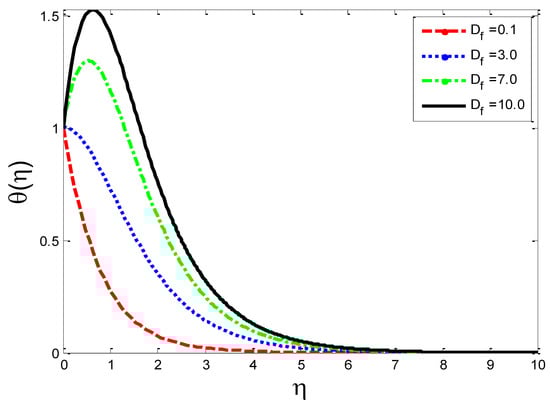
Figure 15.
Impact of diffusion-thermo parameter on temperature profile .
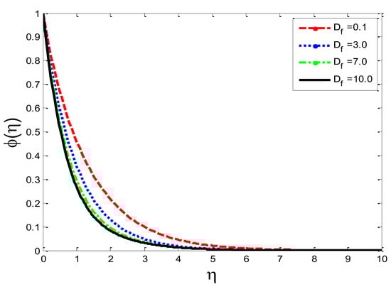
Figure 16.
Impact of diffusion-thermo parameter on mass concentration .
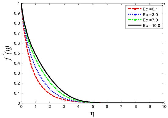
Figure 17.
Impact of Eckert number on velocity profile .
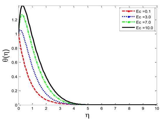
Figure 18.
Impact of Eckert number on temperature profile .
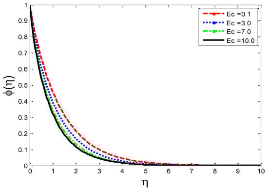
Figure 19.
Impact of Eckert number on mass concentration .
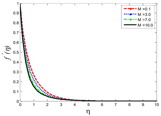
Figure 20.
Impact of magnetic field parameter on velocity profile .
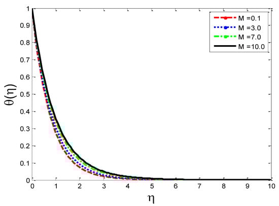
Figure 21.
Impact of magnetic field parameter on temperature profile .
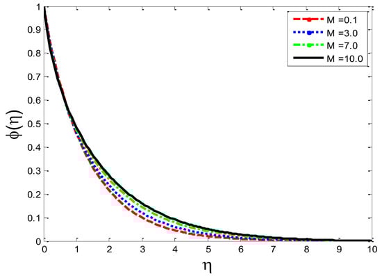
Figure 22.
Impact of magnetic field parameter on mass concentration .

Figure 23.
Impact of Joule heating parameter on velocity profile .
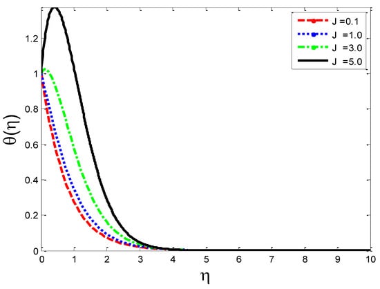
Figure 24.
Impact of Joule heating parameter on temperature profile .
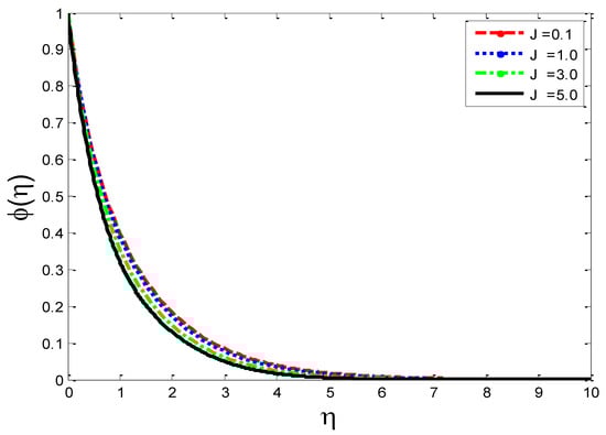
Figure 25.
Impact of Joule heating parameter on mass concentration .
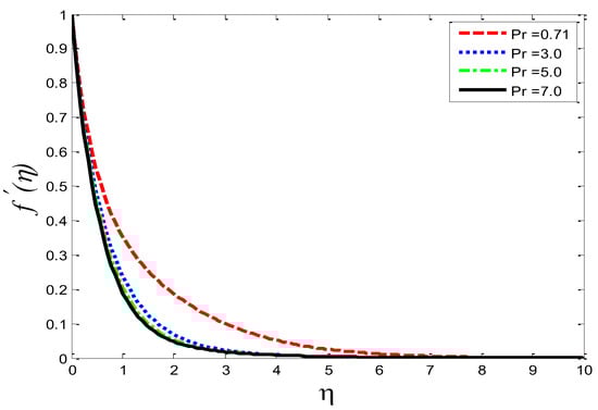
Figure 26.
Impact of Prandtl number on velocity profile .
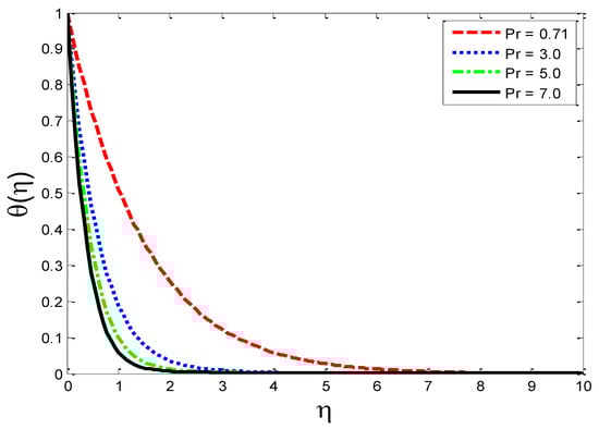
Figure 27.
Impact of Prandtl number on temperature profile .
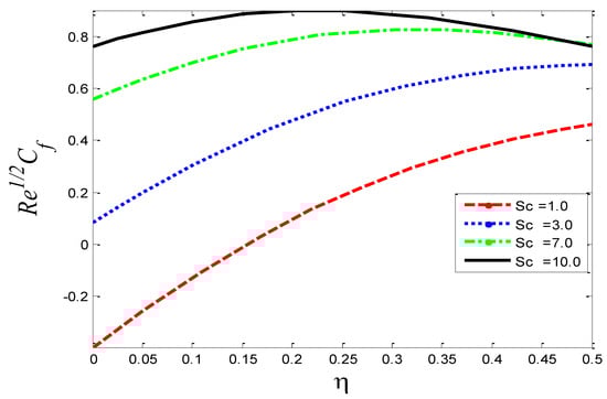
Figure 28.
Impact of Schmidt number on skin friction coefficient .

Figure 29.
Impact of the Schmidt number on the Nusselt number .
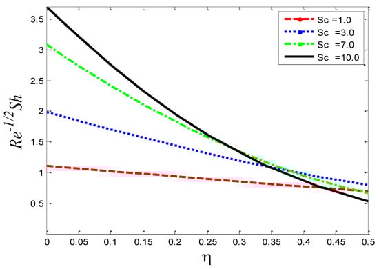
Figure 30.
Impact of Schmidt number on Sherwood number .
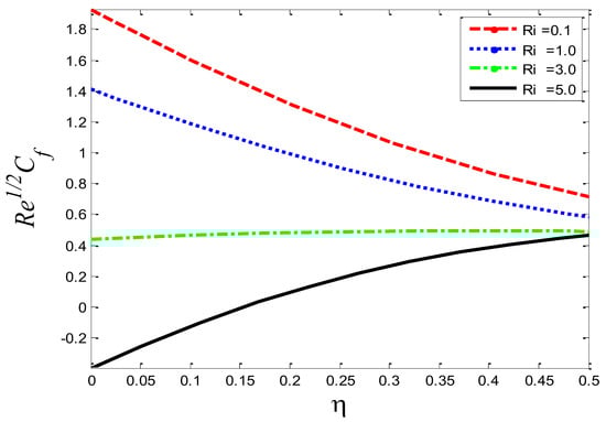
Figure 31.
Impact of Richardson number on skin friction coefficient .
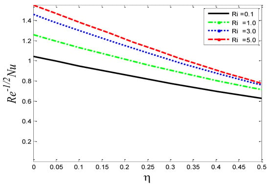
Figure 32.
Impact of the Richardson number on the Nusselt number .
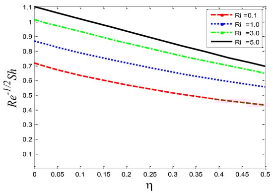
Figure 33.
Impact of the Richardson number on the Nusselt number .

Table 1.
Comparison of results for when .
4.1. Impact of Pertinent Parameters on and
The physical influence of on the velocity field , the temperature field , and the mass concentration is illustrated in Figure 2, Figure 3 and Figure 4, respectively. From the results, we see that by augmenting the numeric values of , the velocity of the fluid increases, but the opposite trend is noted in and . Physically, it is true because by increasing , the fluid’s viscosity is reduced and the reference velocity is enhanced, which helps the fluid to move rapidly: that is why the velocity curves grow very well. Figure 5, Figure 6 and Figure 7 depict the physical behavior of , , and for the increasing values of permeability parameter . From the graphs, it is evident that when is increased, the velocity profile shown in Figure 5 is reduced and, on the other hand, the temperature profile and mass concentration shown, respectively, in Figure 6 and Figure 7 rise. The graphs show that, as is expanded, the porosity of the porous medium decreases and the fluid’s viscosity becomesstronger, which compels the velocity to slow down. Due to a more viscous force, resistance between the layer increases, which enhances the temperature of the fluid and, consequently, more mass concentration is seen. The impact of local inertial parameter on the velocity profile, the fluid temperature and the mass concentration is demonstrated in Figure 8, Figure 9 and Figure 10, respectively. Graphical results show that as is enhanced, there is a reduction occurring in , shown in Figure 8, and augmentation is noted in and in Figure 9 and Figure 10, respectively. From a physics point of view it is true that when is raised, basically the porosity of porous medium is reduced and the drag coefficient is enhanced, which causes the fluid velocityto minimize.
The effects of the thermal-diffusion parameter (Soret number) on the velocity, the temperature, and the mass concentration profiles are shown in Figure 11, Figure 12 and Figure 13, respectively. It is noted as increases, , , and increase. This is due to the fact that viscous forces are minimized, the reference temperature is enhanced, and the concentration gradient is increased, as a result of whichthe velocity profile, the temperature profile, and the mass concentration are intensified. The influence of the thermo-diffusion parameter (Dufour number) on , , and is portrayed in Figure 14, Figure 15 and Figure 16, respectively. It is inferred from the graphical results that as is augmented, the fluid’s velocity andtemperature rise, but the reverse behavior is noticed in the mass concentration. In the increasing values of viscosity is decreased and the suspension of concentration is attenuated, due to which the velocity and the temperature profiles increase. Figure 17, Figure 18 and Figure 19 describe the physical impact of Eckert number on the fluid’s velocity, temperature, andmass concentration, respectively. It is evident from the pictorial behavior, , go up, but curves of mass concentration go down. This is due to the fact that by the inclusion of viscous dissipation effects , the mechanical energy is converted to thermal energy, which raises the temperature of the fluid. Therefore, the fluid becomes thin and, as a result, its velocity is enhanced and its mass concentration is reduced. Moreover, by increasing the values of the stretching sheet, the fluid’s velocity increases. The effect of magnetic field parameter on , , and is revealed in Figure 20, Figure 21 and Figure 22, respectively. We see that owing to an increase in the values of , is reduced but and are improved. From a physical point of view, due to the inclusion of the magnetic field, the current is generated within the fluid flow domain that creates the resistance, due to which the fluid’s temperature rises and its velocity declines, due to the Lorentz force. The Joule heating effects on the velocity field, the temperature field, and the mass concentration are shown in Figure 23, Figure 24 and Figure 25, respectively. We concluded from the graphical representation of the results that as is increased, and are increased and is decreased. As increases, the magnetic field strength and the electrical conductivity are augmented, as a result of which more current is generated, which causes the fluid’s temperature to rise and, along with it, the velocity rises. In Figure 26 and Figure 27, the Prandtl number’s influence on fluid velocity and the temperature of the fluid are depicted. Figure 26 and Figure 27 show that when is increased, the velocity and temperature fields are reduced. According to the physics of the Prandntl number, the observed behavior in the fluid’s velocity and temperature is correct. When augments, the fluid’s viscosity becomestronger and its thermal conductance become weaker, due to which there is a retardation in fluid speed and a reduction in fluidtemperature.
4.2. Impact of Pertinent Parameters on , , and
Figure 28, Figure 29 and Figure 30 portray the graphical behavior of the skin friction coefficient , the Nusselt number , and the Sherwood number , respectively, against the different values of the Schmidt number . It can be see that as is increased, and increase, but a reverse scenario in is noted. Figure 31, Figure 32 and Figure 33 illustrate the consequences of the Richardson number on , the Nusselt number , and the Sherwood number , respectively. The graphs show that as is enhanced, and the Nusselt number decrease but increases. The current numerical solutions for the rate of heat transfer are compared to previously published results in Table 1 for the special cases. A good agreement is seen between the previously documented and the current results based on a detailed examination of the numerical solutions, indicating that the current study is genuine.
5. Conclusions
Here, the entire study is concluded. In the present study, anumerical analysis of the effects of the Darcy–Forchheimer relation along with Joule heating, viscous dissipation, thermaldiffusion, applied magnetic field, and diffusion-thermoeffect on convective heat and mass transfer via third-grade fluid flow over an inclined stretching sheet embedded in a porous medium is performed. The proposed process in terms of partial differential equations is reduced into ordinary differential equations and then solved using MATLAB built-in numerical solver bvp4c. The key findings of the current results are outlined below:
- The velocity profile rises as and increases and declines for increasing values of , and at an angle .
- The temperature field is enhanced as and are raised, but the reverse scenario occurs for augmenting the values of and at an angle .
- The mass concentration is augmented as and is increased but declines as , , and are enlarged at an angle .
- Graphs show that as is expanded, the porosity of porous medium decreases, which causes the viscosity of the fluid to becomestronger, which in turn causes the velocity to slow down. Due to more viscous forces, resistance between the layer increases, which enhances the fluid temperature, and consequently more mass concentration is seen.
- From a physical point of view, a reduction in velocity is true because when is raised, basically the porosity of the porous medium is reduced and the drag coefficient is enhanced, which causes aminimization of the fluid velocity.
- As is raised, the magnetic field strength and electrical conductivity are augmented, because of which more current is generated that causes the temperature of the fluid to riseand, consequently, the velocity as well.
- The current solutions to the problem for special cases are compared with published results thatshow good agreement, thus validating the present study.
Author Contributions
Conceptualization, A.A. and M.B.J.; methodology, A.A.; software, N.H.A.; validation, A.A., M.B.J. and N.H.A.; formal analysis, A.A.; investigation, A.A.; resources, M.B.J.; data curation, N.H.A.; writing—original draft preparation, A.A.; writing—review and editing, A.A.; visualization, N.H.A.; supervision, M.B.J.; project administration, M.B.J.; funding acquisition, M.B.J. All authors have read and agreed to the published version of the manuscript.
Funding
This research was funded by [Imam Mohammad Ibn Saud Islamic University] grant number [RG-21-09-13] And The APC was funded by [Imam Mohammad Ibn Saud Islamic University]. Information regarding the funder and the funding number should be provided. Please check the accuracy of funding data and any other information carefully.
Institutional Review Board Statement
Not applicable.
Informed Consent Statement
Not applicable.
Data Availability Statement
Data sharing is not applicable to this article as no new data were created or analyzed in this study.
Acknowledgments
The authors extend their appreciation to the Deanship of Scientific Research at Imam Mohammad Ibn Saud Islamic University for funding this work through Research Group No. RG-21-09-13.
Conflicts of Interest
The authors declare no conflict of interest.
References
- Ellahi, R.; Riaz, A. Analytical solutions for MHD flow in a third-grade fluid with variable viscosity. Math. Comput. Model. 2010, 52, 1783–1793. [Google Scholar] [CrossRef]
- Muhammad, T.; Ullah, M.Z.; Waqas, H.; Alghamdi, M.; Riaz, A. Thermo-bioconvection in stagnation point flow of third-grade nanofluid towards a stretching cylinder involving motile microorganisms. Phys. Scr. 2020, 96, 035208. [Google Scholar] [CrossRef]
- Awais, M.; Awan, S.E.; Raja, M.A.Z.; Parveen, N.; Khan, W.U.; Malik, M.Y.; He, Y. Effects of variable transport properties on heat and mass transfer in MHD bioconvective nanofluid rheology with gyrotactic microorganisms: Numerical approach. Coatings 2021, 11, 231. [Google Scholar] [CrossRef]
- Ali, A.; Mumraiz, S.; Nawaz, S.; Awais, M.; Asghar, S. Third-grade fluid flow of stretching cylinder with heat source/sink. J. Appl. Comput. Mech. 2020, 6, 1125–1132. [Google Scholar]
- Khan, M.I.; Khan, S.A.; Hayat, T.; Alsaedi, A. Entropy optimization in magnetohydrodynamic flow of third-grade nanofluid with viscous dissipation and chemical reaction. Iran. J. Sci. Technol. Trans. A Sci. 2019, 43, 2679–2689. [Google Scholar] [CrossRef]
- Hayat, T.; Khan, S.A.; Khan, M.I.; Alsaedi, A. Impact of activation energy in nonlinear mixed convective chemically reactive flow of third grade nanomaterial by a rotating disk. Int. J. Chem. React. Eng. 2019, 17, 20180170. [Google Scholar] [CrossRef]
- Imtiaz, M.; Alsaedi, A.; Shafiq, A.; Hayat, T. Impact of chemical reaction on third grade fluid flow with Cattaneo-Christov heat flux. J. Mol. Liq. 2017, 229, 501–507. [Google Scholar] [CrossRef]
- Qayyum, S.; Hayat, T.; Alsaedi, A. Chemical reaction and heat generation/absorption aspects in MHD nonlinear convective flow of third grade nanofluid over a nonlinear stretching sheet with variable thickness. Results Phys. 2017, 7, 2752–2761. [Google Scholar] [CrossRef]
- Qayyum, S.; Hayat, T.; Alsaedi, A. Thermal radiation and heat generation/absorption aspects in third grade magneto-nanofluid over a slendering stretching sheet with Newtonian conditions. Phys. B Condens. Matter 2018, 537, 139–149. [Google Scholar] [CrossRef]
- Zhang, L.; Bhatti, M.M.; Michaelides, E.E. Electro-magnetohydrodynamic flow and heat transfer of a third-grade fluid using a Darcy-Brinkman-Forchheimer model. Int. J. Numer. Methods Heat Fluid Flow 2020, 31, 2623–2639. [Google Scholar] [CrossRef]
- Javanmard, M.; Taheri, M.H.; Askari, N.; Öztop, H.F.; Abu-Hamdeh, N. Third-grade non-Newtonian fluid flow and heat transfer in two coaxial pipes with a variable radius ratio with magnetic field. Int. J. Numer. Methods Heat Fluid Flow 2020, 31, 959–981. [Google Scholar] [CrossRef]
- Sahoo, B. Flow and heat transfer of a non-Newtonian fluid past a stretching sheet with partial slip. Commun. Nonlinear Sci. Numer. Simul. 2010, 15, 602–615. [Google Scholar] [CrossRef]
- Pakdemirli, M. The boundary layer equations of third-grade fluids. Int. J. Non-Linear Mech. 1992, 27, 785–793. [Google Scholar] [CrossRef]
- Javanmard, M.; Taheri, M.H.; Ebrahimi, S.M. Heat transfer of third-grade fluid flow in a pipe under an externally applied magnetic field with convection on wall. Appl. Rheol. 2018, 28. [Google Scholar]
- Sahoo, B.; Do, Y. Effects of slip on sheet-driven flow and heat transfer of a third grade fluid past a stretching sheet. Int. Commun. Heat Mass Transf. 2010, 37, 1064–1071. [Google Scholar] [CrossRef]
- Mandal, I.C.; Mukhopadhyay, S. Nonlinear convection in micropolar fluid flow past an exponentially stretching sheet in an exponentially moving stream with thermal radiation. Mech. Adv. Mater. Struct. 2019, 26, 2040–2046. [Google Scholar] [CrossRef]
- Ramadevi, B.; Anantha Kumar, K.; Sugunamma, V.; Ramana Reddy, J.V.; Sandeep, N. Magnetohydrodynamic mixed convective flow of micropolar fluid past a stretching surface using modified Fourier’s heat flux model. J. Therm. Anal. Calorim. 2020, 139, 1379–1393. [Google Scholar] [CrossRef]
- Farooq, U.; Lu, D.; Munir, S.; Ramzan, M.; Suleman, M.; Hussain, S. MHD flow of Maxwell fluid with nanomaterials due to an exponentially stretching surface. Sci. Rep. 2019, 9, 7312. [Google Scholar] [CrossRef] [Green Version]
- Khan, M.N.; Nadeem, S. A comparative study between linear and exponential stretching sheet with double stratification of a rotating Maxwell nanofluid flow. Surf. Interfaces 2021, 22, 100886. [Google Scholar]
- Razzaq, R.; Farooq, U.; Cui, J.; Muhammad, T. Non-similar solution for magnetized flow of Maxwell nanofluid over an exponentially stretching surface. Math. Probl. Eng. 2021, 2021. [Google Scholar] [CrossRef]
- Anuar, N.S.; Bachok, N.; Arifin, N.M.; Rosali, H. Dual Solutions for Stagnation Point Flow of Carbon Nanotube over a Permeable Exponentially Shrinking Sheet and Stability Analysis. J. Multidiscipl. Eng. Sci. Technol. 2019, 6, 41–48. [Google Scholar]
- Razzaq, R.; Farooq, U. Non-similar forced convection analysis of Oldroyd-B fluid flow over an exponentially stretching surface. Adv. Mech. Eng. 2021, 13, 16878140211034604. [Google Scholar] [CrossRef]
- Wang, F.; Ahmad, S.; Al Mdallal, Q.; Alammari, M.; Khan, M.N.; Rehman, A. Natural bio-convective flow of Maxwell nanofluid over an exponentially stretching surface with slip effect and convective boundary condition. Sci. Rep. 2022, 12, 2220. [Google Scholar] [CrossRef] [PubMed]
- Kumar, D.; Sinha, S.; Sharma, A.; Agrawal, P.; Kumar Dadheech, P. Numerical study of chemical reaction and heat transfer of MHD slip flow with Joule heating and Soret–Dufour effect over an exponentially stretching sheet. Heat Transf. 2022, 51, 1939–1963. [Google Scholar] [CrossRef]
- Magyari, E.; Keller, B. Heat and mass transfer in the boundary layers on an exponentially stretching continuous surface. J. Phys. D Appl. Phys. 1999, 32, 577. [Google Scholar] [CrossRef]
- Ur Rasheed, H.; AL-Zubaidi, A.; Islam, S.; Saleem, S.; Khan, Z.; Khan, W. Effects of Joule heating and viscous dissipation on magnetohydrodynamic boundary layer flow of Jeffrey nanofluid over a vertically stretching cylinder. Coatings 2021, 11, 353. [Google Scholar] [CrossRef]
- Swain, B.K.; Parida, B.C.; Kar, S.; Senapati, N. Viscous dissipation and joule heating effect on MHD flow and heat transfer past a stretching sheet embedded in a porous medium. Heliyon 2020, 6, e05338. [Google Scholar] [CrossRef]
- Zeeshan, A.; Majeed, A.; Akram, M.J.; Alzahrani, F. Numerical investigation of MHD radiative heat and mass transfer of nanofluid flow towards a vertical wavy surface with viscous dissipation and Joule heating effects using Keller-box method. Math. Comput. Simul. 2021, 190, 1080–1109. [Google Scholar] [CrossRef]
- Bhatti, M.M.; Rashidi, M.M. Study of heat and mass transfer with Joule heating on magnetohydrodynamic (MHD) peristaltic blood flow under the influence of Hall effect. Propuls. Power Res. 2017, 6, 177–185. [Google Scholar] [CrossRef]
- Shamshuddin, M.D.; Mishra, S.R.; Bég, O.A.; Kadir, A. Viscous dissipation and joule heating effects in non-Fourier MHD squeezing flow, heat and mass transfer between Riga plates with thermal radiation: Variational parameter method solutions. Arab. J. Sci. Eng. 2019, 44, 8053–8066. [Google Scholar] [CrossRef]
- Haque, M.Z.; Alam, M.M.; Ferdows, M.; Postelnicu, A. Micropolar fluid behaviors on steady MHD free convection and mass transfer flow with constant heat and mass fluxes, joule heating and viscous dissipation. J. King Saud Univ.-Eng. Sci. 2012, 24, 71–84. [Google Scholar]
- Tamoor, M.; Waqas, M.; Khan, M.I.; Alsaedi, A.; Hayat, T. Magnetohydrodynamic flow of Casson fluid over a stretching cylinder. Results Phys. 2017, 7, 498–502. [Google Scholar] [CrossRef]
- Pattnaik, P.K.; Mishra, S.R.; Barik, A.K.; Mishra, A.K. Influence of chemical reaction on magnetohydrodynamic flow over an exponential stretching sheet: A numerical study. Int. J. Fluid Mech. Res. 2020, 47, 217–228. [Google Scholar] [CrossRef]
- Mabood, F.; Khan, W.A.; Ismail, A.M. MHD flow over exponential radiating stretching sheet using homotopy analysis method. J. King Saud Univ.-Eng. Sci. 2017, 29, 68–74. [Google Scholar] [CrossRef]
- Salahuddin, T.; Malik, M.Y.; Hussain, A.; Bilal, S.; Awais, M. MHD flow of Cattanneo–Christov heat flux model for Williamson fluid over a stretching sheet with variable thickness: Using numerical approach. J. Magn. Magn. Mater. 2016, 401, 991–997. [Google Scholar] [CrossRef]
- Kumar, K.A.; Reddy, J.R.; Sugunamma, V.; Sandeep, N. Magnetohydrodynamic Cattaneo-Christov flow past a cone and a wedge with variable heat source/sink. Alex. Eng. J. 2018, 57, 435–443. [Google Scholar] [CrossRef] [Green Version]
- Dogonchi, A.S.; Ganji, D.D. Impact of Cattaneo–Christov heat flux on MHD nanofluid flow and heat transfer between parallel plates considering thermal radiation effect. J. Taiwan Inst. Chem. Eng. 2017, 80, 52–63. [Google Scholar] [CrossRef]
- Malik, M.Y.; Khan, M.; Salahuddin, T.; Khan, I. Variable viscosity and MHD flow in Casson fluid with Cattaneo–Christov heat flux model: Using Keller box method. Eng. Sci. Technol. Int. J. 2016, 19, 1985–1992. [Google Scholar] [CrossRef] [Green Version]
- Khan, N.S.; Islam, S.; Gul, T.; Khan, I.; Khan, W.; Ali, L. Thin film flow of a second grade fluid in a porous medium past a stretching sheet with heat transfer. Alex. Eng. J. 2018, 57, 1019–1031. [Google Scholar] [CrossRef]
- Ali, N.; Khan, S.U.; Sajid, M.; Abbas, Z. Slip effects in the hydromagnetic flow of a viscoelastic fluid through porous medium over a porous oscillatory stretching sheet. J. Porous Media 2017, 20, 249–262. [Google Scholar] [CrossRef]
- Makinde, O.D.; Khan, Z.H.; Ahmad, R.; Khan, W.A. Numerical study of unsteady hydromagnetic radiating fluid flow past a slippery stretching sheet embedded in a porous medium. Phys. Fluids 2018, 30, 083601. [Google Scholar] [CrossRef]
- Ullah, I.; Shafie, S.; Khan, I. Effects of slip condition and Newtonian heating on MHD flow of Casson fluid over a nonlinearly stretching sheet saturated in a porous medium. J. King Saud Univ.-Sci. 2017, 29, 250–259. [Google Scholar] [CrossRef] [Green Version]
- Baag, S.; Mishra, S.R.; Dash, G.C.; Acharya, M.R. Entropy generation analysis for viscoelastic MHD flow over a stretching sheet embedded in a porous medium. Ain Shams Eng. J. 2017, 8, 623–632. [Google Scholar] [CrossRef] [Green Version]
- Jabeen, K.; Mushtaq, M.; Akram, R.M. Analysis of the MHD boundary layer flow over a nonlinear stretching sheet in a porous medium using semianalytical approaches. Math. Probl. Eng. 2020, 2020. [Google Scholar] [CrossRef]
- Prasannakumara, B.C.; Gireesha, B.J.; Gorla, R.S.; Krishnamurthy, M.R. Effects of chemical reaction and nonlinear thermal radiation on Williamson nanofluid slip flow over a stretching sheet embedded in a porous medium. J. Aerosp. Eng. 2016, 29, 04016019. [Google Scholar] [CrossRef]
- Mabood, F.; Das, K. Outlining the impact of melting on MHD Casson fluid flow past a stretching sheet in a porous medium with radiation. Heliyon 2019, 5, e01216. [Google Scholar] [CrossRef] [Green Version]
- Ali, L.; Ali, B.; Liu, X.; Iqbal, T.; Zulqarnain, R.M.; Javid, M. A comparative study of unsteady MHD Falkner-Skan wedge flow for non-Newtonian nanofluids considering thermal radiation and activation energy. Chin. J. Phys. 2022, 77, 1625–1638. [Google Scholar] [CrossRef]
- Ali, L.; Ali, B.; Ghori, M.B. Melting effect on Cattaneo–Christov and thermal radiation features for aligned MHD nanofluid flow comprising microorganisms to leading edge: FEM approach. Comput. Math. Appl. 2022, 109, 260–269. [Google Scholar] [CrossRef]
- Ali, L.; Wang, Y.; Ali, B.; Liu, X.; Din, A.; Al Mdallal, Q. The function of nanoparticle’s diameter and Darcy-Forchheimer flow over a cylinder with effect of magnetic field and thermal radiation. Case Stud. Therm. Eng. 2021, 28, 101392. [Google Scholar] [CrossRef]
Publisher’s Note: MDPI stays neutral with regard to jurisdictional claims in published maps and institutional affiliations. |
© 2022 by the authors. Licensee MDPI, Basel, Switzerland. This article is an open access article distributed under the terms and conditions of the Creative Commons Attribution (CC BY) license (https://creativecommons.org/licenses/by/4.0/).