
Numerical Study of the Effect of the Reynolds Number and the Turbulence Intensity on the Performance of the NACA 0018 Airfoil at the Low Reynolds Number Regime


Abstract
:1. Introduction
2. Numerical Model and Its Validation
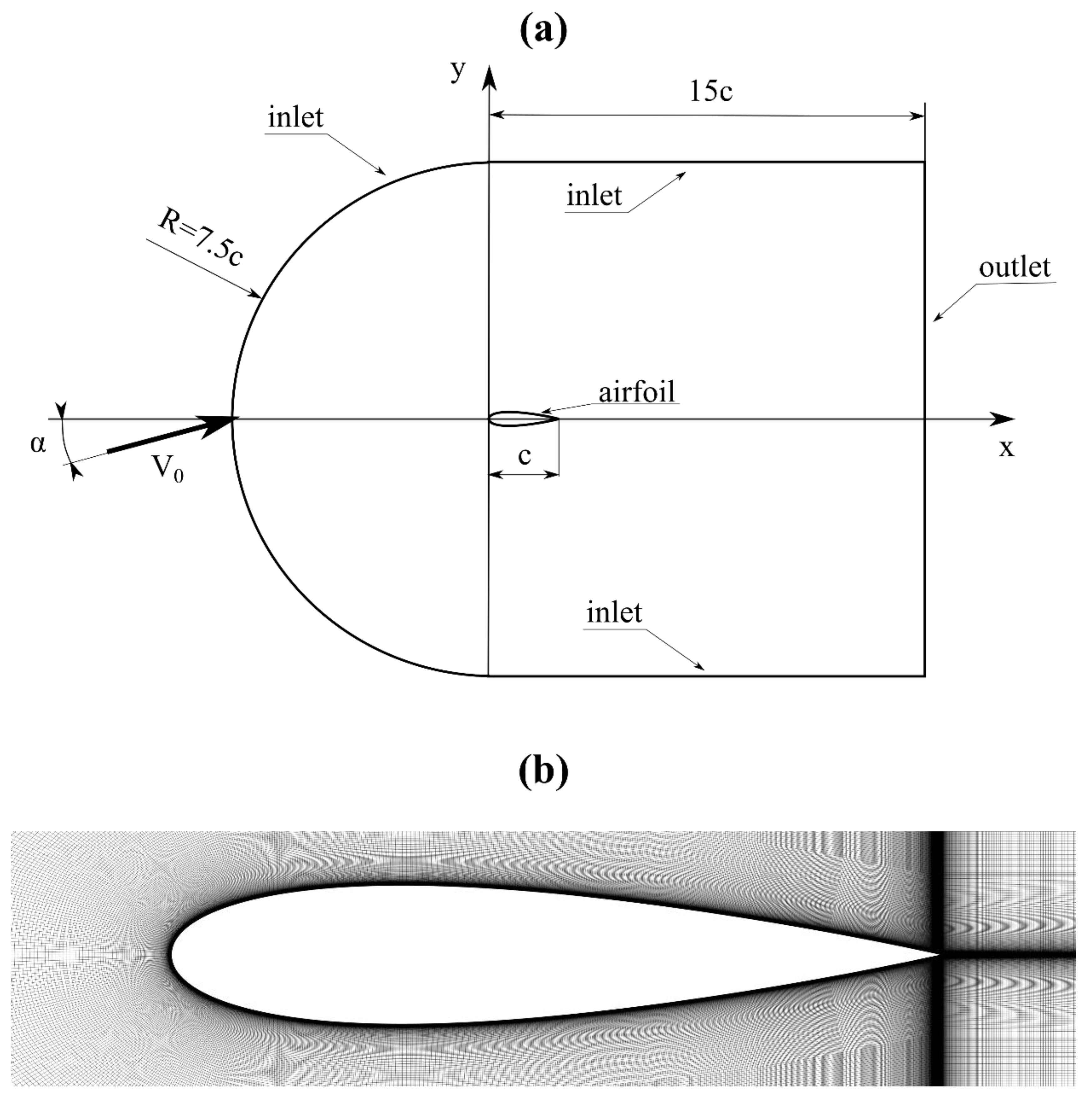
2.1. Numerical Domain and CFD Solver Settings
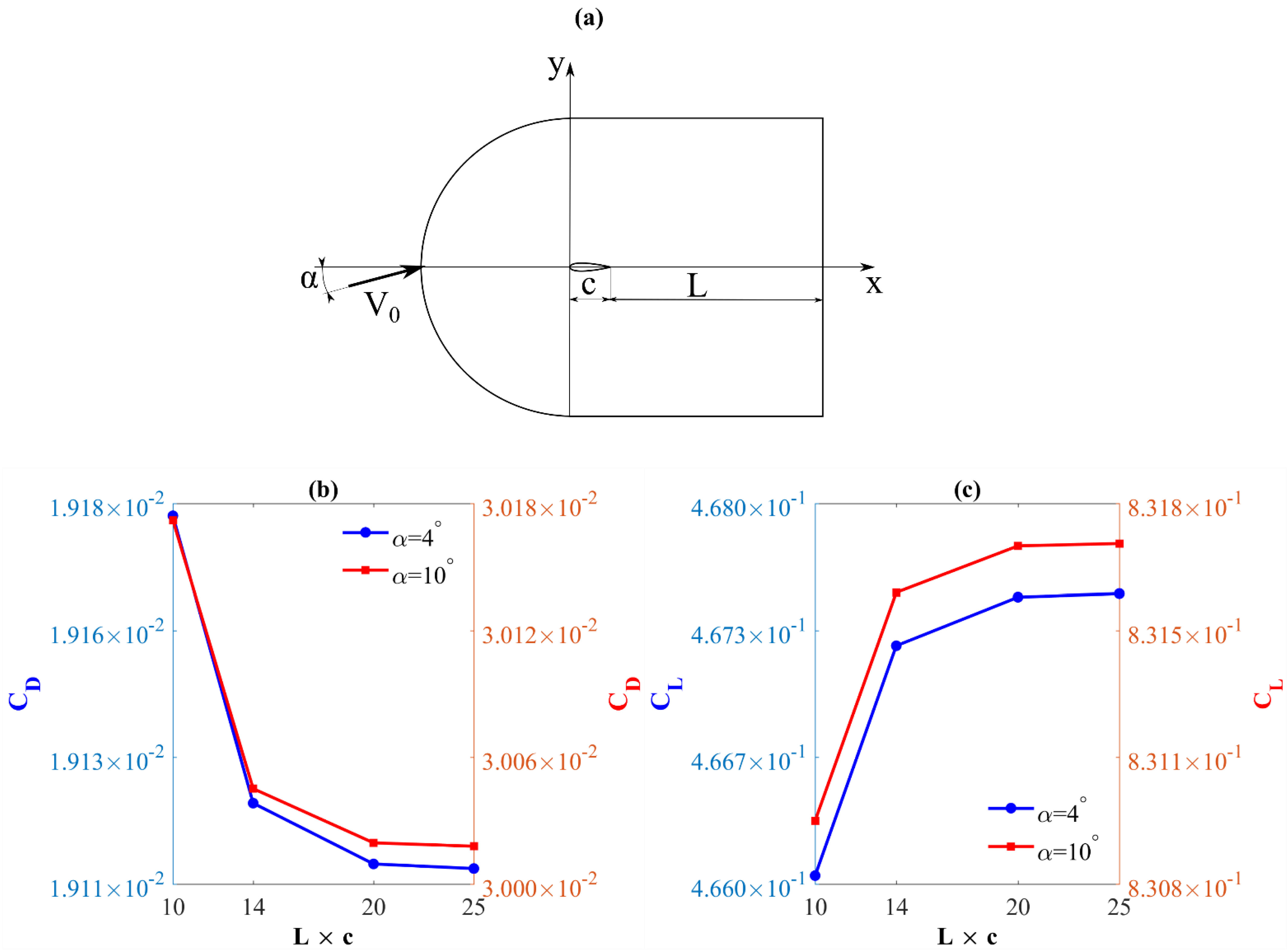
2.2. Computing Domain Size Effect
2.3. Turbulence Intensity Effect and Mesh Sensitivity Studies
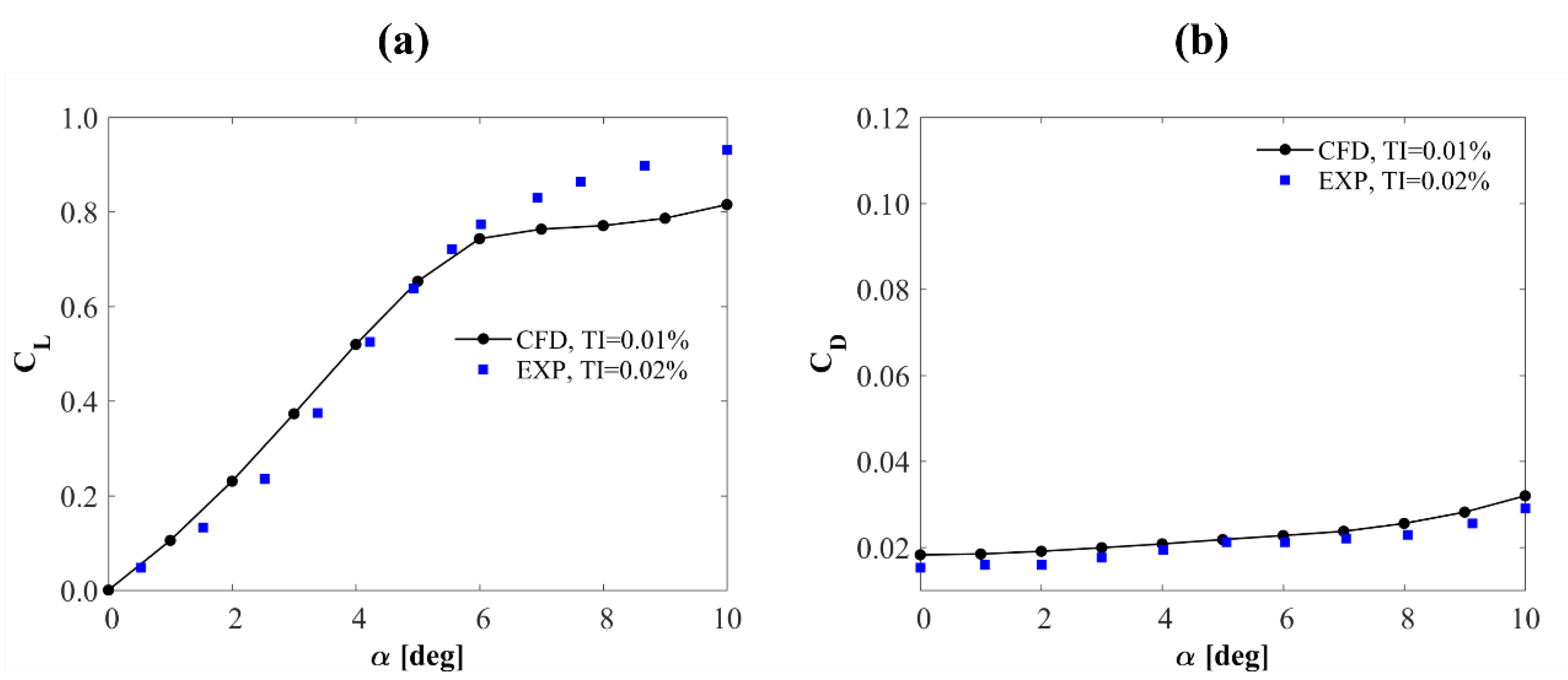
2.4. Validation of the Numerical Model
3. Results
3.1. Reynolds Number Effect on Lift and Drag Coefficients
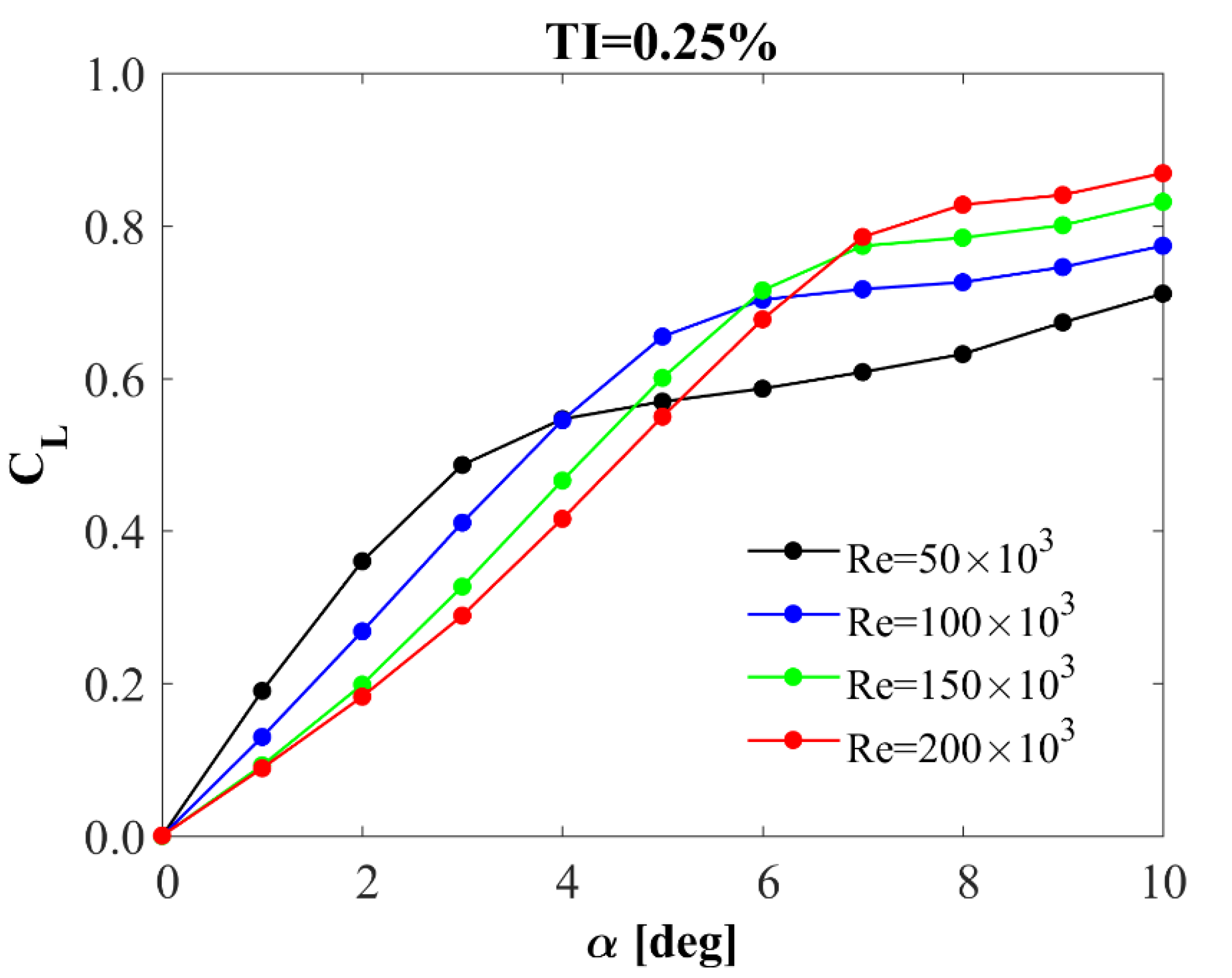
3.1.1. Lift Force Coefficient
3.1.2. Drag Force Coefficient
3.2. Turbulence Intensity Effect on Lift and Drag Coefficients
3.2.1. Lift Force Coefficient
- 1.
- An increase in TI causes a decrease in the derivative in the first area, an increase in the derivative in the second area, and an increase in .
- 2.
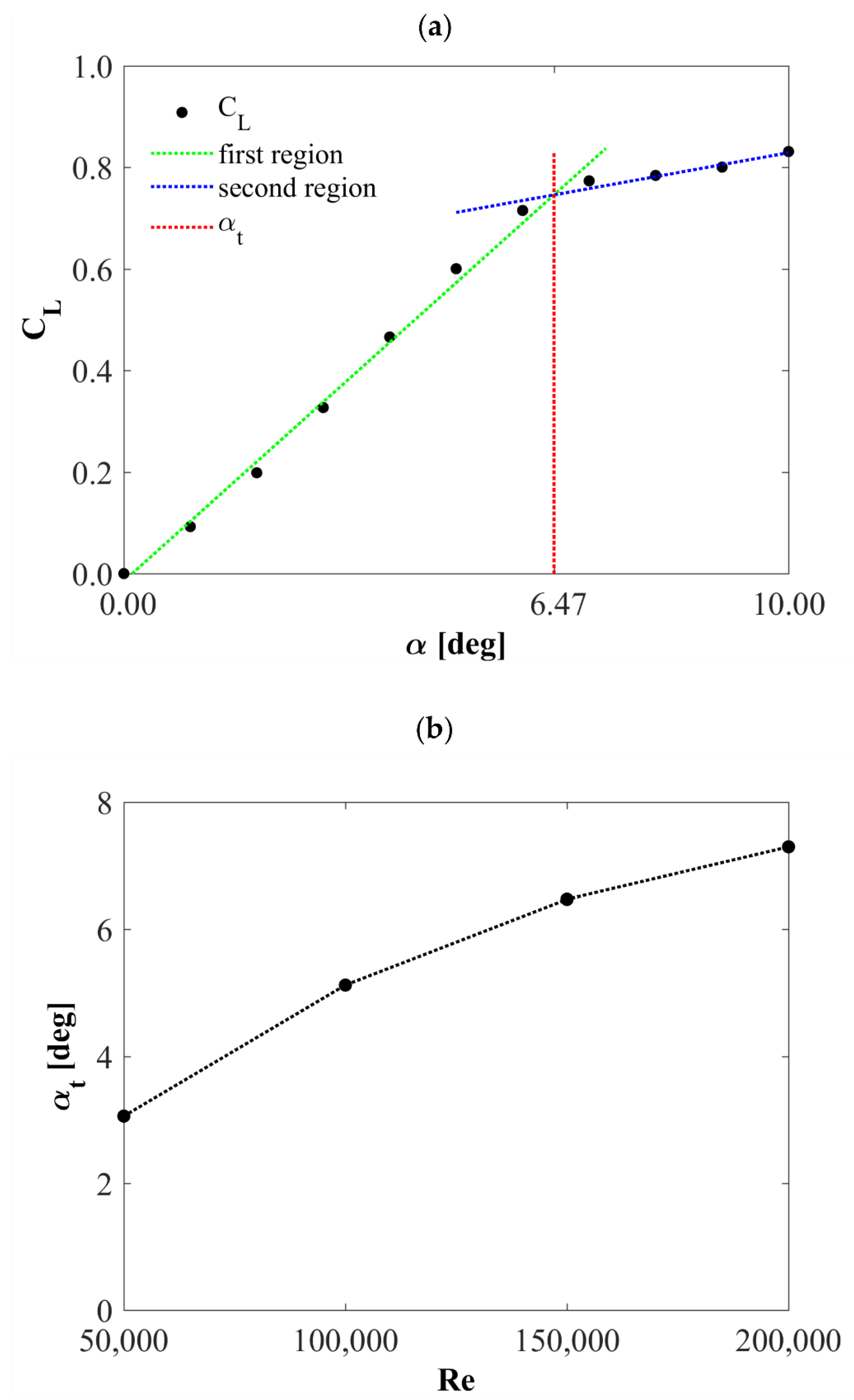
- An increase in Re causes a decrease in the derivative in the first region and an almost linear increase in the angle.
- 3.
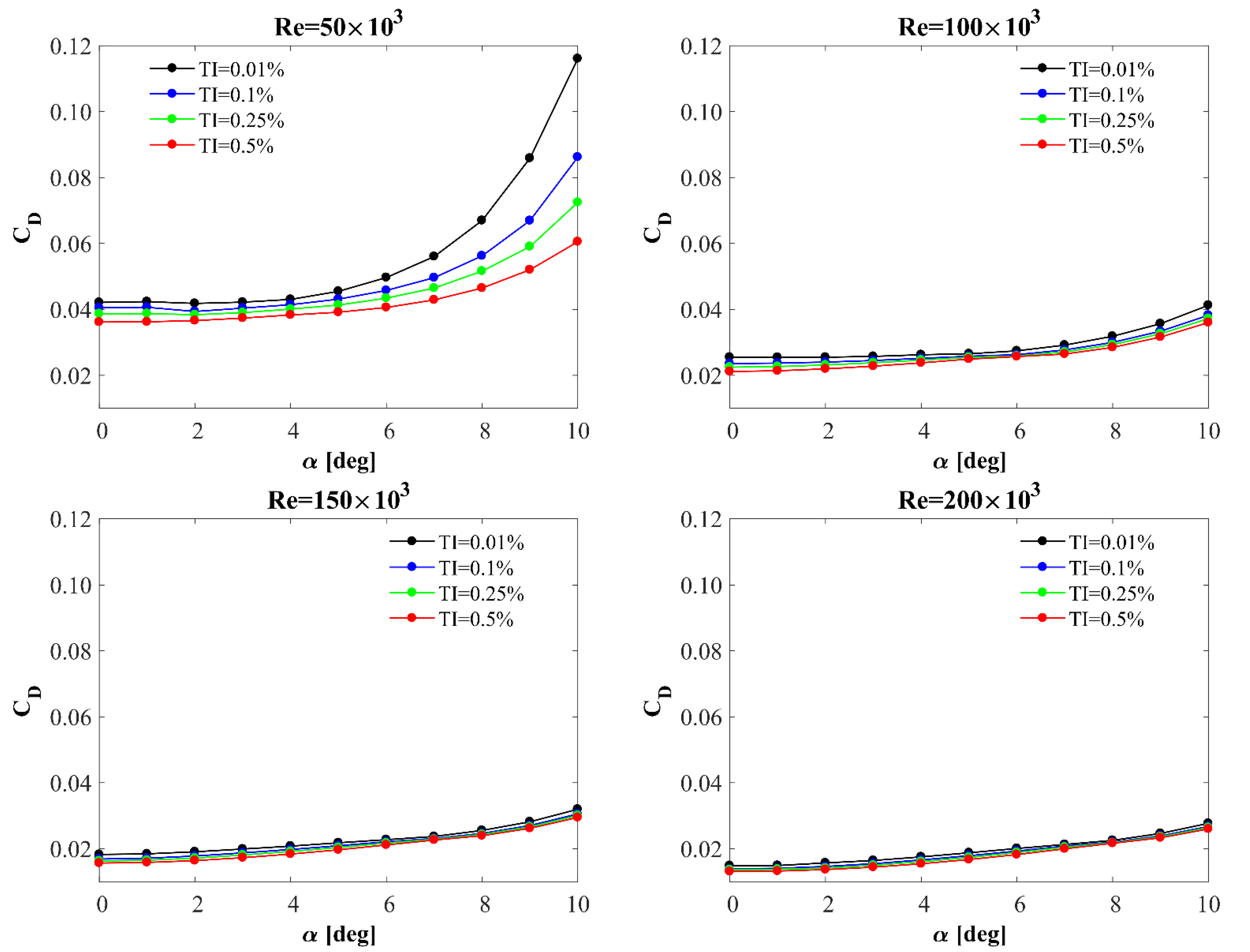
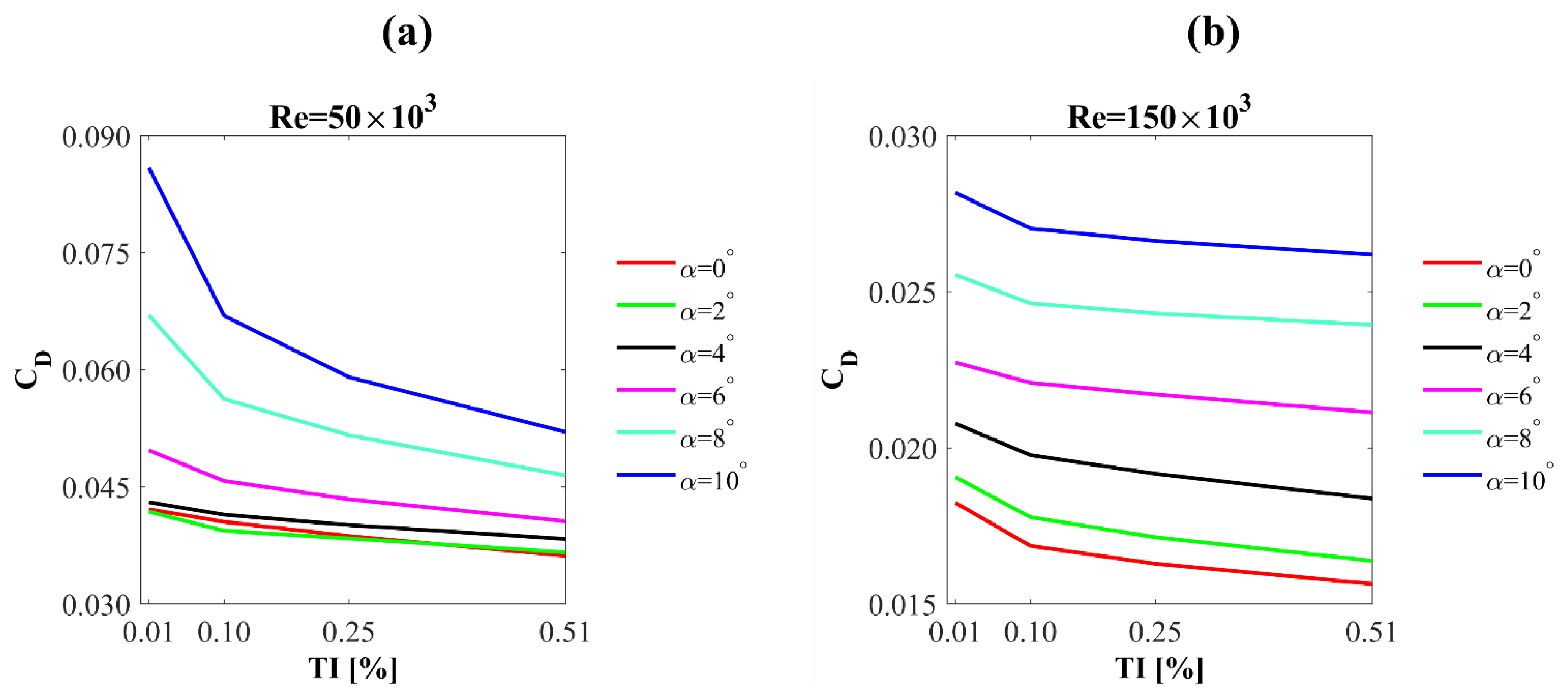
3.2.2. Drag Force
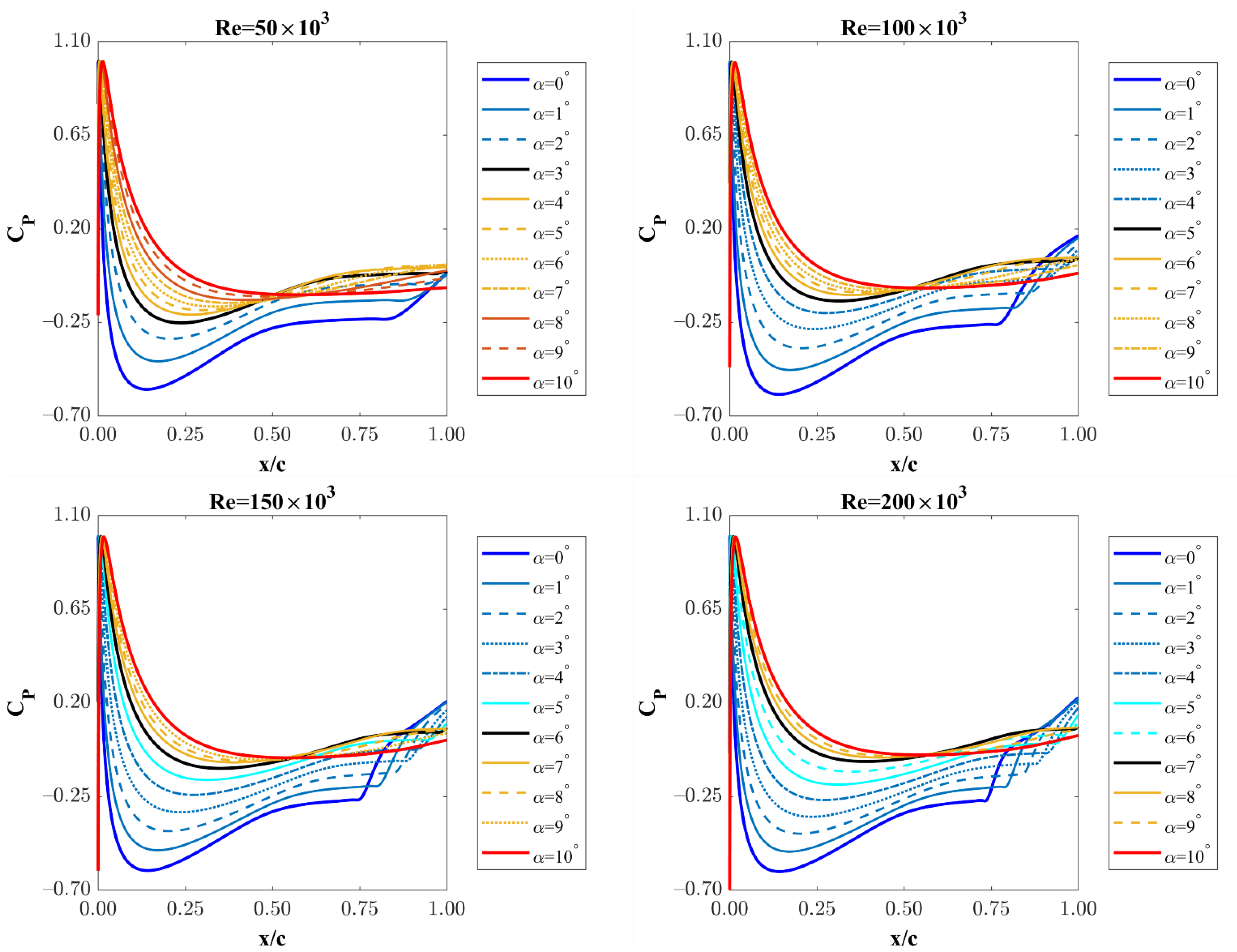
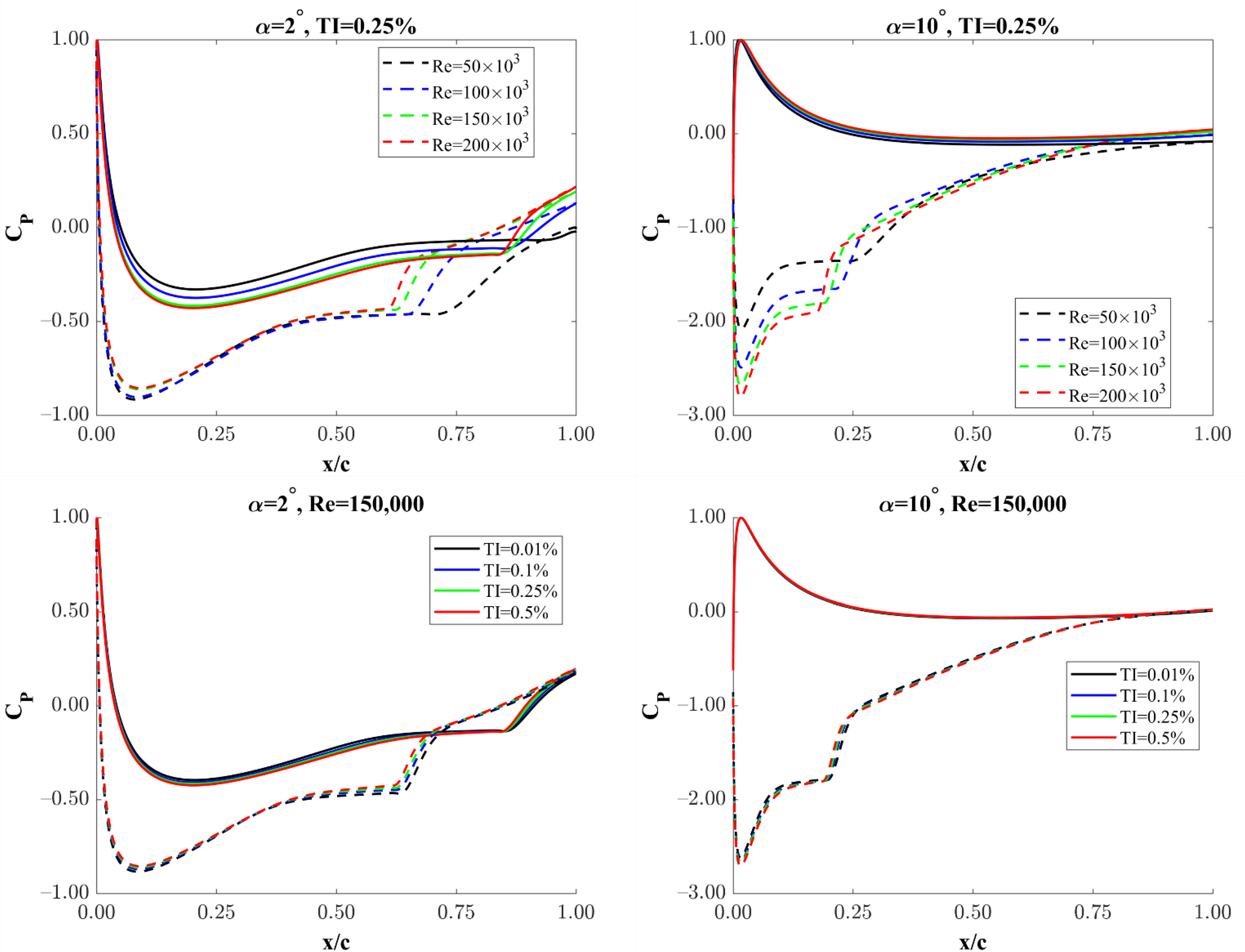
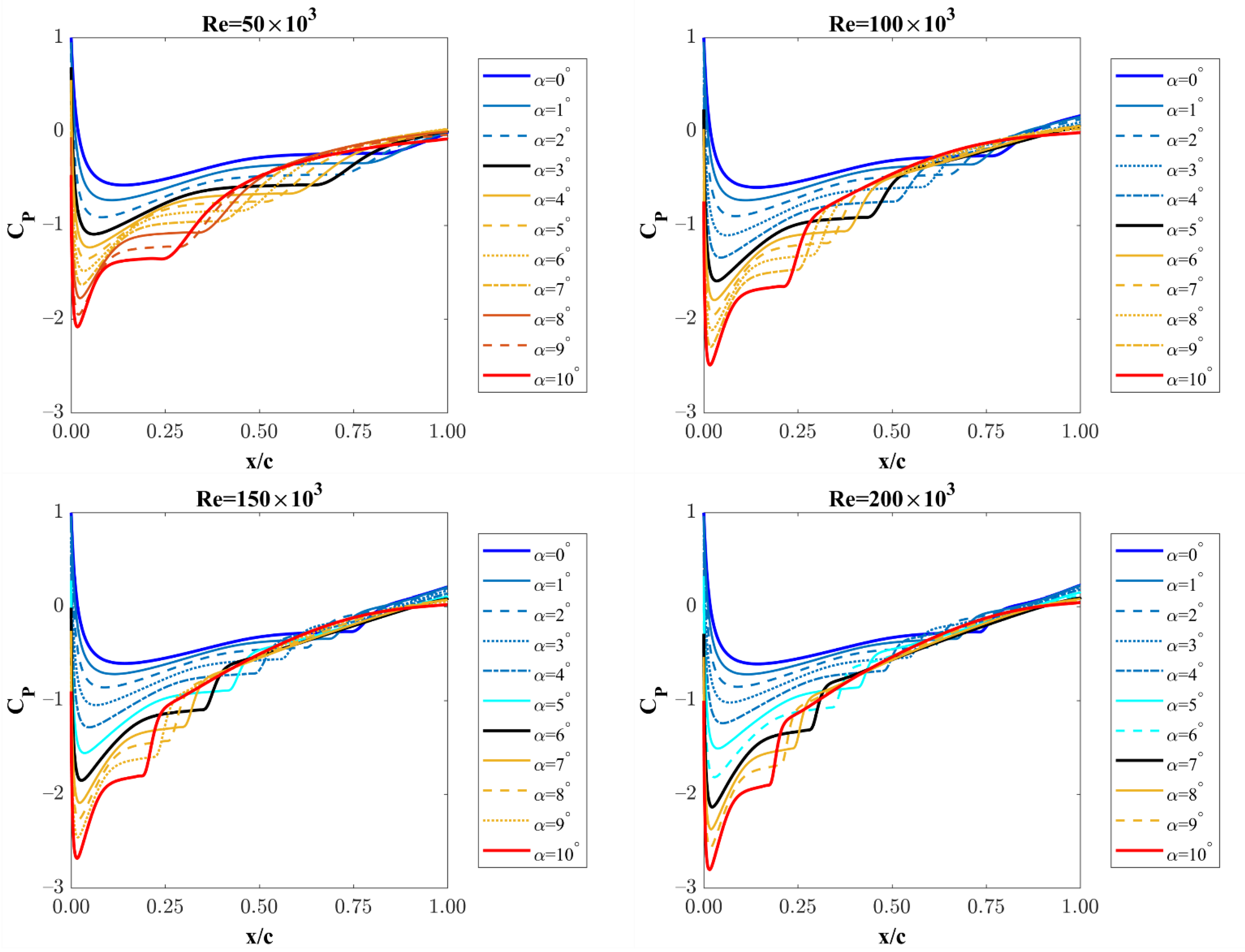
3.3. Static Pressure
4. Conclusions
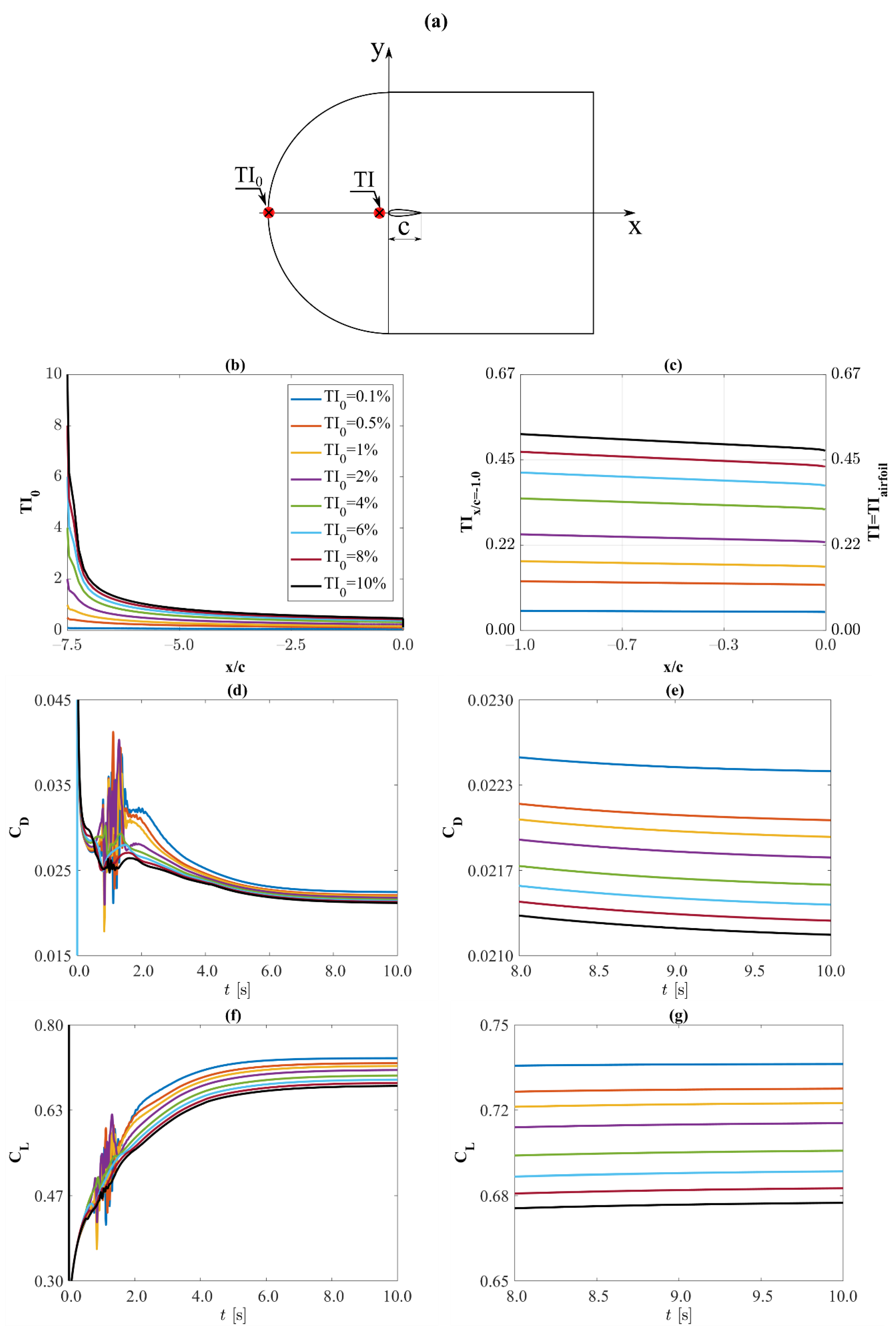
- One of the key achievements of this paper is the analysis of the aerodynamic characteristics of the NACA 0018 airfoil in relation to the turbulence intensity. The decay rate of turbulence intensity strongly depends on the turbulence intensity at the inlet. The higher the turbulence intensity at the inlet, the higher the decay rate. For the lowest turbulence intensity analyzed in this work, equal to 0.1%, the decay rate is almost constant. In the vicinity of the nose of the profile, the turbulence intensity is very low regardless of the inlet’s turbulence intensity. The results shown in Figure 4b,c have practical applications when using the mesh described in the paper [6]. The data shown in these graphs can be used to interpolate the turbulence intensity at the inlet in order to obtain a specific value of the turbulence intensity on the airfoil.
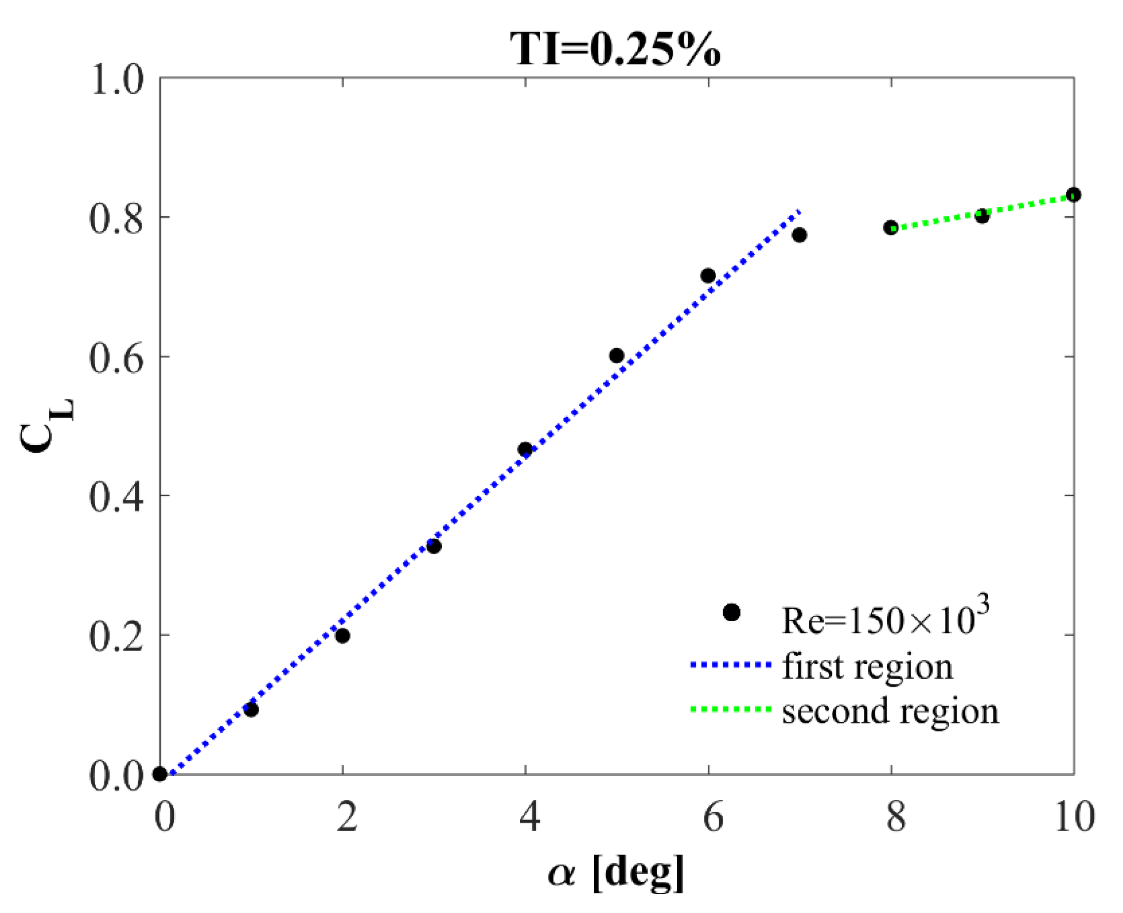
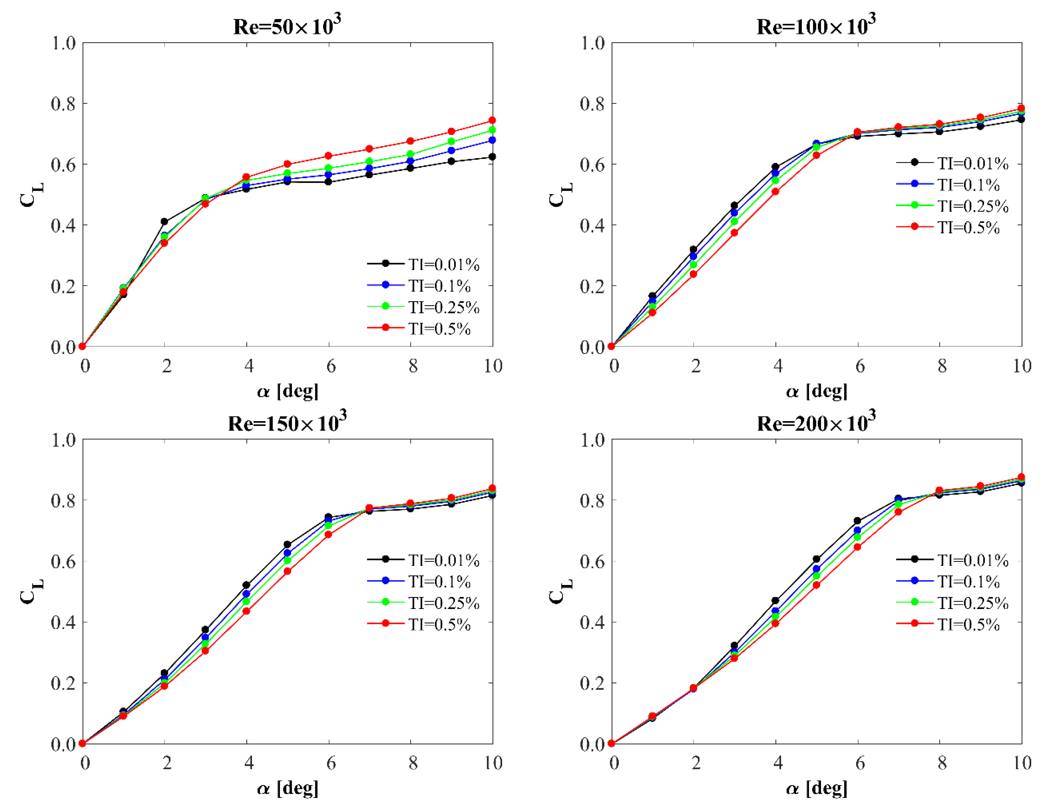
- All calculations carried out in this paper, regardless of the Reynolds number and the turbulent intensity, showed a zero-lift coefficient at a zero angle of attack.
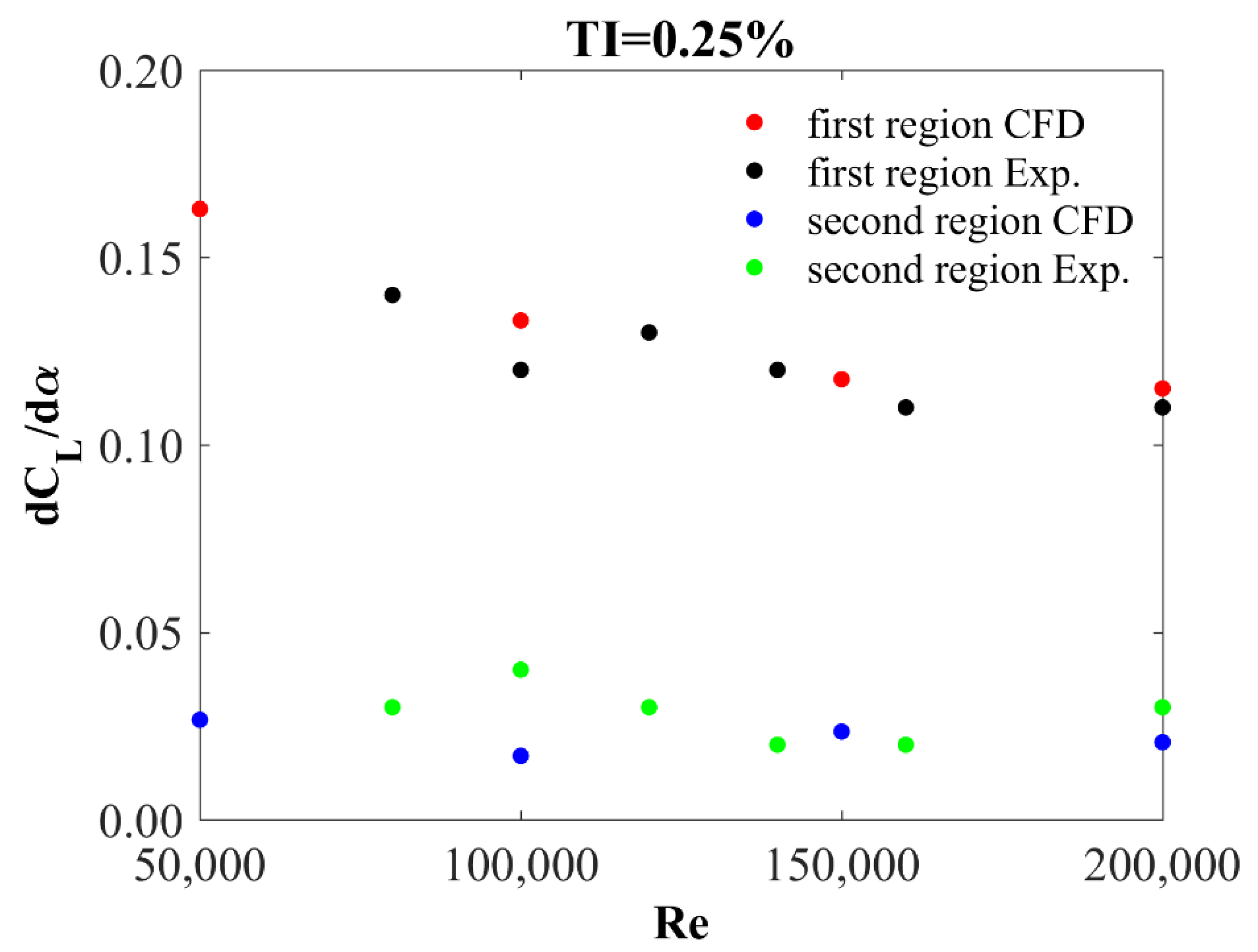
- The presence of a wide laminar-separation bubble in the boundary layer results in the occurrence of two aerodynamic derivatives of the lift coefficient in the range of angles of attack before stall. The increase in Reynolds number primarily causes a linear increase in the first region. On the other hand, the aerodynamic derivative in the second region is almost independent of the Reynolds number.
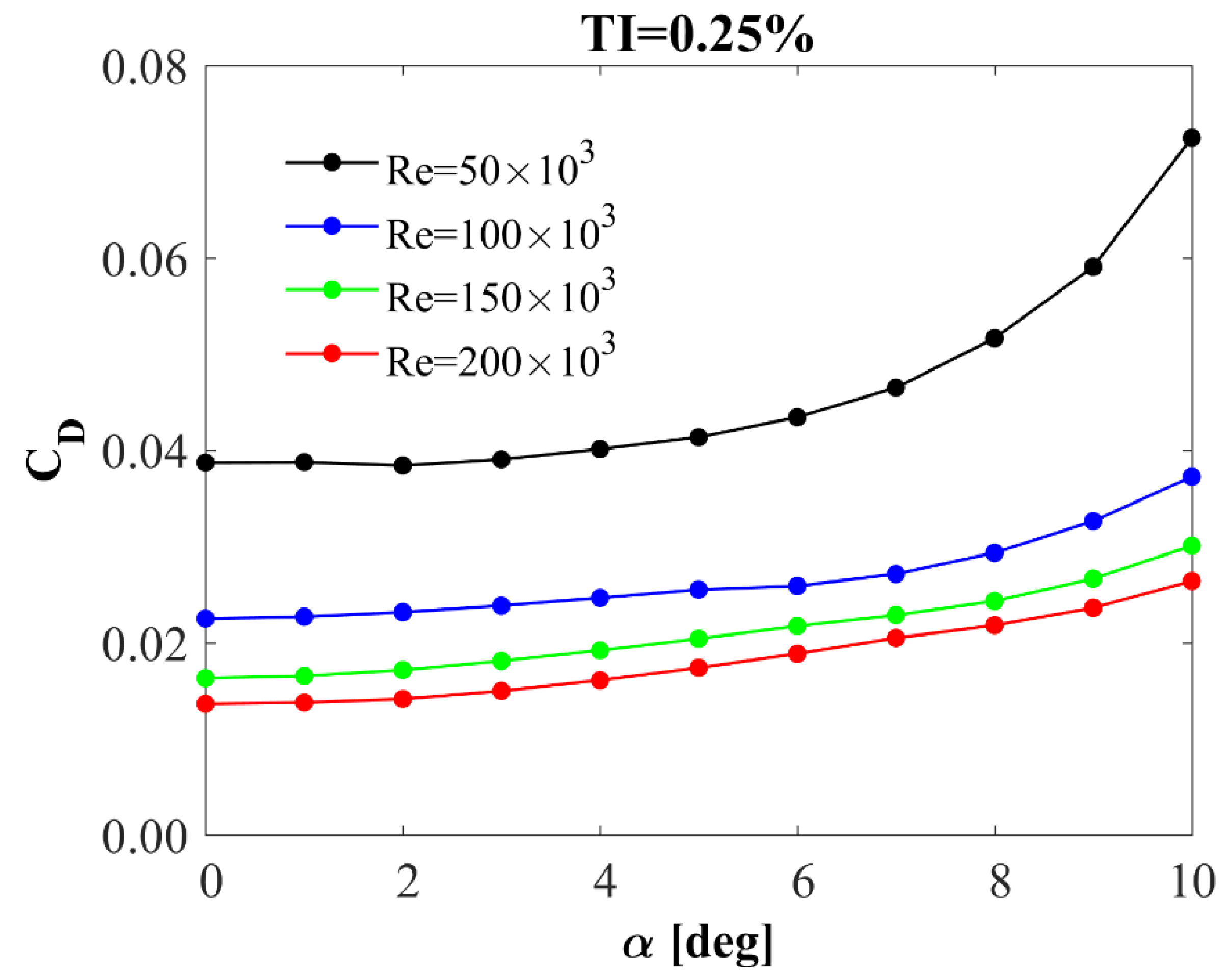
- At a Reynolds number of 50,000, a faster increase in drag is observed starting from an angle of attack of 6 deg. For higher Reynolds numbers, the increase in drag coefficient as a function of the angle of attack is much smoother. The drag coefficients differ very little for low angles of attack and Reynolds numbers higher than 100,000.
- Generally, the effect of the turbulence intensity on the lift coefficient is much lower than the Reynolds number effect. The increase in turbulence intensity causes the lift coefficient to decrease in the first region and increase in the second region. Differences in lift coefficients for high angles of attack decrease with increasing the Reynolds number and the turbulence intensity.
- The increase in turbulence intensity causes a decrease in the aerodynamic derivative in the first region and its increase in the second region. Increasing turbulence intensity also increases the transition angle of attack. This trend is visible for all the Reynolds numbers studied in this work.
- For angles of attack higher than the transition angle of attack, there is no longer a laminar-separation bubble on the pressure surface of the airfoil.
- Drag coefficients are less sensitive to the turbulence intensity than the lift coefficients, except for the lowest investigated Reynolds number of 50,000. In general, an increase in the angle of attack causes an increase in the drag coefficient.
- The Reynolds number has a much greater effect on the pressure distributions than the turbulence intensity. The effect of Reynolds number and turbulence intensity is much greater on the suction side of the profile.
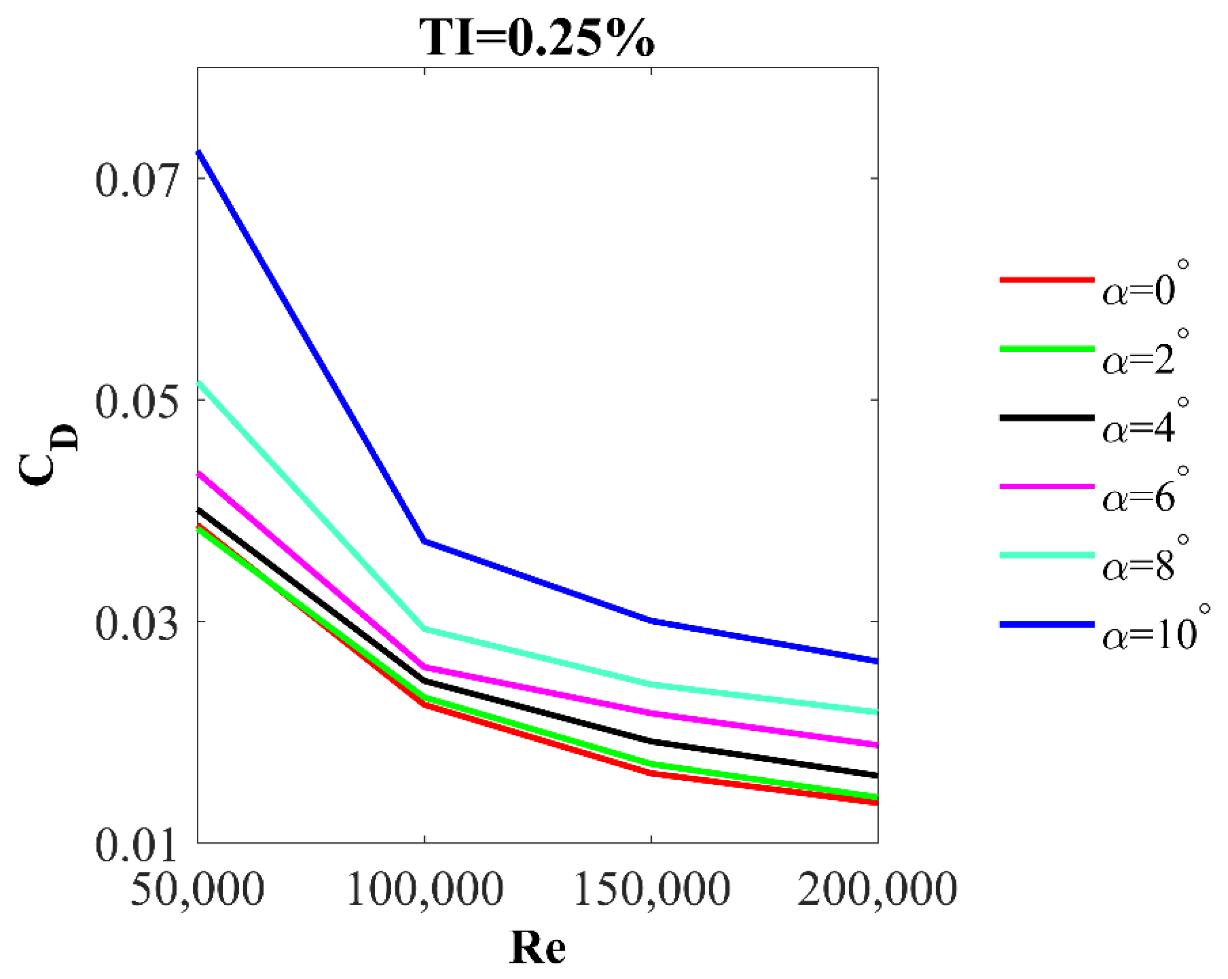
- The performed numerical analyzes showed clear differences in the characteristics of the drag coefficient for a Reynolds number of 50,000. For the other considered Reynolds numbers in the range of 100,000 to 200,000, the changes in the drag coefficients are rather linear as a function of both the turbulence intensity and the Reynolds number.
Author Contributions
Funding
Institutional Review Board Statement
Informed Consent Statement
Data Availability Statement
Conflicts of Interest
Nomenclature
| chord length | |
| drag coefficient | |
| lift coefficient | |
| static pressure coefficient | |
| rate of change of lift coefficient with angle of attack | |
| turbulence length scale | |
| length from the airfoil’s trailing edge to the domain’s outlet boundary | |
| chord-based Reynolds number | |
| turbulence intensity on the airfoil | |
| inlet turbulence intensity | |
| free stream wind velocity [m/s] | |
| angle of attack | |
| transition angle of attack (the angle between the first and the second region) | |
| boundary-layer thickness |
References
- Lin, J.M.; Pauley, L.L. Low-Reynolds-number separation on an airfoil. AIAA J. 1996, 34, 1570–1577. [Google Scholar] [CrossRef]
- Bangga, G.; Dessoky, A.; Wu, Z.; Rogowski, K.; Hansen, M.O.L. Accuracy and consistency of CFD and engineering models for simulating vertical axis wind turbine loads. Energy 2020, 206, 118087. [Google Scholar] [CrossRef]
- Ramírez, J.M.; Saravia, M. Assessment of Reynolds-averaged Navier–Stokes method for modeling the startup regime of a Darrieus rotor. Phys. Fluids 2021, 33, 037125. [Google Scholar] [CrossRef]
- Branlard, E.; Brownstein, I.; Strom, B.; Jonkman, J.; Dana, S.; Baring-Gould, E.I. A multipurpose lifting-line flow solver for arbitrary wind energy concepts. Wind Energ. Sci. 2022, 7, 455–467. [Google Scholar] [CrossRef]
- Silva, J.E.; Danao, L.A.M. Varying VAWT Cluster Configuration and the Effect on Individual Rotor and Overall Cluster Performance. Energies 2021, 14, 1567. [Google Scholar] [CrossRef]
- Rogowski, K.; Królak, G.; Bangga, G. Numerical Study on the Aerodynamic Characteristics of the NACA 0018 Airfoil at Low Reynolds Number for Darrieus Wind Turbines Using the Transition SST Model. Processes 2021, 9, 477. [Google Scholar] [CrossRef]
- Paraschivoiu, I. Wind Turbine Design: With Emphasis on Darrieus Concept; Polytechnic International Press: Montreal, QC, Canada, 2002. [Google Scholar]
- Martinez, J.; Bernabini, L.; Probst, O.; Rodriguez, C. An improved BEM model for the power curve prediction of stall-regulated wind turbines. Wind Energy 2005, 8, 385–402. [Google Scholar] [CrossRef]
- Hansen, M.O.L. Aerodynamics of Wind Turbines; Earthscan Publications Ltd.: London, UK, 2008. [Google Scholar]
- Zhang, Z.; Nielsen, S.R.K.; Blaabjerg, F.; Zhou, D. Dynamics and Control of Lateral Tower Vibrations in Offshore Wind Turbines by Means of Active Generator Torque. Energies 2014, 7, 7746–7772. [Google Scholar] [CrossRef]
- Fernandez-Gamiz, U.; Zulueta, E.; Boyano, A.; Ansoategui, I.; Uriarte, I. Five Megawatt Wind Turbine Power Output Improvements by Passive Flow Control Devices. Energies 2017, 10, 742. [Google Scholar] [CrossRef] [Green Version]
- Żugaj, M.; Bibik, P.; Jacewicz, M. UAV aircraft model for control system failures analysis. J. Theor. Appl. Mech. 2016, 54, 1405–1415. [Google Scholar] [CrossRef] [Green Version]
- Jimenez, P.; Lichota, P.; Agudelo, D.; Rogowski, K. Experimental Validation of Total Energy Control System for UAVs. Energies 2020, 13, 14. [Google Scholar] [CrossRef] [Green Version]
- Sheng, H.; Zhang, C.; Xiang, Y. Mathematical Modeling and Stability Analysis of Tiltrotor Aircraft. Drones 2022, 6, 92. [Google Scholar] [CrossRef]
- El-Fahham, I.; Abdelshahid, G.; Mokhiamar, O. Pitch Angle Modulation of the Horizontal and Vertical Axes Wind Turbine Using Fuzzy Logic Control. Processes 2021, 9, 1337. [Google Scholar] [CrossRef]
- Sakamoto, L.; Fukui, T.; Morinishi, K. Blade Dimension Optimization and Performance Analysis of the 2-D Ugrinsky Wind Turbine. Energies 2022, 15, 2478. [Google Scholar] [CrossRef]
- Ghiasi, P.; Najafi, G.; Ghobadian, B.; Jafari, A.; Mazlan, M. Analytical Study of the Impact of Solidity, Chord Length, Number of Blades, Aspect Ratio and Airfoil Type on H-Rotor Darrieus Wind Turbine Performance at Low Reynolds Number. Sustainability 2022, 14, 2623. [Google Scholar] [CrossRef]
- Ferreira, C.S.; Madsen, H.A.; Barone, M.; Roscher, B.; Deglaire, P.; Arduin, I. Comparison of aerodynamic models for Vertical Axis Wind Turbines. J. Phys. Conf. Ser. 2014, 524, 012125. [Google Scholar] [CrossRef]
- Castelein, D.; Ragni, D.; Tescione, G.; Ferreira, C.J.S.; Gaunaa, M. Creating a benchmark of Vertical Axis Wind Turbines in Dynamic Stall for validating numerical models. In Proceedings of the 33rd Wind Energy Symposium, AIAA SciTech, AIAA 2015-0723, Kissimmee, FL, USA, 5–9 January 2015. [Google Scholar] [CrossRef]
- Rogowski, K.; Hansen, M.O.L.; Bangga, G. Performance Analysis of a H-Darrieus Wind Turbine for a Series of 4-Digit NACA Airfoils. Energies 2020, 13, 3196. [Google Scholar] [CrossRef]
- Lichota, P. Multi-Axis Inputs for Identification of a Reconfigurable Fixed-Wing UAV. Aerospace 2020, 7, 113. [Google Scholar] [CrossRef]
- Lichota, P.; Norena, D.A. A Priori Model Inclusion in the Multisine Maneuver Design. In Proceedings of the 17th International Carpathian Control Conference, High Tatras, Slovakia, 29 May–1 June 2016; Petras, I., Podlubny, I., Kacur, J., Eds.; IEEE: Tatranská Lomnica, Slovakia, 2016; pp. 440–445. [Google Scholar] [CrossRef]
- ANSYS, Inc. ANSYS Fluent Theory Guide, Release 19.1.; ANSYS, Inc.: Canonsburg, PA, USA, 2019. [Google Scholar]
- Timmer, W.A. Two-Dimensional Low-Reynolds Number Wind Tunnel Results for Airfoil NACA 0018. Wind. Eng. 2008, 32, 525–537. [Google Scholar] [CrossRef] [Green Version]
- Dul, F.; Lichota, P.; Rusowicz, A. Generalized Linear Quadratic Control for a Full Tracking Problem in Aviation. Sensors 2020, 20, 2955. [Google Scholar] [CrossRef]
- Ren, G.; Liu, J.; Wan, J.; Li, F.; Guo, Y.; Yu, D. The analysis of turbulence intensity based on wind speed data in onshore wind farms. Renew. Energy 2018, 123, 756–766. [Google Scholar] [CrossRef]
- Laneville, A.; Vittecoq, P. Dynamic stall: The case of the vertical axis wind turbine. J. Sol. Energy Eng. 1986, 108, 140–145. [Google Scholar] [CrossRef]
- Rogowski, K.; Maroński, R.; Hansen, M.O.L. Steady and unsteady analysis of NACA 0018 airfoil in vertical-axis wind turbine. J. Theor. Appl. Mech. 2018, 51, 203–212. [Google Scholar] [CrossRef] [Green Version]
- Yang, Y.; Guo, Z.; Zhang, Y.; Jinyama, H.; Li, Q. Numerical Investigation of the Tip Vortex of a Straight-Bladed Vertical Axis Wind Turbine with Double-Blades. Energies 2017, 10, 1721. [Google Scholar] [CrossRef] [Green Version]
- Mohan Kumar, P.; Sivalingam, K.; Lim, T.-C.; Ramakrishna, S.; Wei, H. Strategies for Enhancing the Low Wind Speed Performance of H-Darrieus Wind Turbine—Part 1. Clean Technol. 2019, 1, 185–204. [Google Scholar] [CrossRef] [Green Version]
- Rogowski, K. CFD Computation of the H-Darrieus Wind Turbine—The Impact of the Rotating Shaft on the Rotor Performance. Energies 2019, 12, 2506. [Google Scholar] [CrossRef] [Green Version]
- Rogowski, K.; Hansen, M.O.L.; Maroński, R.; Lichota, P. Scale Adaptive Simulation Model for the Darrieus Wind Turbine. J. Phys. Conf. Ser. 2016, 753, 022050. [Google Scholar] [CrossRef]
- Alaimo, A.; Esposito, A.; Messineo, A.; Orlando, C.; Tumino, D. 3D CFD Analysis of a Vertical Axis Wind Turbine. Energies 2015, 8, 3013–3033. [Google Scholar] [CrossRef] [Green Version]
- Jacobs, N.E.; Ward, K.E.; Pinkerton, R.M. The Characteristics of 78 Related Airfoil Sections from Tests in the Variable-Density Wind Tunnel. In NACA Report 460; Langley Memorial Aeronautical Laboratory: Hampton, VA, USA, 1933; ISBN NACA-460. Available online: https://ntrs.nasa.gov/api/citations/19930091108/downloads/19930091108.pdf (accessed on 15 April 2022).
- Anderson, J.D., Jr. Fundamentals of Aerodynamics, 5th ed.; McGraw-Hill: New York, NY, USA, 2011. [Google Scholar]
- Moran, J. An Introduction to Theoretical and Computational Aerodynamics, 1st ed.; John Wiley & Sons: New York, NY, USA, 1984. [Google Scholar]
- Królak, G. Numerical Analysis of Aerodynamic Characteristics of the NACA 0018 Airfoil Used in the Darrieus wind Turbines. Master’s Thesis, The Faculty of Power and Aeronautical Engineering, Warsaw University of Technology, Warsaw, Poland, 2020. [Google Scholar]
- Ferreira, C.S.; Barone, M.; Zanon, A.; Giannattasio, P. Airfoil optimization for stall regulated vertical axis wind turbines. In Proceedings of the AIAA SciTech—33rd Wind Energy Symposium, Kissimmee, FL, USA, 5–9 January 2015; pp. 1–16. [Google Scholar] [CrossRef]
- Ashwill, T.D. Measured Data for the Sandia 34-Meter Vertical Axis Wind Turbine; SAND91-2228; Sandia National Laboratories: Albuquerque, NM, USA, 1992. [Google Scholar]
- Shires, A. Development and Evaluation of an Aerodynamic Model for a Novel Vertical Axis Wind Turbine Concept. Energies 2013, 6, 2501–2520. [Google Scholar] [CrossRef] [Green Version]
- Jacobs, E.N.; Sherman, A. Airfoil Section Characteristics as Affected by Variations of the Reynolds Number; Technical Report; National Advisory Committee for Aeronautics: Langley Field, VA, USA, 1937. Available online: https://ntrs.nasa.gov/api/citations/19930091662/downloads/19930091662.pdf (accessed on 15 April 2022).
- Abbott, H.; Doenhoff, E.; Lous, S.; Stivers, J. National Advisory Commitee for Aeronautics Report No. 824: Summary of Airfoil Data. 1945. Available online: https://ntrs.nasa.gov/api/citations/19930090976/downloads/19930090976.pdf (accessed on 15 April 2022).
- Sheldahl, R.E.; Klimas, P.C. Aerodynamic Characteristics of Seven Symmetrical Airfoil Sections through 180-Degree Angle of Attack for Use in Aerodynamic Analysis of Vertical Axis Wind Turbines; Technical Report; Sandia National Laboratories: Albuquerque, NM, USA, 1981. [Google Scholar] [CrossRef] [Green Version]
- Bastankhah, M.; Porté-Agel, F. A New Miniature Wind Turbine for Wind Tunnel Experiments. Part I: Design and Performance. Energies 2017, 10, 908. [Google Scholar] [CrossRef] [Green Version]
- Hezaveh, S.H.; Bou-Zeid, E.; Lohry, M.W.; Martinelli, L. Simulation and wake analysis of a single vertical axis wind turbine. Wind Energy 2017, 20, 713–730. [Google Scholar] [CrossRef]
- Bedon, G.; Schmidt Paulsen, U.; Aagaard Madsen, H.; Belloni, F.; Raciti Castelli, M.; Benini, E. Computational assessment of the DeepWind aerodynamic performance with different blade and airfoil configurations. Appl. Energy 2017, 185, 1100–1108. [Google Scholar] [CrossRef]
- Rossander, M.; Dyachuk, E.; Apelfröjd, S.; Trolin, K.; Goude, A.; Bernhoff, H.; Eriksson, S. Evaluation of a Blade Force Measurement System for a Vertical Axis Wind Turbine Using Load Cells. Energies 2015, 8, 5973–5996. [Google Scholar] [CrossRef] [Green Version]
- Shires, A.; Kourkoulis, V. Application of Circulation Controlled Blades for Vertical Axis Wind Turbines. Energies 2013, 6, 3744–3763. [Google Scholar] [CrossRef]
- Nakano, T.; Fujisawa, N.; Oguma, Y.; Takagi, Y.; Lee, S. Experimental study on flow and noise characteristics of NACA0018 airfoil. J. Wind. Eng. Ind. Aerodyn. 2007, 95, 511–531. [Google Scholar] [CrossRef]
- Bianchini, A.; Balduzzi, F.; Rainbird, J.M.; Peiro, J.; Graham, J.M.R.; Ferrara, G.; Ferrari, L. An Experimental and Numerical Assessment of Airfoil Polars for Use in Darrieus Wind Turbines—Part I: Flow Curvature Effects. J. Eng. Gas Turbine Power 2016, 138, 032602. [Google Scholar] [CrossRef]
- Bianchini, A.; Balduzzi, F.; Rainbird, J.M.; Peiro, J.; Graham, J.M.R.; Ferrara, G.; Ferrari, L. An Experimental and Numerical Assessment of Airfoil Polars for Use in Darrieus Wind Turbines—Part II: Post-stall Data Extrapolation Methods. J. Eng. Gas. Turbine Power 2016, 138, 032603. [Google Scholar] [CrossRef]
- Istvan, M. Turbulence intensity effects on laminar separation bubbles formed over an airfoil. AIAA J. 2018, 56, 335–1347. [Google Scholar] [CrossRef]
- Istvan, M.S.; Yarusevych, S. Effects of free-stream turbulence intensity on transition in a laminar separation bubble formed over an airfoil. Exp. Fluids 2018, 59, 52. [Google Scholar] [CrossRef]
- Claessens, M.C. The Design and Testing of Airfoils in Small Vertical Axis Wind Turbines. Master’s Thesis, Delft University of Technology, Delft, The Netherlands, 2006. Available online: https://repository.tudelft.nl/islandora/object/uuid%3Afe4a7ae3-103e-40f3-a1f1-ae6d910d8c71 (accessed on 10 April 2022).
- Du, L. Numerical and Experimental Investigations of Darrieus Wind Turbine Start-up and Operation. Ph.D. Thesis, Durham University, Durham, UK, 2016. Available online: http://etheses.dur.ac.uk/11384/ (accessed on 10 April 2022).
- Müller-Vahl, H.F.; Strangfeld, C.; Nayeri, C.; Paschereit, C.O.; Greenblatt, D. Control of Thick Airfoil, Deep Dynamic Stall Using Steady Blowing. AIAA J. 2015, 53, 277–295. [Google Scholar] [CrossRef]
- Melani, P.F.; Balduzzi, F.; Ferrara, G.; Bianchini, A. An Annotated Database of Low Reynolds Aerodynamic Coefficients for the NACA0018 Airfoil. AIP Conf. Proc. 2019, 2191, 020110. [Google Scholar] [CrossRef]
- Belabes, B.; Paraschivoiu, M. Numerical study of the effect of turbulence intensity on VAWT performance. Energy 2021, 233, 121139. [Google Scholar] [CrossRef]
- Tangermann, E.; Klein, M. Numerical simulation of laminar separation on a NACA0018 airfoil in freestream turbulence. In Proceedings of the AIAA Scitech 2020 Forum, Orlando, FL, USA, 6–10 January 2020; pp. 1–10. [Google Scholar] [CrossRef]
- Marxen, O.; Rist, U.; Wagner, S. Effect of spanwise-modulated disturbances on transition in a separated boundary layer. AIAA J. 2004, 42, 937–944. [Google Scholar] [CrossRef]
- Galbraith, M.C.; Visbal, M.R. Implicit Large Eddy Simulation of Low-Reynolds-Number Transitional Flow Past the SD7003 Airfoil. In Proceedings of the 40th Fluid Dynamics Conference and Exhibit, Chicago, IL, USA, 28 June–1 July 2010. [Google Scholar] [CrossRef] [Green Version]
- Zhiyin, Y. Large-eddy simulation: Past, present and the future. Chin. J. Aeronaut. 2015, 28, 11–24. [Google Scholar] [CrossRef] [Green Version]
- Kim, J.-H.; Ahn, J. Large Eddy Simulation of Leakage Flow in a Stepped Labyrinth Seal. Processes 2021, 9, 2179. [Google Scholar] [CrossRef]
- Huang, Z.; Shi, G.; Liu, X.; Wen, H. Effect of Flow Rate on Turbulence Dissipation Rate Distribution in a Multiphase Pump. Processes 2021, 9, 886. [Google Scholar] [CrossRef]
- Walters, D.K.; Cokljat, D. A three-equation eddy-viscosity model for Reynolds-averaged Navier-Stokes simulations of transitional flow. J. Fluids Eng. 2008, 130, 121401. [Google Scholar] [CrossRef]
- Dick, E.; Kubacki, S. Transition Models for Turbomachinery Boundary Layer Flows: A Review. Int. J. Turbomach. Propuls. Power 2017, 2, 4. [Google Scholar] [CrossRef] [Green Version]
- Menter, F.R.; Langtry, R.B.; Likki, S.R.; Suzen, Y.B.; Huang, P.G.; Völker, S. A Correlation-Based Transition Model Using Local Variables: Part I—Model Formulation. J. Turbomach. 2006, 128, 413–422. [Google Scholar] [CrossRef]
- Turner, C. Laminar Kinetic Energy Modelling for Improved Laminar-Turbulent Transition Prediction. Ph.D. Thesis, School of Mechanical, Aerospace and Civil Engineering, The University of Manchester, Manchester, UK, 2012. Available online: https://www.proquest.com/pagepdf/1774233482 (accessed on 10 April 2022).
- Suluksna, K.; Juntasaro, E. Assessment of intermittency transport equations for modeling transition in boundary layers subjected to freestream turbulence. Int. J. Heat Fluid Flow 2008, 29, 48–61. [Google Scholar] [CrossRef]
- Choudhry, A.; Arjomandi, M.; Kelso, R. A study of long separation bubble on thick airfoils and its consequent effects. Int. J. Heat Fluid Flow 2015, 52, 84–96. [Google Scholar] [CrossRef]
- Aftab, S.M.A.; Mohd Rafie, A.S.; Razak, N.A.; Ahmad, K.A. Turbulence Model Selection for Low Reynolds Number Flows. PLoS ONE 2016, 11, e0153755. [Google Scholar] [CrossRef] [PubMed] [Green Version]
- Michna, J.; Rogowski, K.; Bangga, G.; Hansen, M.O.L. Accuracy of the Gamma Re-Theta Transition Model for Simulating the DU-91-W2-250 Airfoil at High Reynolds Numbers. Energies 2021, 14, 8224. [Google Scholar] [CrossRef]
- Tescione, G.; Ragni, D.; He, C.; Ferreira, C.J.S.; van Bussel, G.J.W. Near wake flow analysis of a vertical axis wind turbine by stereoscopic particle image velocimetry. Renew. Energy 2014, 70, 47–61. [Google Scholar] [CrossRef]
- Guo, Z.; Fletcher, D.F.; Haynes, B.S. Implementation of a height function method to alleviate spurious currents in CFD modelling of annular flow in microchannels. Appl. Math. Model. 2015, 39, 4665–4686. [Google Scholar] [CrossRef]
- Kapsalis, P.C.S.; Voutsinas, S.; Vlachos, N.S. Comparing the effect of three transition models on the CFD predictions of a NACA0012 airfoil aerodynamics. J. Wind. Eng. Ind. 2016, 157, 158–170. [Google Scholar] [CrossRef]
- Morgado, J.; Vizinho, R.; Silvestre, M.A.R.; Páscoa, J.C. XFOIL vs. CFD performance predictions for high lift low Reynolds number airfoils. Aerosp. Sci. Technol. 2016, 52, 207–214. [Google Scholar] [CrossRef]
- Günel, O.; Koç, E.; Yavuz, T. CFD vs. XFOIL of airfoil analysis at low reynolds numbers. In Proceedings of the 2016 IEEE International Conference on Renewable Energy Research and Applications (ICRERA), Birmingham, UK, 20–23 November 2016; pp. 628–632. [CrossRef]
- Cakmakcioglu, S.C.; Sert, I.O.; Tugluk, O.; Sezer-Uzol, N. 2-D and 3-D CFD Investigation of NREL S826 Airfoil at Low Reynolds Numbers. J. Phys. Conf. Ser. 2014, 524, 012028. [Google Scholar] [CrossRef] [Green Version]
- Gerakopulos, R.; Boutilier, M.S.H.; Yarusevych, S. Aerodynamic Characterization of a NACA 0018 Airfoil at Low Reynolds Numbers. In Proceedings of the AIAA 2010-4629, 40th Fluid Dynamics Conference and Exhibit, Chicago, IL, USA, 28 June–1 July 2010. [Google Scholar] [CrossRef]


| Number of Mesh Elements | TI on the Airfoil [%] 1 | ||
|---|---|---|---|
| Mesh | AoA = 4° | AoA = 10° | |
| Extra coarse | 600,000 | −0.00041 | −0.00041 |
| Coarse | 700,000 | −0.00016 | −0.00016 |
| Medium | 800,000 | 0.24916 | 0.25065 |
| Fine | 900,000 | 0.00011 | 0.00011 |
| Extra fine | 1,000,000 | 0.00020 | 0.00020 |
Publisher’s Note: MDPI stays neutral with regard to jurisdictional claims in published maps and institutional affiliations. |
© 2022 by the authors. Licensee MDPI, Basel, Switzerland. This article is an open access article distributed under the terms and conditions of the Creative Commons Attribution (CC BY) license (https://creativecommons.org/licenses/by/4.0/).
Share and Cite
Michna, J.; Rogowski, K. Numerical Study of the Effect of the Reynolds Number and the Turbulence Intensity on the Performance of the NACA 0018 Airfoil at the Low Reynolds Number Regime. Processes 2022, 10, 1004. https://doi.org/10.3390/pr10051004
Michna J, Rogowski K. Numerical Study of the Effect of the Reynolds Number and the Turbulence Intensity on the Performance of the NACA 0018 Airfoil at the Low Reynolds Number Regime. Processes. 2022; 10(5):1004. https://doi.org/10.3390/pr10051004
Chicago/Turabian StyleMichna, Jan, and Krzysztof Rogowski. 2022. "Numerical Study of the Effect of the Reynolds Number and the Turbulence Intensity on the Performance of the NACA 0018 Airfoil at the Low Reynolds Number Regime" Processes 10, no. 5: 1004. https://doi.org/10.3390/pr10051004
APA StyleMichna, J., & Rogowski, K. (2022). Numerical Study of the Effect of the Reynolds Number and the Turbulence Intensity on the Performance of the NACA 0018 Airfoil at the Low Reynolds Number Regime. Processes, 10(5), 1004. https://doi.org/10.3390/pr10051004