Improving the Dynamic Performance of a Variable Speed DFIG for Energy Conversion Purposes Using an Effective Control System

Abstract

The present paper aims to introduce an effective control system which enhances the dynamics of a doubly fed induction generator (DFIG) operating at fixed and variable speeds. To visualize the effectiveness of the formulated control algorithm, the performance of the DFIG is evaluated using other control techniques as well. Each control algorithm is primarily described by showing its operation principles and how it is adapted to manage the DFIG’s operation. The main used control strategies are stator voltage-oriented control (SVOC), model predictive current control (MPCC), model predictive direct torque control (MPDTC), and the formulated predictive voltage control (PVC) algorithm. A detailed comparison is performed between the controllers’ performances, through which the advantages and shortcomings of each method are outlined, and finally, the most effective technique is identified amongst them. The obtained results reveal that the proposed PVC approach possesses multiple advantages such as a faster dynamic response and simpler control structure when compared with SVOC and a faster dynamic response, reduced ripples, and reduced computational burdens when compared with the MPCC and MPDTC approaches. In addition, the robustness of the proposed PVC scheme is confirmed by performing extensive performance evaluation tests considering the parameters’ variation.

1. Introduction

The escalating demand for clean energy sources in our lives forces developers to think about new control techniques to achieve maximum power extraction from renewable energy sources, such as wind, geothermal, solar, and wave energies [1,2]. There are various topologies of the electric generators used with wind energy conversion systems, such as synchronous generators (SGs), self-excited induction generators (SEIGs), and doubly fed induction generators (DFIGs) [3,4,5,6,7,8,9,10,11]. The DFIG has commonly been used with wind turbines during recent years and is still being used as it has many features; the most attractive one is the ability to generate output voltages with constant amplitude and frequency irrespective of the wind speed variations [12,13,14,15]. Another major feature of the DFIG is the flexibility of the control, as it can be controlled either from the stator side or the rotor side [16]. Controlling the DFIG from the rotor side leads to reducing the rating of the power electronic devices used in the inverter as they only need to process the slip power, which reduces the converter losses and, accordingly, the total cost [17,18,19,20].

Due to the several advantages of the DFIG as a generation unit, researchers have made great efforts to develop various control techniques and then test them with the DFIG. In [21,22,23,24,25], the vector orientation control (VOC) technique is performed, while in [26,27,28], the direct torque control (DTC) technique is used. The VOC technique has been performed in various configurations according to the selected variable to be aligned with the direct (d) axis of the rotating synchronous frame. For instance, in [21], the stator field was chosen to rotate with a speed equal to that of the synchronous frame, while in [22], the stator voltage was chosen to be aligned with the direct axis of the synchronous frame. In [23,24,25], the rotor field was chosen to be oriented in the same direction as the direct axis of the rotating frame. The VOC schemes have succeeded in improving the torque response and reducing ripples; consequently, a smooth dynamic response for the DFIG is achieved. However, the VOC schemes still have some defects, such as that they depend on the machine parameters during the variables’ estimation, which can be influenced by environmental factors such as temperature change. Furthermore, they require coordinate transformations and utilize PI regulators, which affects the system simplicity and causes a delay in the dynamic response, in addition to the need to use a modulation stage.

An attempt was made to overcome the complexity of the VOC structure by replacing the PI regulators with hysteresis torque and rotor flux comparators, which formulated the DTC of DFIGs [26,27,28]. DTC offers the advantage of a fast response, but the ripples issue remains the main challenge [29]. Recently, researchers have tried to think about a new control method which obviates the defects of VOC and DTC, so predictive control (PC) came to light [30,31,32,33,34,35]. It uses a cost function, which replaces the PI regulators and current control loops of VOC and the hysteresis comparators used by DTC. This has contributed to achieving a quick dynamic response, producing a better steady-state performance, and minimizing the complication and ripples as well. The adopted cost function has two components of the absolute error of the variables that need to be controlled; it also has the merit of flexibility and ability to handle different control objectives at the same time. Model PC (MPC) is used in many applications; in [36], it is used to improve the performance of the power system, and in [37], it is used with a microgrid system. PC has two topologies which are usually adopted with a DFIG: finite control set predictive control (FCS PC), which was adopted in [30,38], and continuous control set predictive control (CCS PC), which was adopted in [32,39]. CCS PC has a fixed switching frequency as it requires a PWM modulator so that the selected optimal voltages can be applied to the machine; meanwhile, FCS PC does not need a modulator as it chooses the voltages from specific vectors (usually eight vectors (six active and two null)), which reduces the system’s complexity, but on the other hand, its switching frequency is variable. FCS PC reduces the switching actions in comparison with CCS PC, resulting in a lower number of commutations. The control structures of FCS PC and CCS PC are shown in Figure 1 and Figure 2, respectively, clarifying the difference between the two topologies. The vector u(k) refers to the controlled variable and S(k) refers to the switching state, while d(k) refers to the duty ratio.

To overcome some of the DTC defects such as increased ripples, model predictive DTC (MPDTC), which adopted FCS PC, has been used. MPDTC aims to minimize the error between the reference and predicted values of the torque and rotor flux. MPDTC, unfortunately, suffers from some defects: firstly, the cost function requires a weighting factor $\left({\omega }_f\right),$ which is necessary to achieve the equilibrium between the torque and rotor flux. Furthermore, the ripples in the torque and rotor flux are exposed to increase due to any inadequate selection of ${\omega }_f$. Another defect facing MPDTC is that the components of the cost function need to be estimated, so any mismatch or change in the model parameters can influence the estimated variables. Moreover, the computational burden is considered a dilemma for MPDTC, as it requires estimation and prediction of the rotor flux and torque [20,40,41,42,43,44].

To overcome the shortages of MPDTC—especially the noticeable ripples—some modifications were made by implementing more than one vector within the same sampling interval [45,46]. This action contributed effectively to reducing the flux and torque fluctuations around their references; however, the computation time increased again. Other researchers adopted an online adaptation of the weighting factor in order to achieve an optimal balance between the flux and torque variations [47]. A good performance was obtained using the online weighting update, but the system’s computational burden was increased, which made this solution unfit for all applications in which the execution capacity of the micro-processors is restricted. Other studies considered the insertion of adaptive flux estimators so as to achieve smooth flux and torque variations [48,49]. Appropriate results were obtained using the adaptive estimators; however, the system’s complexity was negatively affected.

Another topology of PC is model predictive current control (MPCC), which tries to overcome some of the defects of MPDTC; it has lower torque and flux ripples compared with MPDTC. Furthermore, its cost function does not need a weighting factor scale, which formulates the simplicity of this controller. MPCC agrees with MPDTC on disposing of the PI regulators which are commonly adopted by the VOC technique [38,48]. Unfortunately, the response of MPCC is slower than that of MPDTC, and it still suffers from high computational burden. Moreover, its cost function includes variables that need to be estimated using the machine model, which can be easily influenced by the operating conditions [50,51].

To achieve a compromise between the suitable computational burden and reduced ripples when considering predictive control, the design of a cost function and its terms must be suitably performed [52,53,54]. For this reason, the current study presents a design for predictive control that uses a cost function with similar terms. The components of the cost function are the differences between the actual and reference values of the (d–q) components of the rotor voltage. The main factor that affects the operation of the designed PVC is the generation of voltage commands. The d-q voltage references can be obtained using the deadbeat principle. However, considering the deadbeat principle to generate the reference voltages is not a perfect solution as it depends on utilizing the machine physical model, liable to uncertainties, which can result in steady-state offset and oscillatory output [55,56,57,58]. This fact was determined by analyzing the mechanism by which deadbeat control works. Deadbeat control is concerned with eliminating the system poles by making the nominator of the controller equal to the denominator of the system; in practice, there is always a modeling mistake or parameter perturbation that changes the actual system. Therefore, the mathematical controller will not work properly. Thus, in the current study, the reference voltages are developed using two designed proportional–integral regulators instead of direct calculation using the machine model.

Furthermore, a fair comparison between different control topologies for the DFIG must be presented to outline the most effective procedure in terms of dynamic response, structure simplicity, ripples, and computational burdens. For these reasons, in the present paper, different control topologies for the DFIG are explored, clarifying the base operation principle of each. In addition, an effective PVC technique is formulated for managing the operation of the DFIG. In addition, in order to visualize the features of each technique, a comparison of the dynamic performance is performed between the formulated PVC and three other control topologies: SVOC, MPCC, and MPDTC. The performance analysis is carried out under two different operating conditions: in the first one, the reference active power is kept constant while the driven speed is varied, whereas in the second condition, the reference power is varied but the driven speed is kept constant. Eventually, the features of each control technique will be outlined and the most appropriate technique can be identified.

The contributions of the paper are as follows:

-

The paper formulates an effective predictive voltage control (PVC) approach which overcomes the shortages present in previous DFIG control schemes.

-

The paper presents a comprehensive performance analysis for the DFIG using the formulated PVC scheme and other control techniques under different operating conditions.

-

The paper introduces a detailed description for the presented control algorithms in order to visualize the base principle of each method, showing when it works properly and when it fails.

-

The obtained results reveal and confirm the superiority of the formulated PVC over the other control schemes in terms of the fast dynamic response, simplicity, and reduced ripples and computational burdens.

-

Compared with recent control schemes that adopt an equivalent operating theory, the proposed PVC proves its enhanced robustness against parameter variation.

-

The designed PVC scheme can be used with other machine configurations after considering the structure and operation theory of each type.

The article is arranged as follows. Firstly, the mathematical model of the DFIG is presented, and then, the SVOC, MPCC, and MPDTC schemes and the formulated PVC scheme are described in a systematic manner. The following section introduces the test results and its related analysis, and lastly, the conclusions are presented.

2. Mathematical Model of DFIG

In the model of the DFIG shown in Figure 3, the stator voltage was chosen to be aligned with the direct axis of the rotating synchronous frame, so the frame in which the variables are expressed rotates with a speed equal to that of the stator voltage vector (${\omega }_{{\overline{u}}_s})$.

Here, the variables ${\overline{u}}_s^{sv}, {\overline{u}}_r^{sv}, {\overline{i}}_s^{sv}, {\overline{i}}_r^{sv}, {\overline{\Psi }}_s^{sv}$, and ${\overline{\Psi }}_r^{sv}$ are the stator voltage vector, rotor voltage vector, stator current vector, rotor current vector, stator flux vector, and rotor flux vector, respectively; the superscript ${\prime }^{sv\prime }$ means that all variables are defined in the stator voltage frame which rotates with the synchronous speed $\left({\omega }_{\overline{u}}{}_s\right)$; $R_s, R_r, L_{ls}, L_{lr}$, and $L_m$ are the stator resistance, rotor resistance, stator leakage inductance, rotor leakage inductance, and mutual inductance respectively; and ${\omega }_{me}$ is the rotor mechanical speed.

From Figure 1, and using a sampling time $\left(T_s\right)$, the voltage balance in the stator and rotor can be expressed at instant $\left(K{T}_s\right)$ as follows:

$${\overline{u}}_{s.k}^{sv}=R_s{\overline{l}}_{s,k}^{sv}+\frac{d{\overline{\Psi }}_{s,k}^{sv}}{dt}+j{\omega }_{{\overline{u}}_{s,k}}{\overline{\Psi }}_{s,k}^{sv}$$

(1)

$${\overline{u}}_{r,k}^{sv}=R_r{\overline{l}}_{r,k}^{sv}+\frac{d{\overline{\Psi }}_{r,k}^{sv}}{dt}+j\stackrel{{\omega }_{slip,k}}{\overbrace{\left({\omega }_{{\overline{u}}_{s,k}}-{\omega }_{me,k}\right)}}{\overline{\Psi }}_{r,k}^{sv}$$

(2)

Using the flux-current equations, the stator and rotor flux linkages can be expressed by the following:

$${\overline{\Psi }}_{s,k}^{sv}=L_s{\overline{l}}_{s,k}^{sv}+L_m{\overline{l}}_{r,k}^{sv}$$

(3)

$${\overline{\Psi }}_{r,k}^{sv}=L_r{\overline{l}}_{r,k}^{sv}+L_m{\overline{l}}_{s,k}^{sv}$$

(4)

where $L_s$ and $L_r$ are the stator and rotor inductances, respectively, which can be defined as

$$L_s=L_{ls}+L_m$$

(5)

$$L_r=L_{lr}+L_m$$

(6)

Using Equations (1) and (2), the dynamic model of the DFIG in this coordinate system can be represented as follows:

$$\frac{d{\overline{\Psi }}_{s,k}^{sv}}{dt}={\overline{u}}_{s,k}^{sv}-R_s{\overline{l}}_{s,k}^{sv}-j{\omega }_{\overline{u}}{}_{s,k}{\overline{\Psi }}_{s,k}^{sv}$$

(7)

$$\frac{d{\overline{\Psi }}_{r.k}^{sv}}{dt}={\overline{u}}_{r,k}^{sv}-R_r{\overline{l}}_{r,k}^{sv}-j{\omega }_{\overline{u}}{}_{slip,k}{\overline{\Psi }}_{r,k}^{sv}$$

(8)

$$\frac{d{\omega }_{me,k}}{dt}=\frac{p}{J}\left(T_{me,k}-T_{d,k}\right)$$

(9)

where $p$ and $J$ are the number of pole pairs and inertia of the DFIG, respectively, and $T_{me}$ and $T_d$ are the mechanical torque applied to the shaft and the torque developed by the DFIG, respectively.

The torque developed by the DFIG can be defined by the following:

$$T_{d,k}=1.5p{L}_m\left(i_{dr,k}^{sv}{i}_{qs,k}^{sv}-i_{qr,k}^{sv}{i}_{ds,k}^{sv}\right)$$

(10)

After deriving the mathematical model of the DFIG, it can be used to construct the control schemes as described in the following section.

3. Control Techniques of DFIG

3.1. SVOC Technique

VOC is a strategy that depends in its operation on decomposing the stator current into two components: the torque component, which produces the torque, and the magnetizing component, which produces the flux. Thereafter, the two components are decoupled and individually controlled.

In [20], the SVOC principle is adopted, in which the stator voltage vector ${\overline{u}}_{s,k}$ is set in the direction of the d-axis of the synchronous frame, which rotates with a speed of ${\omega }_{\overline{u}}{}_{s,k}$, as shown in Figure 4, so there is no voltage along the q-axis. As noted in Figure 4, there are three reference frames: the stationary reference frame (${\alpha }^s-{\beta }^s$), the rotor reference frame ($d^r-q^r$), and the synchronous rotating frame ($d^{{\overline{u}}_s}-q^{{\overline{u}}_s}$).

Thus, by considering the orientations presented in Figure 4, the following relations can be concluded under SVOC:

$$u_{ds,k}^{sv}=\left|{\overline{u}}_{s,k}^{sv}\right| \mathrm{and} u_{qs,k}^{sv}=0$$

(11)

Equation (1) can be represented in the d–q axes as follows:

$$u_{ds,k}^{sv}=R_s{i}_{ds,k}^{sv}+\frac{d{\Psi }_{ds,k}^{sv}}{dt}-{\omega }_{{\overline{u}}_{s,k}}{\Psi }_{qs,k}^{sv}$$

(12)

$$u_{qs,k}^{sv}=R_s{i}_{qs,k}^{sv}+\frac{d{\Psi }_{qs,k}^{sv}}{dt}+{\omega }_{{\overline{u}}_{s,k}}{\Psi }_{ds,k}^{sv}$$

(13)

Using Equations (12) and (13), and taking into consideration that the stator voltage drop on the resistance $R_s$ is very small compared with the other terms and can be neglected, it is found that $\frac{d{\overline{\Psi }}_{s,k}^{sv}}{dt}\cong 0.0$ under steady-state operation, and the following relationships can be derived:

$${\Psi }_{ds,k}^{sv}\approx \frac{u_{qs,k}^{sv}}{{\omega }_{{\overline{u}}_{s,k}}}\approx 0.0 \mathrm{and} {\Psi }_{qs,k}^{sv}\approx \left|{\overline{\Psi }}_{s,k}^{sv}\right|\approx -\frac{u_{ds,k}^{sv}}{{\omega }_{{\overline{u}}_{s,k}}}$$

(14)

Using Equation (14), Equation (3) can be represented in the d–q axes as follows:

$${\Psi }_{ds,k}^{sv}=L_s{i}_{ds,k}^{sv}+L_m{i}_{dr,k}^{sv}\approx 0.0$$

(15)

$${\Psi }_{qs,k}^{sv}=L_s{i}_{qs,k}^{sv}+L_m{i}_{qr,k}^{sv}\approx -\frac{u_{ds,k}^{sv}}{{\omega }_{{\overline{u}}_{s,k}}}$$

(16)

From Equations (15) and (16), the following can be concluded:

$$i_{ds,k}^{sv}=-\left(\frac{L_m}{L_s}\right)i_{dr,k}^{sv}$$

(17)

$$i_{qs,k}^{sv}=\frac{{\Psi }_{qs,k}^{sv}}{L_s}-\left(\frac{L_m}{L_s}\right)i_{qr,k}^{sv}=-\left(\frac{L_m}{L_s}\right)i_{qr,k}^{sv}-\frac{u_{ds,k}^{sv}}{{\omega }_{{\overline{u}}_{s,k}}{L}_s}$$

(18)

Using Equations (11), (17) and (18), the active power ($P_{s,k}$) and reactive power ($Q_{s,k}$) of the DFIG under SVOC can be calculated as follows:

$$P_{s,k}=1.5\left(u_{ds,k}^{sv}{i}_{ds}^{sv}+u_{qs,k}^{sv}{i}_{\mathrm{q}s}^{sv}\right)=1.5u_{ds,k}^{sv}{i}_{ds}^{sv}=-1.5\frac{L_m}{L_s}{u}_{ds,k}^{sv}{i}_{dr,k}^{sv}$$

(19)

$$\begin{gathered} Q_{s,k}=1.5\left(u_{qs,k}^{sv}{i}_{ds}^{sv}-u_{ds,k}^{sv}{i}_{\mathrm{q}s}^{sv}\right)=-1.5u_{ds,k}^{sv}{i}_{\mathrm{q}s}^{sv}=1.5\left[\frac{L_m}{L_s}{u}_{ds,k}^{sv}{i}_{qr,k}^{sv}+\frac{{(u_{ds,k}^{sv})}^2}{{\omega }_{{\overline{u}}_{s,k}}{L}_s}\right] \\ =1.5\frac{L_m}{L_s}{u}_{ds,k}^{sv}\left(i_{qr,k}^{sv}+\frac{u_{ds,k}^{sv}}{{\omega }_{{\overline{u}}_{s,k}}{L}_m}\right) \end{gathered}$$

(20)

Furthermore, the developed torque $T_{e,k}$ can be reformulated by substituting from Equations (17) and (18) into (10) as follows:

$$\begin{gathered} T_{e,k}=1.5p{L}_m\left[i_{dr,k}^{sv}\left(-\frac{L_m}{L_s}{i}_{qr,k}^{sv}-\frac{u_{ds,k}^{sv}}{{\omega }_{{\overline{u}}_{s,k}}{L}_s}\right)+i_{qr,k}^{sv}\left(\frac{L_m}{L_s}\right)i_{dr,k}^{sv}\right] \\ =1.5p\frac{L_m}{L_s}\left(-L_m{i}_{dr,k}^{sv}{i}_{qr,k}^{sv}-\frac{u_{ds,k}^{sv}}{{\omega }_{{\overline{u}}_{s,k}}}{i}_{dr,k}^{sv}+L_m{i}_{dr,k}^{sv}{i}_{qr,k}^{sv}\right)=-1.5p\frac{L_m}{L_s{\omega }_{{\overline{u}}_{s,k}}}{u}_{ds,k}^{sv}{i}_{dr,k}^{sv} \end{gathered}$$

(21)

Equations (19)–(21) show that the active power and developed torque can be controlled by adjusting the torque current component $i_{dr,k}^{sv}$, while the reactive power can be controlled by adjusting the excitation current component $i_{qr,k}^{sv}$.

Using Equations (19) and (20), the reference values of the rotor current $i_{dr,k}^{*}$ and $i_{qr,k}^{*}$ can be calculated as follows:

$$i_{dr,k}^{*}=-\frac{L_s}{1.5L_m{u}_{ds,k}^{sv}}{P}_{s,k}^{*}$$

(22)

$$i_{qr,k}^{*}=\frac{L_s}{1.5L_m{u}_{ds,k}^{sv}}{Q}_{s,k}^{*}-\frac{u_{ds,k}^{sv}}{{\omega }_{{\overline{u}}_{s,k}}{L}_m}$$

(23)

Equation (4) can be represented in the d–q axes as follows:

$${\Psi }_{dr,k}^{sv}=L_r{i}_{dr,k}^{sv}+L_m{i}_{ds,k}^{sv}$$

(24)

$${\Psi }_{qr,k}^{sv}=L_r{i}_{qr,k}^{sv}+L_m{i}_{qs,k}^{sv}$$

(25)

Using Equation (17), Equation (24) can be represented as follows:

$${\Psi }_{dr,k}^{sv}=L_r{i}_{dr,k}^{sv}+L_m\left(-\frac{L_m}{L_s}{i}_{dr,k}^{sv}\right)=\frac{L_s{L}_r-L_m^2}{L_s}{i}_{dr,k}^{sv}=\sigma L_r{i}_{dr,k}^{sv}$$

(26)

where $\left(\sigma =\frac{L_s{L}_r-L_m^2}{L_s{L}_r}=1-\frac{L_m^2}{L_s{L}_r}\right)$ is the leakage factor.

Equation (26) can be reformulated in a general case as the following:

$${\Psi }_{dr,k}^{sv}=\frac{L_m}{L_s}{\Psi }_{ds,k}^{sv}+\sigma L_r{i}_{dr,k}^{sv}$$

(27)

Using Equation (18), Equation (25) can be represented as follows:

$${\Psi }_{qr,k}^{sv}=L_r{i}_{qr,k}^{sv}+L_m\left(\frac{{\Psi }_{qs,k}^{sv}}{L_s}-\frac{L_m}{L_s}{i}_{qr,k}^{sv}\right)=\frac{L_m}{L_s}{\Psi }_{qs,k}^{sv}+\frac{L_s{L}_r-L_m^2}{L_s}{i}_{qr,k}^{sv}=\frac{L_m}{L_s}{\Psi }_{qs,k}^{sv}+\sigma L_r{i}_{qr,k}^{sv}$$

(28)

Equation (2) can be represented in the d–q axes as follows:

$$u_{dr,k}^{sv}=R_r{i}_{dr,k}^{sv}+\frac{d{\Psi }_{dr,k}^{sv}}{dt}-{\omega }_{slip,k}{\Psi }_{qr,k}^{sv}$$

(29)

$$u_{qr,k}^{sv}=R_r{i}_{qr,k}^{sv}+\frac{d{\Psi }_{qr,k}^{sv}}{dt}+{\omega }_{slip,k}{\Psi }_{dr,k}^{sv}$$

(30)

Using Equations (26) and (28), and being $\left(\frac{d{\overline{\Psi }}_{s,k}^{sv}}{dt}\cong 0.0\right)$ under-steady state operation, Equations (29) and (30) can be reformulated as follows:

$$u_{dr,k}^{sv}=\underset{u_{dr,k}^{\prime }=Activeterm}{\underbrace{R_r{i}_{dr,k}^{sv}+\sigma L_r\frac{d{i}_{dr,k}^{sv}}{dt}}}-\underset{\Delta u_{dr,k}^{sv}=Compensationterm}{\underbrace{{\omega }_{slip,k}\left(\frac{L_m}{L_s}{\Psi }_{qs,k}^{sv}+\sigma L_r{i}_{qr,k}^{sv}\right)}}$$

(31)

$$\begin{gathered} u_{qr,k}^{sv}=R_r{i}_{qr,k}^{sv}+\frac{L_m}{L_s}\frac{d{\Psi }_{qs,k}^{sv}}{dt}+\sigma L_r\frac{d{i}_{qr,k}^{sv}}{dt}+{\omega }_{slip,k}\sigma L_r{i}_{dr,k}^{sv} \\ =\underset{u_{qr,k}^{\prime }=Activeterm}{\underbrace{R_r{i}_{qr,k}^{sv}+\sigma L_r\frac{d{i}_{qr,k}^{sv}}{dt}}}+\underset{\Delta u_{qr,k}^{sv}=Compensationterm}{+\underbrace{{\omega }_{slip,k}\sigma L_r{i}_{dr,k}^{sv}}} \end{gathered}$$

(32)

Equations (31) and (32) formulate the base operation of SVOC, as the reference d–q rotor voltage components are obtained by summing the active voltage terms provided by the PI current controllers and the compensating terms calculated in terms of motor variables.

Figure 5 provides a schematic for SVOC, in which the reference components of the rotor current can be calculated using the reference values of the active and reactive powers; then, they are compared with their actual components. After that, the errors are fed to the PI current regulators to generate the active terms of rotor voltage $u_{dr,k}^{\prime }$ and $u_{qr,k}^{\prime }$; then, a phase-locked loop (PLL) is used to evaluate the stator voltage angle $\left({\theta }_{{\overline{u}}_s}\right)$ which is required for the coordinates’ transformation and further used in calculating the slip frequency, which is needed for calculating the compensation voltage components $\Delta u_{dr,k}^{sv}$ and $\Delta u_{qr,k}^{sv}$. Finally, the rotor voltage components $u_{dr,k}^{sv}$ and $u_{qr,k}^{sv}$ can be easily obtained after adding the compensation terms to the active terms as stated in Equations (31) and (32).

3.2. MPCC Technique

MPCC utilizes a simple cost function consisting of two similar terms, which are the errors between the actual and reference values of the rotor current, so it does not need a weighting factor. The actual rotor current components $i_{dr,k+1}^{sv}$ and $i_{qr,k+1}^{sv}$ can be predicted using Taylor expansion, while the reference values of the rotor current $i_{dr,k+1}^{*}$ and $i_{qr,k+1}^{*}$ can be directly obtained using the reference values of the active and reactive powers.

The scheme of MPCC can be constructed as shown in Figure 6. First, the stator voltage, stator current, and rotor current are measured and then sampled. The rotor speed (${\omega }_{me,k}$) is measured and then integrated to find the rotor position $\left({\theta }_{me,k}\right)$. The rotor position can be estimated at instant $\left(k+1\right)T_s$ using the following formulation:

$${\theta }_{me,k+1}={\theta }_{me,k}+\left(\frac{{\theta }_{me,k}-{\theta }_{me,k-1}}{\Delta T}\right)T_s$$

(33)

In the same manner, the stator voltage angle $\left({\theta }_{{\overline{u}}_{s,k}}\right)$ can be evaluated using a phase-locked loop (PLL) and then estimated at instant $\left(k+1\right)T_s$ using the following formulation:

$${\theta }_{{\overline{u}}_{s,k+1}}={\theta }_{{\overline{u}}_{s,k}}+\left(\frac{{\theta }_{{\overline{u}}_{s,k}}-{\theta }_{{\overline{u}}_{s,k-1}}}{\Delta T}\right)T_s$$

(34)

Prediction of the actual values of the rotor current can be implemented using Taylor expansion as follows:

$$i_{dr,k+1}^{sv}=i_{dr,k}^{sv}+\left(\frac{d{i}_{dr,k}^{sv}}{dt}\right)T_s$$

(35)

$$i_{qr,k+1}^{sv}=i_{qr,k}^{sv}+\left(\frac{d{i}_{qr,k}^{sv}}{dt}\right)T_s$$

(36)

The derivatives of the rotor current components can be found using Equations (31) and (32), as introduced in [56,57,58], as follows:

$$\frac{d{i}_{dr,k}^{sv}}{dt}=\frac{L_m^2+L_r{L}_t}{L_r^2{L}_t}\left[u_{dr,k}^{sv}-R_r{i}_{dr,k}^{sv}+\frac{L_r}{L_m}{\omega }_{slip,k}\left({\Psi }_{qs,k}^{sv}-L_t{i}_{qs,k}^{sv}\right)\right]-\frac{L_m}{L_r{L}_t}\left(u_{ds,k}^{sv}-R_s{i}_{ds,k}^{sv}+{\omega }_{{\overline{u}}_{s,k}}{\Psi }_{qs,k}^{sv}\right)$$

(37)

$$\frac{d{i}_{qr,k}^{sv}}{dt}=\frac{L_m^2+L_r{L}_t}{L_r^2{L}_t}\left[u_{qr,k}^{sv}-R_r{i}_{qr,k}^{sv}-\frac{L_r}{L_m}{\omega }_{slip,k}\left({\Psi }_{ds,k}^{sv}-L_t{i}_{ds,k}^{sv}\right)\right]-\frac{L_m}{L_r{L}_t}\left(u_{qs,k}^{sv}-R_s{i}_{qs,k}^{sv}-{\omega }_{{\overline{u}}_{s,k}}{\Psi }_{ds,k}^{sv}\right)$$

(38)

where $\left(L_t=\frac{L_s{L}_r-L_m^2}{L_r}=L_s-\frac{L_m^2}{L_r}=\sigma L_s\right)$ is the stator transient inductance. The stator flux components ${\Psi }_{ds,k}^{sv} \mathrm{and} {\Psi }_{qs,k}^{sv}$ can be calculated using Equations (15) and (16). Equations (37) and (38) prove that the cost function of MPCC depends on the machine parameters as it includes estimated variables.

Equations (22) and (23) can be reformulated to evaluate the reference values of the rotor current at instant $\left(k+1\right)T_s$ as follows:

$$i_{dr,k+1}^{*}=-\frac{L_s}{1.5L_m{u}_{ds,k+1}^{sv}}{P}_{s,k+1}^{*}$$

(39)

$$i_{qr,k+1}^{*}=\frac{L_s}{1.5L_m{u}_{ds,k+1}^{sv}}{Q}_{s,k+1}^{*}-\frac{u_{ds,k+1}^{sv}}{{\omega }_{{\overline{u}}_{s,k+1}}{L}_m}$$

(40)

Finally, the actual and reference rotor current components are fed to the cost function, which can be expressed by the following:

$${\mathrm{\Gamma }}^i={\left|i_{dr,k+1}^{* }-i_{dr,k+1}^{sv}\right|}^i+{\left|i_{qr,k+1}^{*}-i_{qr,k+1}^{sv}\right|}^i$$

(41)

where the superscript ⁱ denotes the sectors (0, …., 7).

The cost function (41) represents the core of the MPCC, based upon which the optimal voltage vectors are selected.

3.3. MPDTC Technique

MPDTC depends in its operation on regulating the torque and rotor flux [55], which can be accomplished by eliminating the difference between the reference and predicted actual torque signals $\left(T_{e,k+1}^{*} \mathrm{and} T_{e,k+1}\right)$ and between the reference and predicted actual rotor flux signals $\left({\overline{\Psi }}_{r,k+1}^{*} \mathrm{and} {\overline{\Psi }}_{r,k+1}^{sv}\right)$; thus, the cost function can be expressed as follows:

$${\Lambda }^i={\left|T_{e,k+1}^{*}-T_{e,k+1}\right|}^i+{\left|\left|{\overline{\Psi }}_{r,k+1}^{*}\right|-\left|{\overline{\Psi }}_{r,k+1}^{sv}\right|\right|}^i$$

(42)

Equation (42) includes variables that need to be evaluated using the machine parameters; it also requires current calculation, which is used for estimating and predicting the torque and rotor flux, and all of this increases the computation time. Furthermore, the function needs a weighting value that is required for ensuring the equilibrium between the torque and rotor flux. If the weighting factor is inappropriately selected, the torque and rotor flux ripples are negatively affected. As mentioned in [55], there is a procedure which tried to choose the optimal weighting factor in an online manner, which reduced the deviations in the torque and rotor flux, but unfortunately, the computational burden was affected. Hence, the weighting factor is still a major obstacle to MPDTC.

The reference value of rotor flux $\left|{\overline{\Psi }}_{r,k+1}^{*}\right|$ can be evaluated as follows:

$$\left|{\overline{\Psi }}_{r,k+1}^{*}\right|=\sqrt{{\left({\Psi }_{dr,k+1}^{*}\right)}^2+{\left({\Psi }_{qr,k+1}^{*}\right)}^2}$$

(43)

where ${\Psi }_{dr,k+1}^{*}$ and ${\Psi }_{qr,k+1}^{*}$ can be calculated as follows:

$${\Psi }_{dr,k+1}^{*}=L_r{i}_{dr,k+1}^{*}+L_m{i}_{ds,k+1}^{*}$$

(44)

$${\Psi }_{qr,k+1}^{*}=L_r{i}_{qr,k+1}^{*}+L_m{i}_{qs,k+1}^{*}$$

(45)

where $i_{dr,k+1}^{*}$ and $i_{qr,k+1}^{*}$ are directly computed using Equations (39) and (40), while $i_{ds,k+1}^{*}$ and $i_{qs,k+1}^{*}$ can be expressed as follows:

$$i_{ds,k+1}^{*}=\frac{P_{s,k+1}}{1.5u_{ds,k+1}^{sv}}$$

(46)

$$i_{qs,k+1}^{*}=\frac{Q_{s,k+1}}{-1.5u_{ds,k+1}^{sv}}$$

(47)

The reference value of the torque at instant $\left(k+1\right)T_s$ can be represented as follows:

$$T_{e,k+1}^{*}=-1.5p\frac{L_m}{L_s{\omega }_{{\overline{u}}_{s,k+1}}}{u}_{ds,k+1}^{sv}{i}_{dr,k+1}^{*}$$

(48)

The actual value of the rotor flux $\left|{\Psi }_{dr,k+1}^{sv}\right|$ can be predicted and calculated at instant $\left(k+1\right)T_s$ in the following manner:

$$\left|{\overline{\Psi }}_{r,k+1}^{sv}\right|=\sqrt{{\left({\Psi }_{dr,k+1}^{sv}\right)}^2+{\left({\Psi }_{qr,k+1}^{sv}\right)}^2}$$

(49)

where ${\Psi }_{dr,k+1}^{sv}$ and ${\Psi }_{qr,k+1}^{sv}$ can be formulated as follows:

$${\Psi }_{dr,k+1}^{sv}=L_r{i}_{dr,k+1}^{sv}+L_m{i}_{ds,k+1}^{sv}$$

(50)

$${\Psi }_{qr,k+1}^{sv}=L_r{i}_{qr,k+1}^{sv}+L_m{i}_{qs,k+1}^{sv}$$

(51)

where the rotor current components $i_{dr,k+1}^{sv}$ and $i_{qr,k+1}^{sv}$ can be predicted using Equations (35)–(38), and the stator current components $i_{ds,k+1}^{sv}$ and $i_{qs,k+1}^{sv}$ can be predicted in the same manner.

The actual predicted value of the torque $T_{e,k+1}$ can be expressed by the following:

$$T_{e,k+1}=1.5p{L}_m\left(i_{dr,k+1}^{sv}{i}_{qs,k+1}^{sv}-i_{qr,k+1}^{sv}{i}_{ds,k+1}^{sv}\right)$$

(52)

The scheme of MPDTC is illustrated in Figure 7, in which the stator voltage, stator current, and rotor current are measured and then sampled. The rotor speed (${\omega }_{me,k}$) is measured and then integrated to find the rotor position $\left({\theta }_{me,k}\right),$ and then, the rotor position can be estimated at instant $\left(k+1\right)T_s$ as stated in Equation (33). The stator voltage angle $\left({\theta }_{{\overline{u}}_{s,k}}\right)$ can be estimated at instant $\left(k+1\right)T_s$ as stated in Equation (34). The actual values of the stator and rotor currents are predicted using Taylor expansion, and these components are then used to calculate the actual values of the torque and rotor flux. The reference values of the stator and rotor currents are calculated using the reference active and reactive powers; after that, these components are used to compute the reference values of the torque and rotor flux. Finally, the reference and actual predicted values of the torque and rotor flux are fed to the cost function in Equation (42).

3.4. Proposed PVC Technique

The proposed PVC utilizes a very simple cost function which has two similar terms, which are the errors between the reference and actual values of the rotor voltage. The actual rotor voltage components $u_{dr,k+1}^{sv}$ and $u_{qr,k+1}^{sv}$ can be easily obtained using the switching states of the voltage source inverter (VSI), while the reference values of the rotor voltage $u_{dr,k+1}^{* }$ and $u_{qr,k+1}^{*}$ are obtained using two PI current regulators, which are designed as follows.

In order to design the PI rotor current regulators, the transfer function between the inputs, which are the rotor currents, and the outputs, which are the rotor voltages, must be formulated, and this can be performed under the SVOC principle and by reformulating Equations (31) and (32) to be represented at instant $\left(k+1\right)T_s$ as follows:

$$u_{dr,k+1}^{sv}=\underset{u_{dr,k+1}^{\prime }=Activeterm}{\underbrace{R_r{i}_{dr,k+1}^{sv}+\sigma L_r\frac{d{i}_{dr,k+1}^{sv}}{dt}}}-\underset{\Delta u_{dr,k+1}^{sv}=Compensationterm}{\underbrace{{\omega }_{slip,k+1}\left(\frac{L_m}{L_s}{\Psi }_{qs,k+1}^{sv}+\sigma L_r{i}_{qr,k+1}^{sv}\right)}}$$

(53)

$$\begin{gathered} u_{qr,k+1}^{sv}=R_r{i}_{qr,k+1}^{sv}+\frac{L_m}{L_s}\frac{d{\Psi }_{qs,k+1}^{sv}}{dt}+\sigma L_r\frac{d{i}_{qr,k+1}^{sv}}{dt}+{\omega }_{slip,k+1}\sigma L_r{i}_{dr,k+1}^{sv} \\ =\underset{u_{qr,k+1}^{\prime }=Activeterm}{\underbrace{R_r{i}_{qr,k+1}^{sv}+\sigma L_r\frac{d{i}_{qr,k+1}^{sv}}{dt}}}+\underset{\Delta u_{qr,k+1}^{sv}=Compensationterm}{\underbrace{{\omega }_{slip,k+1}\sigma L_r{i}_{dr,k+1}^{sv}}} \end{gathered}$$

(54)

The actual values of the rotor current $i_{dr,k+1}^{sv}$ and $i_{qr,k+1}^{sv}$ are predicted using Equations (35)–(38). In the same manner, $i_{qs,k+1}^{sv}$ can be predicted, which will then be utilized to evaluate ${\Psi }_{qs,k+1}^{sv}$ using Equation (16) after being reformulated at instant $\left(k+1\right)T_s$.

The disturbances can be suppressed with the help of the compensation terms, while the active terms are used to achieve the desired change in the rotor current and drive the transfer function, which determines the response of the rotor voltage to any change in the rotor current. Then, the Laplace transform is applied to the active terms, assuming the initial current to be zero, resulting in the following:

$$u_{dr,k+1}^{\prime }\left(s\right)=R_r{i}_{dr,k+1}^{sv}\left(s\right)+\sigma L_r\left[s{i}_{dr,k+1}^{sv}\left(s\right)-i_{dr,k+1}^{sv}\left(0\right)\right]$$

$$u_{dr,k+1}^{\prime }\left(s\right)=R_r{i}_{dr,k+1}^{sv}\left(s\right)+\sigma L_{r}s{i}_{dr,k+1}^{sv}\left(s\right)$$

$$u_{dr,k+1}^{\prime }\left(s\right)=i_{dr,k+1}^{sv}\left(s\right)\left[R_r+\sigma L_{r}s\right]$$

$$\frac{i_{dr,k+1}^{sv}\left(s\right)}{u_{dr,k+1}^{\prime }\left(s\right)}=\frac{1}{R_r+\sigma L_{r}s}$$

(55)

In the same manner, the following formulation can be obtained:

$$\frac{i_{qr,k+1}^{sv}\left(s\right)}{u_{qr,k+1}^{\prime }\left(s\right)}=\frac{1}{R_r+\sigma L_{r}s}$$

(56)

The transfer function of the PI rotor current regulators can also be represented by the following:

$$u_{dr,k+1}^{\prime }\left(s\right)=\stackrel{PI}{\overbrace{\left(k_p+\frac{k_i}{s}\right)}}\stackrel{d-currenterror}{\overbrace{\left[i_{dr,k+1}^{* }\left(s\right)-i_{dr,k+1}^{sv}\left(s\right)\right]}}$$

(57)

$$u_{qr,k+1}^{\prime }\left(s\right)=\underset{PI}{\underbrace{\left(k_p+\frac{k_i}{s}\right)}}\underset{q-currenterror}{\underbrace{\left[i_{qr,k+1}^{* }\left(s\right)-i_{qr,k+1}^{sv}\left(s\right)\right]}}$$

(58)

In Equations (55)–(58), the transfer function of both PI rotor current regulators is similar, which can be derived as follows.

By dividing both sides of Equations (57) and (58) on $i_{dr,k+1}^{sv}\left(s\right)$ and $i_{qr,k+1}^{sv}\left(s\right)$, respectively, we obtain

$$\frac{u_{dr,k+1}^{\prime }\left(s\right)}{i_{dr,k+1}^{sv}\left(s\right)}=\left(\frac{k_{p}s+k_i}{s}\right)\left[\frac{i_{dr,k+1}^{* }\left(s\right)}{i_{dr,k+1}^{sv}\left(s\right)}-1\right]$$

(59)

$$\frac{u_{qr,k+1}^{\prime }\left(s\right)}{i_{qr,k+1}^{sv}\left(s\right)}=\left(\frac{k_{p}s+k_i}{s}\right)\left[\frac{i_{qr,k+1}^{* }\left(s\right)}{i_{qr,k+1}^{sv}\left(s\right)}-1\right]$$

(60)

Then, by substituting the voltage component $\left\{u_{dr,k+1}^{\prime }\left(s\right)\right\}$ from Equation (55) into Equation (59), it results in the following:

$$\frac{i_{dr,k+1}^{sv}\left(s\right)}{i_{dr,k+1}^{sv}\left(s\right)}\left(R_r+\sigma L_{r}s\right)=\left(\frac{k_{p}s+k_i}{s}\right)\left[\frac{i_{dr,k+1}^{* }\left(s\right)}{i_{dr,k+1}^{sv}\left(s\right)}-1\right]$$

$$R_r+\sigma L_{r}s=\frac{k_{p}s+k_i}{s}\left[\frac{i_{dr,k+1}^{* }\left(s\right)}{i_{dr,k+1}^{sv}\left(s\right)}\right]-\frac{k_{p}s+k_i}{s}$$

$$\frac{k_{p}s+k_i}{s}\left[\frac{i_{dr,k+1}^{* }\left(s\right)}{i_{dr,k+1}^{sv}\left(s\right)}\right]=R_r+\sigma L_{r}s+\frac{k_{p}s+k_i}{s}$$

$$\frac{i_{dr,k+1}^{* }\left(s\right)}{i_{dr,k+1}^{sv}\left(s\right)}=\left(\frac{R_{r}s+\sigma L_r{s}^2+k_{p}s+k_i}{s}\right)*\frac{s}{k_{p}s+k_i}$$

$$\frac{i_{dr,k+1}^{sv}\left(s\right)}{i_{dr,k+1}^{* }\left(s\right)}=\frac{k_{p}s+k_i}{\sigma L_r{s}^2+\left(R_r+k_p\right)s+k_i}$$

(61)

In the same manner, we can obtain

$$\frac{i_{qr,k+1}^{sv}\left(s\right)}{i_{qr,k+1}^{* }\left(s\right)}=\frac{k_{p}s+k_i}{\sigma L_r{s}^2+\left(R_r+k_p\right)s+k_i}$$

(62)

The denominator of both Equations (61) and (62) is considered as the characteristic equation which controls the dynamics of the PI current regulators, and this equation should have negative real roots to achieve system stability; then, the following must be accomplished:

$$\sigma L_r{s}^2+\left(R_r+k_p\right)s+k_i=0$$

(63)

By dividing both sides of Equation (63) by $\left(\sigma L_r\right)$, we obtain

$$s^2+\frac{\left(R_r+k_p\right)}{\sigma L_r}s+\frac{k_i}{\sigma L_r}=0$$

(64)

Then, to calculate the parameters $k_p$ and $k_i$ of the PI rotor current regulators, we must compare the terms of Equation (64) with that of the characteristic equation of the second-order system, which is represented by

$$s^2+2D{\omega }_{n}s+{\omega }_n^2=0$$

(65)

Finally, by comparing Equations (64) and (65), the parameters of the PI current regulators can be calculated as follows:

$$k_p=2D{\omega }_n\sigma L_r-R_r \mathrm{and} k_i=\sigma L_r{\omega }_n^2$$

(66)

where (D) is the damping factor and (ω_n) is the natural frequency of the system.

After completing the design of the PI current regulators, the reference components of the rotor voltage $u_{dr,k+1}^{* }$ and $u_{qr,k+1}^{*}$ can be obtained and then utilized by the cost function. Figure 8 presents the scheme of the designed PVC, which starts with measuring the stator voltage and stator current and then sampling these signals. As mentioned previously, Taylor expansion is used to predict the actual components of the stator and rotor current, as stated in Equations (35)–(38). The actual rotor current components $i_{dr,k+1}^{sv}$ and $i_{qr,k+1}^{sv}$ are then compared with the reference d-q rotor current components $i_{dr,k+1}^{* }$ and $i_{qr,k+1}^{*}$, which can be evaluated using Equations (39) and (40), respectively. After that, the errors of the rotor current components are fed to the two designed PI current regulators to obtain the active term components of the rotor voltage $u_{dr,k+1}^{\prime }$ and $u_{qr,k+1}^{\prime }$, which are then added to the compensation voltage components $\Delta u_{dr,k+1}^{sv}$ and $\Delta u_{qr,k+1}^{sv}$ to obtain the reference d-q components of the rotor voltage $u_{dr,k+1}^{* }$ and $u_{qr,k+1}^{*}$ as stated in Equations (53) and (54), respectively. As mentioned earlier, the actual components of the rotor voltage $u_{dr,k+1}^{sv}$ and $u_{qr,k+1}^{sv}$ are directly obtained using the switching states of the inverter. Finally, the actual and reference rotor voltage components are utilized by the cost function, which can be expressed by

$$C^i={\left|u_{dr,k+1}^{* }-u_{dr,k+1}^{sv} \right|}^i+{\left|u_{qr,k+1}^{*}-u_{qr,k+1}^{sv}\right|}^i$$

(67)

In Equation (67), there is no need for a weighting factor, which leads to avoiding the wrong selection, which may occur with MPDTC. Furthermore, it does not involve any estimated variables that depend on the machine parameters as in MPCC and MPDTC. All of these modifications make PVC more robust and more suitable to be utilized.

4. Test Results

Tests were carried out using MATLAB simulation (Simulink) for the four control techniques (SVOC, MPCC, MPDTC, and proposed PVC) under two different operating conditions. In the first one, the active and reactive power reference values $\left(P_{s,k}^{*} \mathrm{and} Q_{s,k}^{*}\right)$ were kept constant and set to 50 kW and 0.0 var, respectively, while the DFIG was driven by various wind-driven operating speeds (sub-synchronous = $-30\% of {\omega }_{{\overline{u}}_{s,k}}$; synchronous = ${\omega }_{{\overline{u}}_{s,k}}$; super-synchronous = $+30\% of{\omega }_{{\overline{u}}_{s,k}}$), as shown in Figure 9. The DFIG was driven by different operating speeds to ensure the control’s ability to maintain the desired power ratings regardless of the speed variations. Meanwhile, in the second condition, the reference power was initially set to 25 kW and then changed to 50 kW while maintaining the reactive power at 0.0 var. Regarding the wind-driven speed, it was kept constant and set to a synchronous speed $\left({\omega }_{{\overline{u}}_{s,k}}=314 rad/s\right)$. The parameters of DFIG are presented in

Table A1. DFIG and control system parameters.

Parameters	Value	Parameters	Value
Rated power	55 kW	Pole pairs (p)	3
Rs	70 mΩ	Usn (nominal stator voltage)	380 V
Rr	87 mΩ	Kp and Ki (rotor current regulators)	3 and 100
Ls	16.25 mH	Operating frequency	50 Hz
Lr	16.3 mH	Inertia of the DFIG	0.1 kg·m2
Lm	16 mH	Sampling time	10−4 s

in Appendix A.

4.1. Testing with SVOC Technique

The DFIG’s performance was tested with the SVOC technique for two different operating regimes: the first under speed variation as shown in Figure 9 and the other under a fixed speed of 314 rad/s. The results obtained for both conditions, which are shown in Figure 10, Figure 11, Figure 12, Figure 13, Figure 14 and Figure 15 for the variable speed and constant active power and in Figure 16, Figure 17, Figure 18, Figure 19 and Figure 20 for the fixed speed and variable active power profile, demonstrate that the active power, reactive power, developed torque, and rotor flux smoothly follow their reference values. In addition, the stator and rotor currents track the power change as shown in Figure 21 and Figure 22. It can be concluded that the SVOC is ripple-free, and the estimated values of the powers, torque, and rotor flux are tracking their references in a good manner. The main shortages are the control system complexity and the delayed dynamic response caused by the current regulators.

4.2. Testing with MPCC Technique

The DFIG’s performance was tested with the MPCC technique for the same operating conditions presented in Section 4.1. The results are shown in Figure 23, Figure 24, Figure 25, Figure 26, Figure 27, Figure 28 and Figure 29 for variable speed operation and in Figure 30, Figure 31, Figure 32, Figure 33, Figure 34, Figure 35 and Figure 36 for fixed speed operation. The captured results indicate that the actual values of the active and reactive powers, torque, and rotor flux follow their references with a dynamic response faster than that of the SVOC principle; however, its ripples are remarkable in comparison with the SVOC technique.

4.3. Testing with MPDTC Technique

The DFIG’s performance was tested with the MPDTC technique, and the results for both operating conditions are respectively shown in Figure 37, Figure 38, Figure 39, Figure 40, Figure 41, Figure 42, Figure 43, Figure 44, Figure 45, Figure 46, Figure 47, Figure 48, Figure 49 and Figure 50, which illustrate that the actual values of the powers, torque, and rotor flux follow their references with a dynamic response faster than that of the MPCC and SVOC principles, but unfortunately, it has more ripples than the MPCC and SVOC techniques.

4.4. Testing with Proposed PVC

The DFIG’s performance was tested with the proposed PVC technique, and the results are shown in Figure 51, Figure 52, Figure 53, Figure 54, Figure 55, Figure 56 and Figure 57 for the variable speed operation and Figure 58, Figure 59, Figure 60, Figure 61, Figure 62, Figure 63 and Figure 64 for the fixed speed operation. These results prove and confirm that the proposed PVC control system has successfully achieved its targets, as the actual estimated values of the powers, torque, and rotor flux follow their references with high precision in the two conditions. Furthermore, the ripples’ content is effectively suppressed compared to the values under MPDTC and MPCC. In addition, the dynamic response of PVC is the fastest in comparison with that of the MPDTC, MPCC, and SVOC techniques.

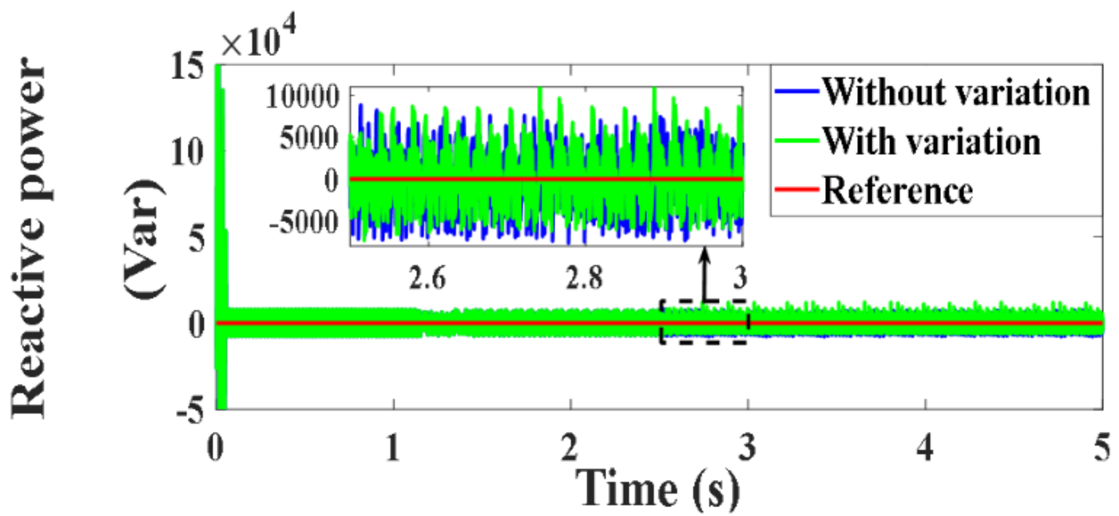
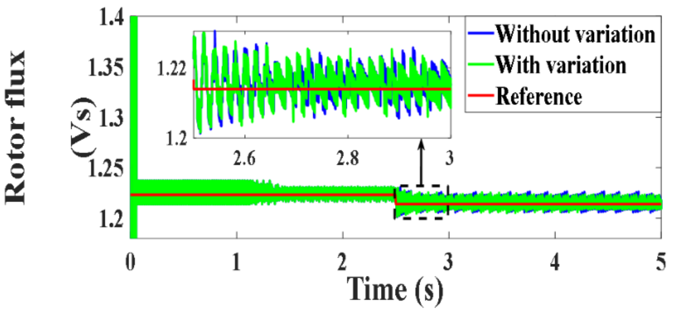
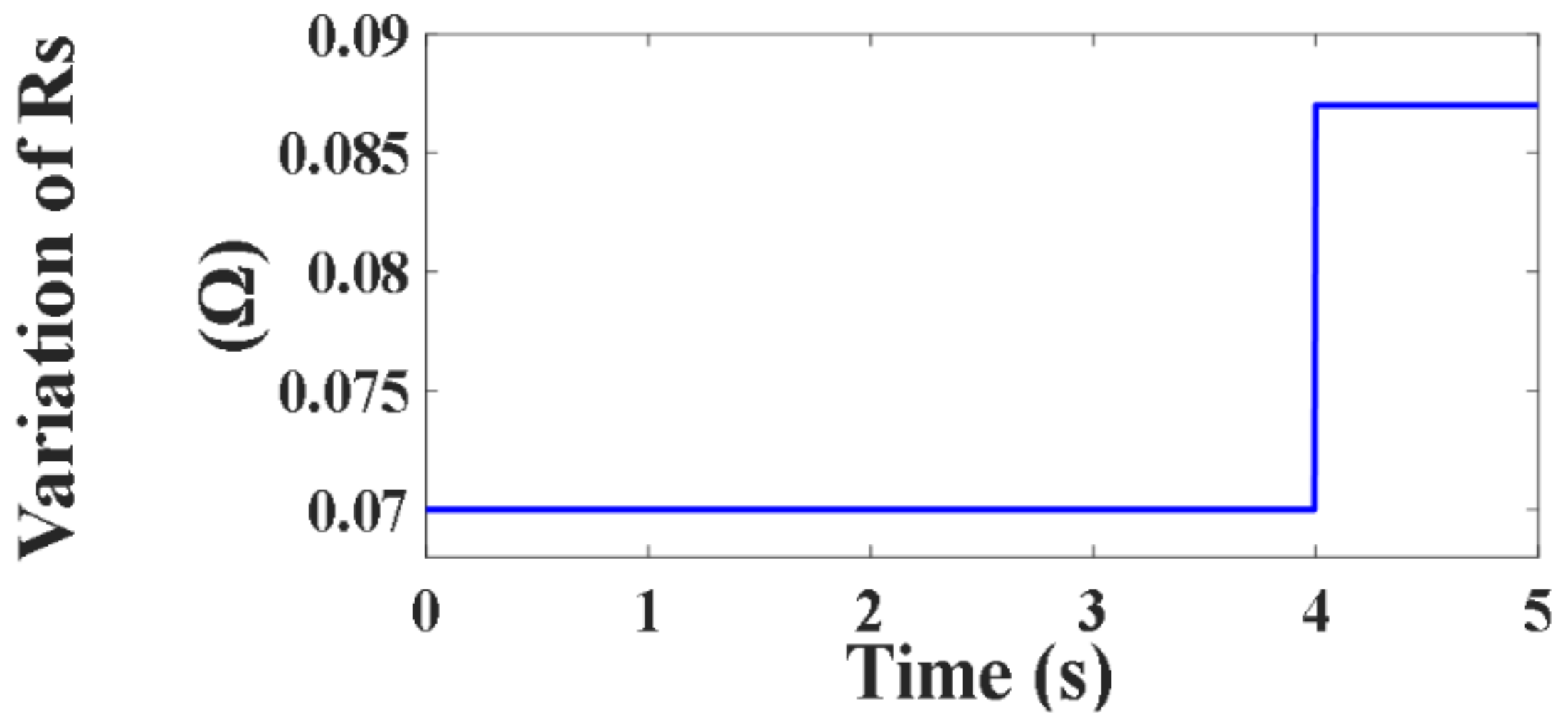
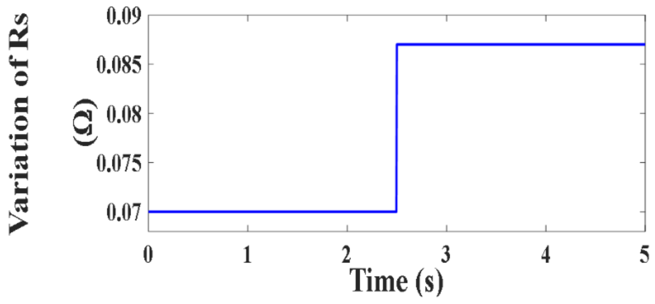
4.5. Testing under Proposed PVC with Parameter Variation

In this section, a robustness test for the proposed PVC and another control scheme recently introduced in [55,56,57,58] which adopts a similar operation mechanism is introduced. The purpose of this is to visualize the superiority of the proposed PVC in terms of system robustness.

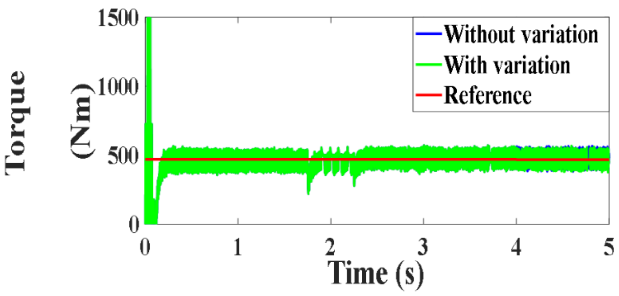
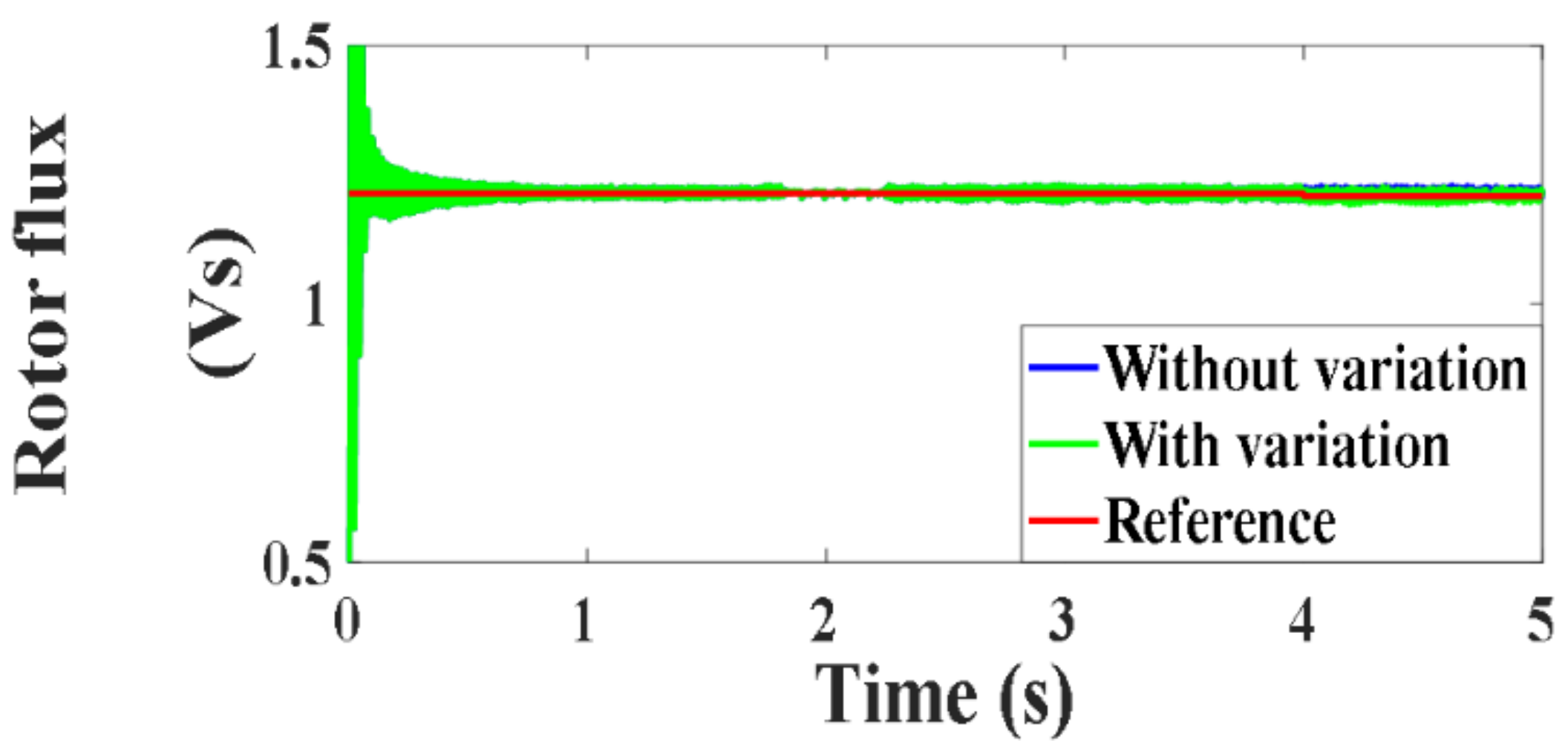
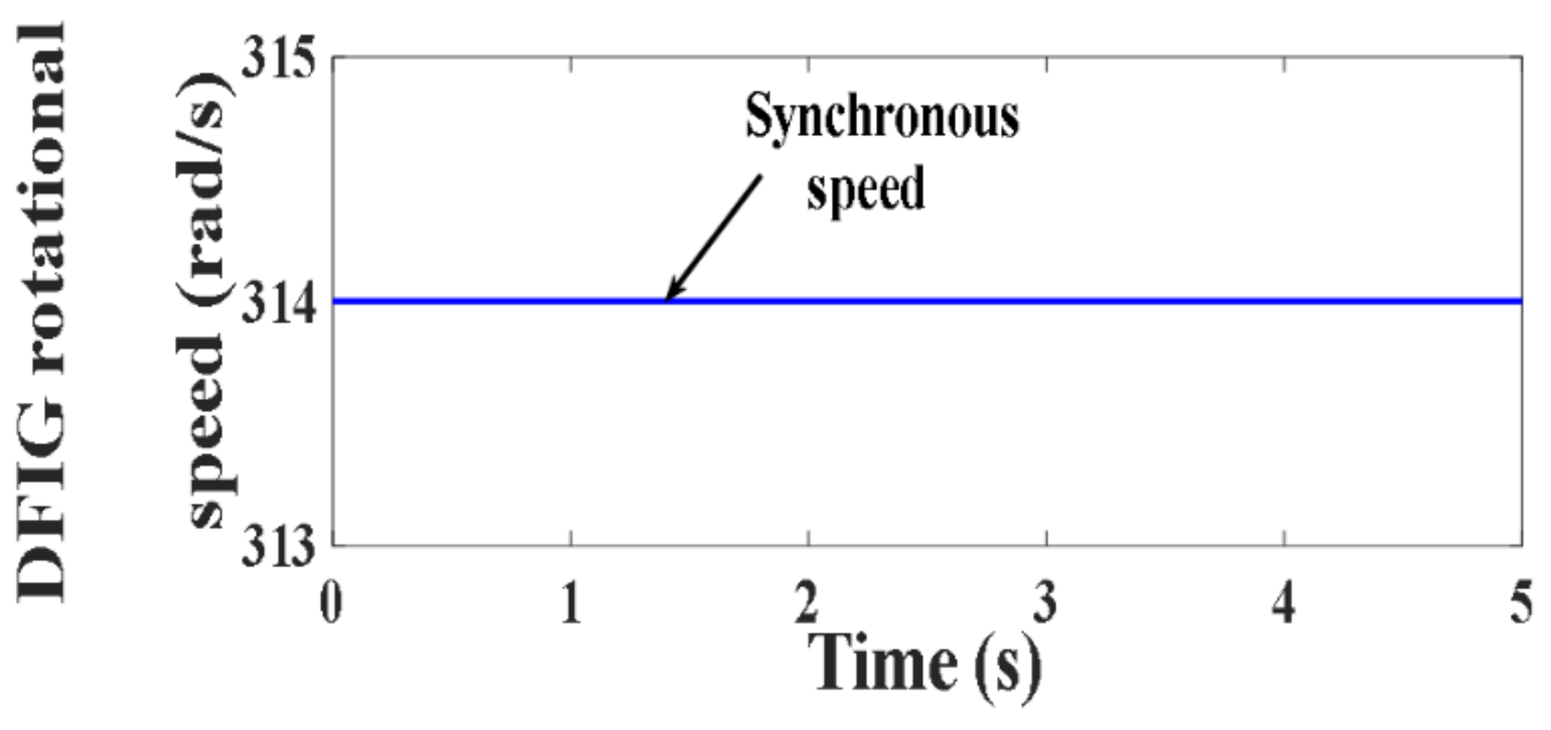
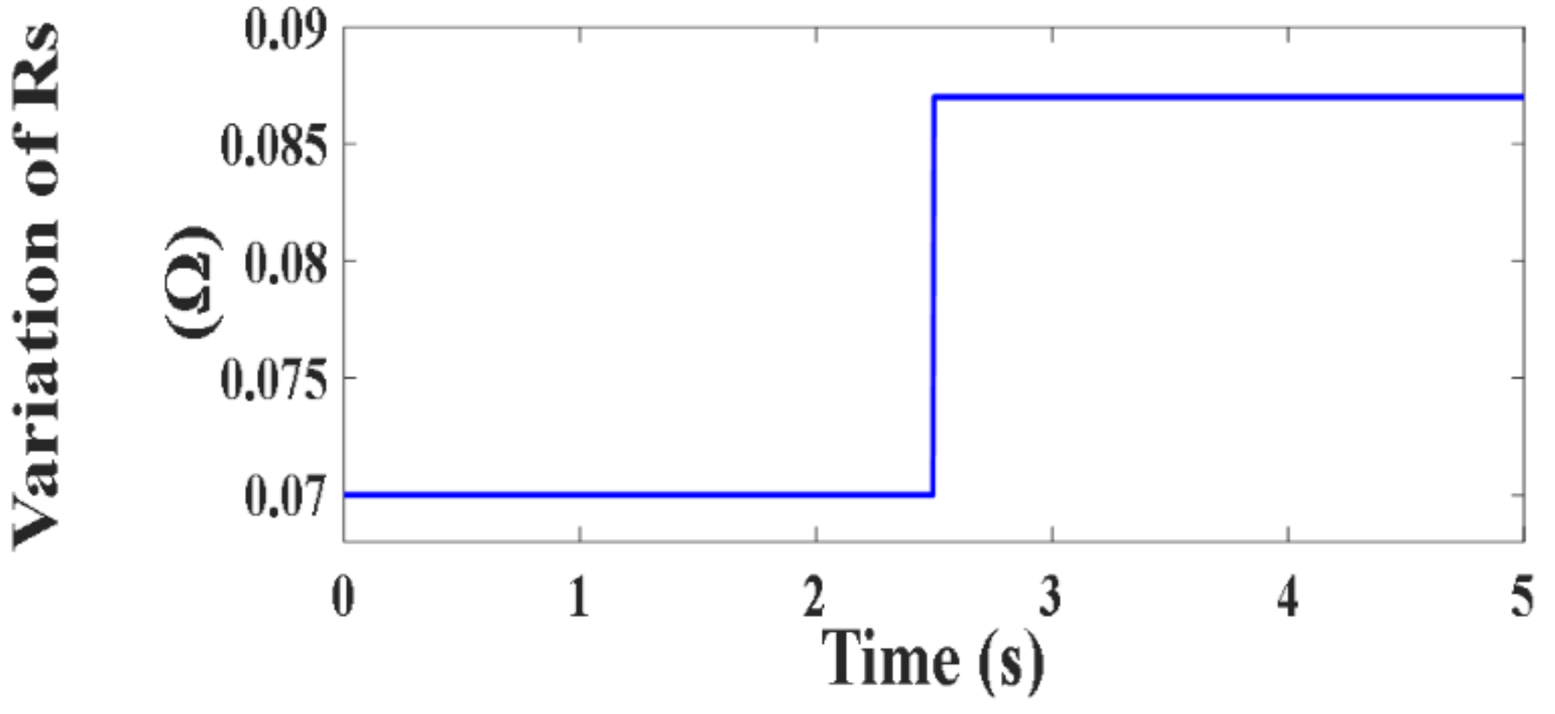
4.5.1. Testing under Proposed PVC with 20% Variation of R_s

In order to visualize the performance of the designed PVC under parameter mismatch, the following tests were performed. For the variable speed operation shown in Figure 65, a mismatch in stator resistance of 20% was applied at time t = 4 s (Figure 66). The obtained results reveal that the designed PVC succeeded in maintaining the proper operation under the resistance variation. This was confirmed by the maintained actual values of active and reactive powers, torque and rotor flux (Figure 67, Figure 68, Figure 69 and Figure 70) for variable speed operation. The same robust behavior is also maintained for fixed speed operation (Figure 71) under a resistance variation of 20% applied at time t = 2.5 s (Figure 72). The obtained results for active and reactive powers (Figure 73 and Figure 74) and for torque, and rotor flux (Figure 75 and Figure 76) are confirming the robust dynamic behavior of the DFIG.

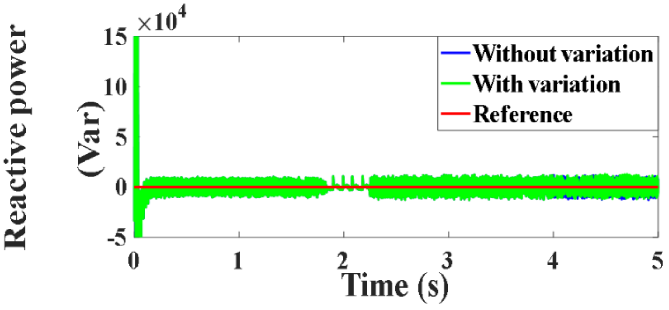
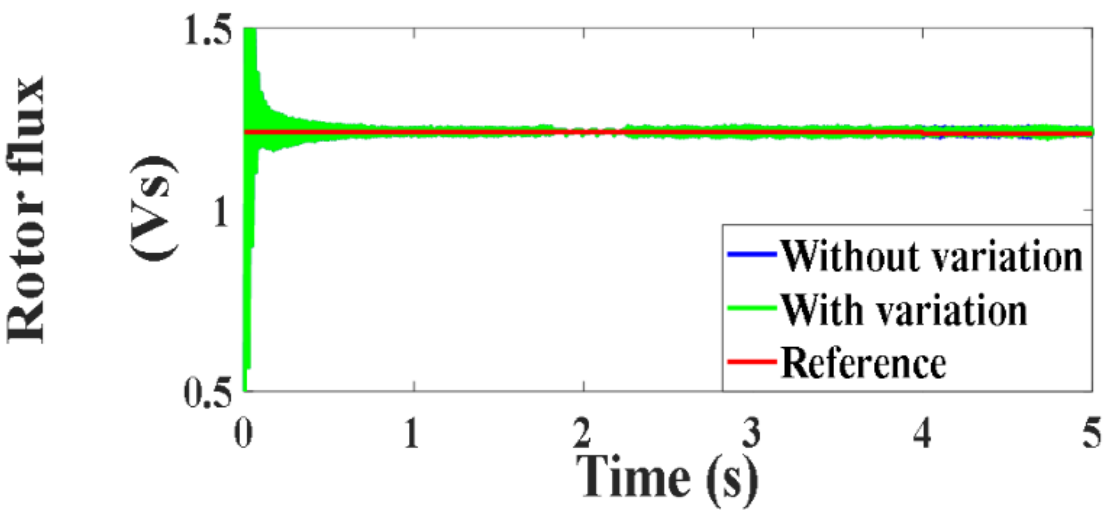
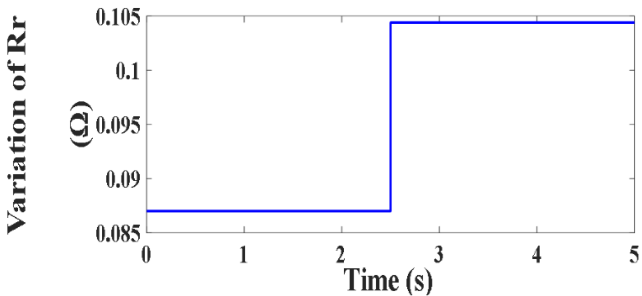
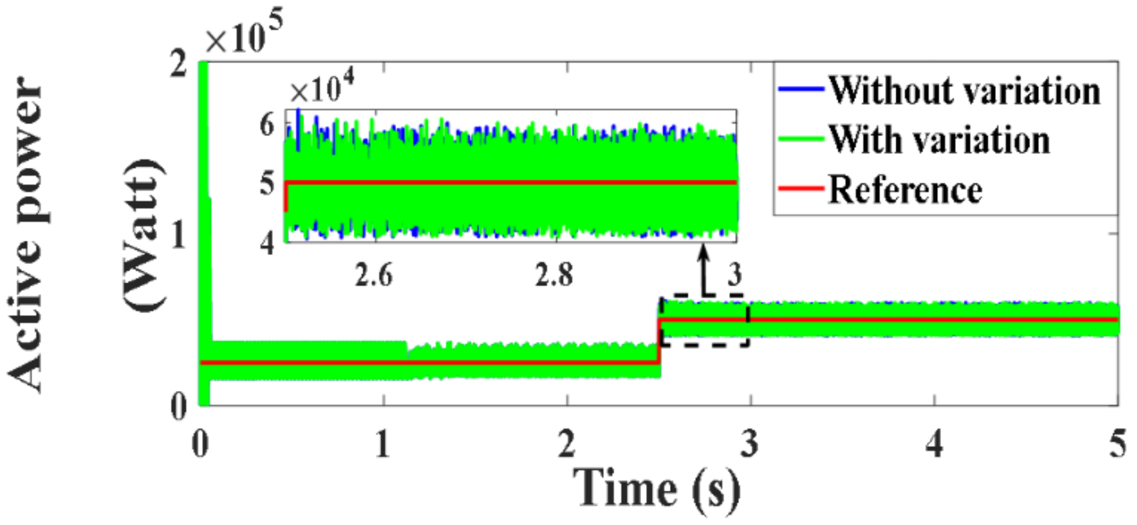
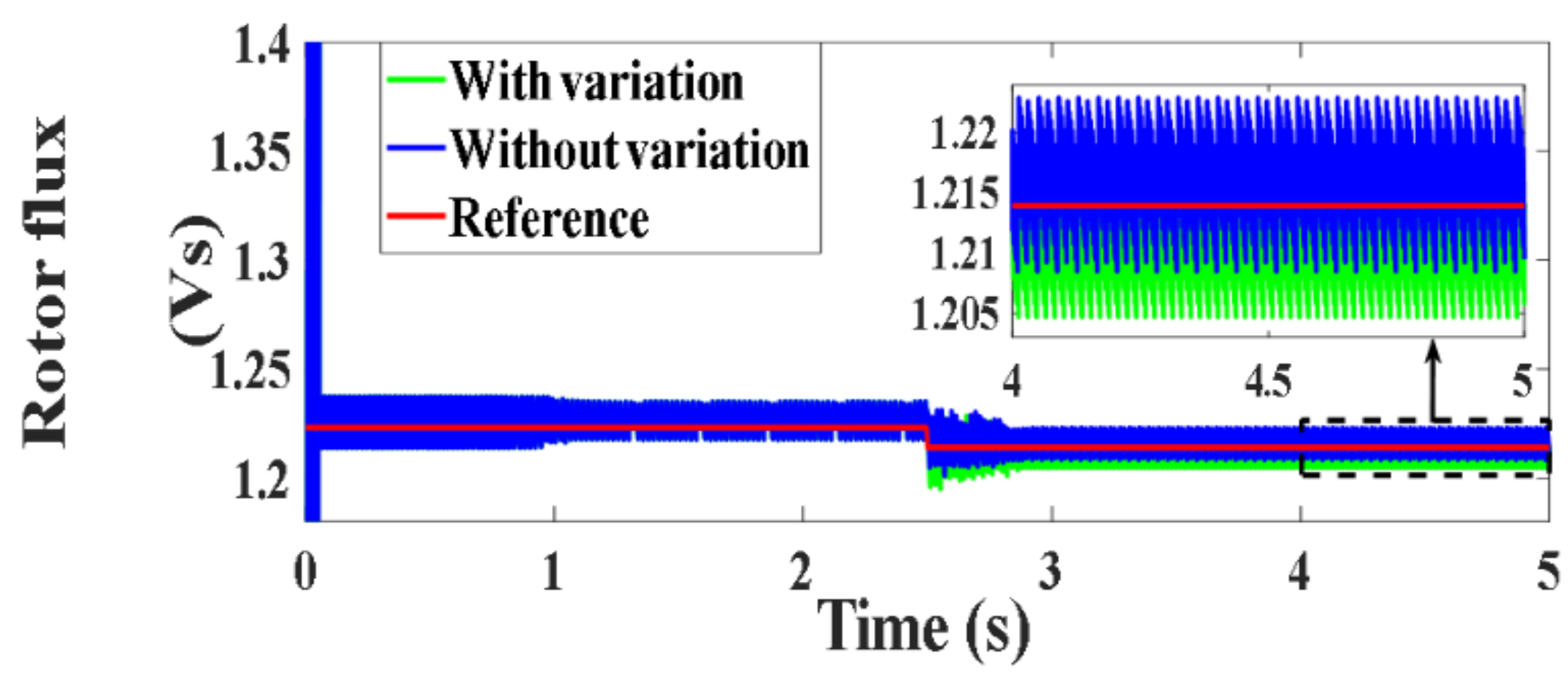
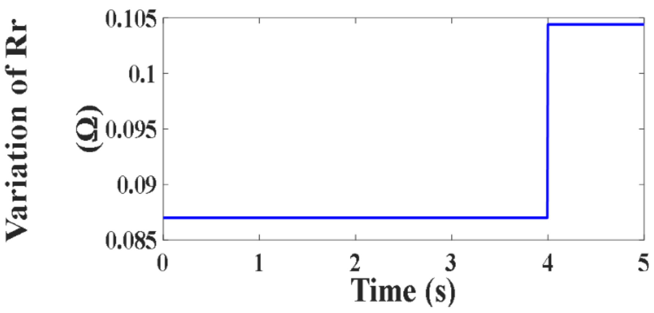
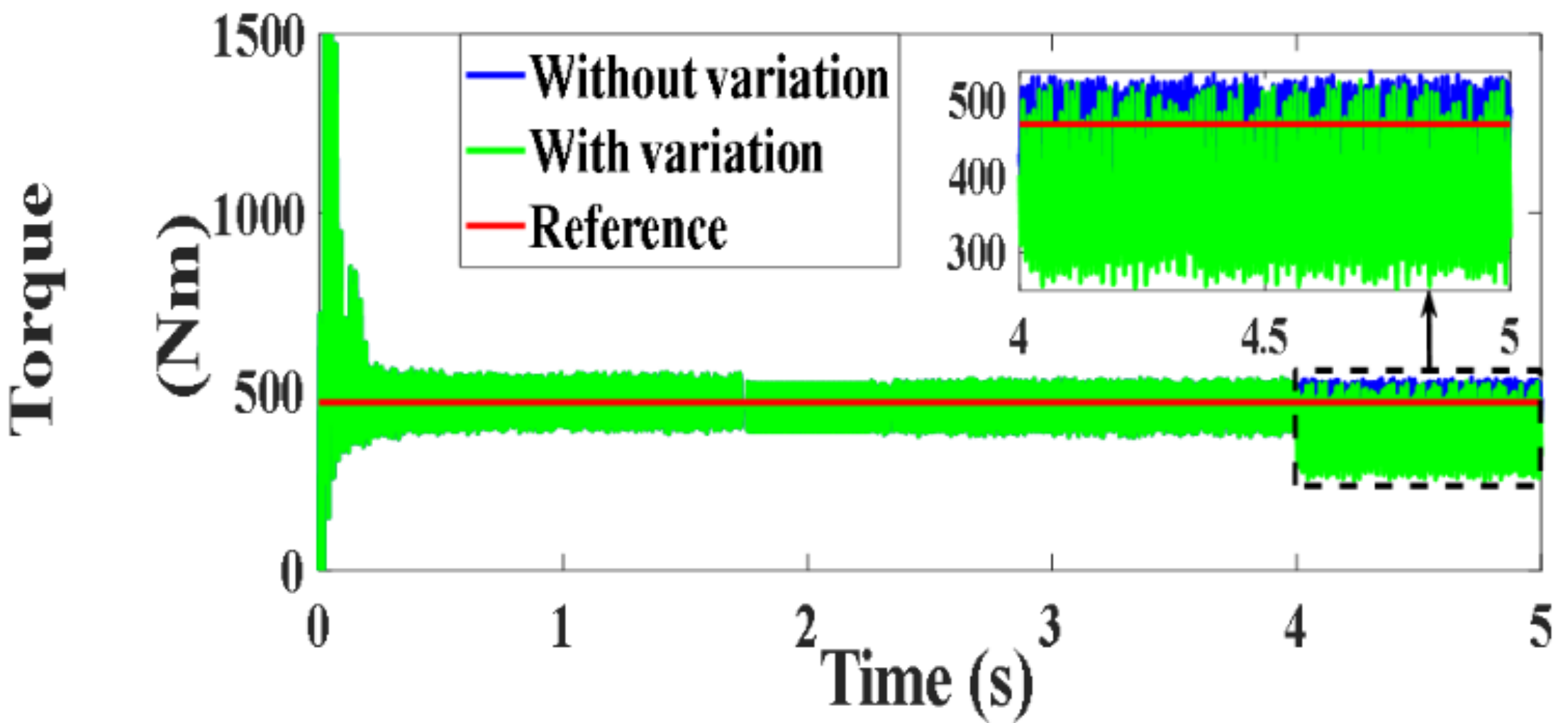
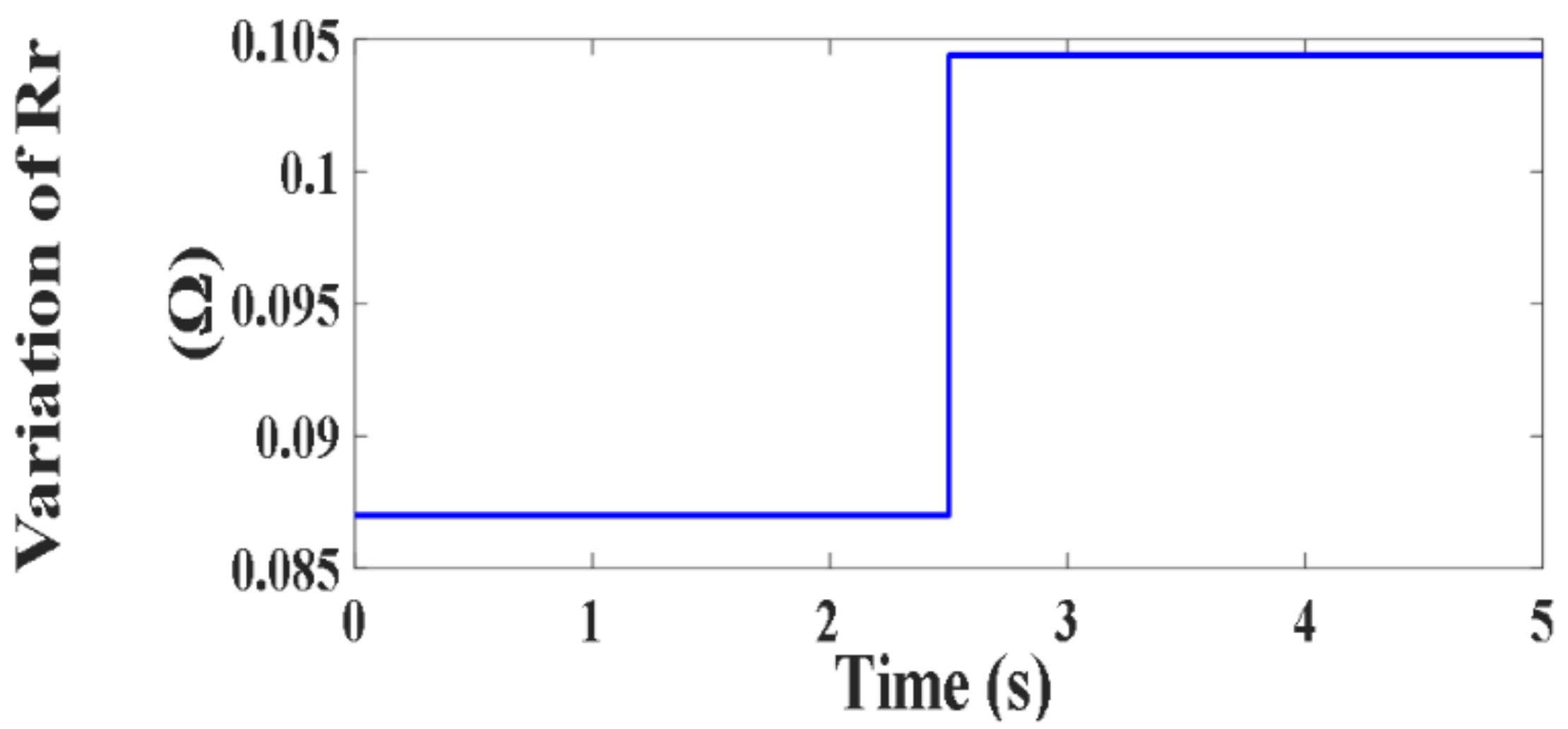
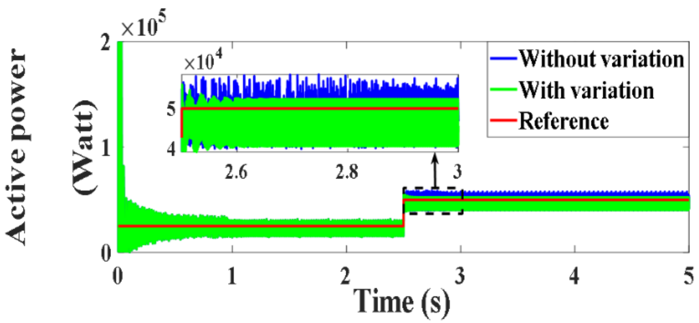
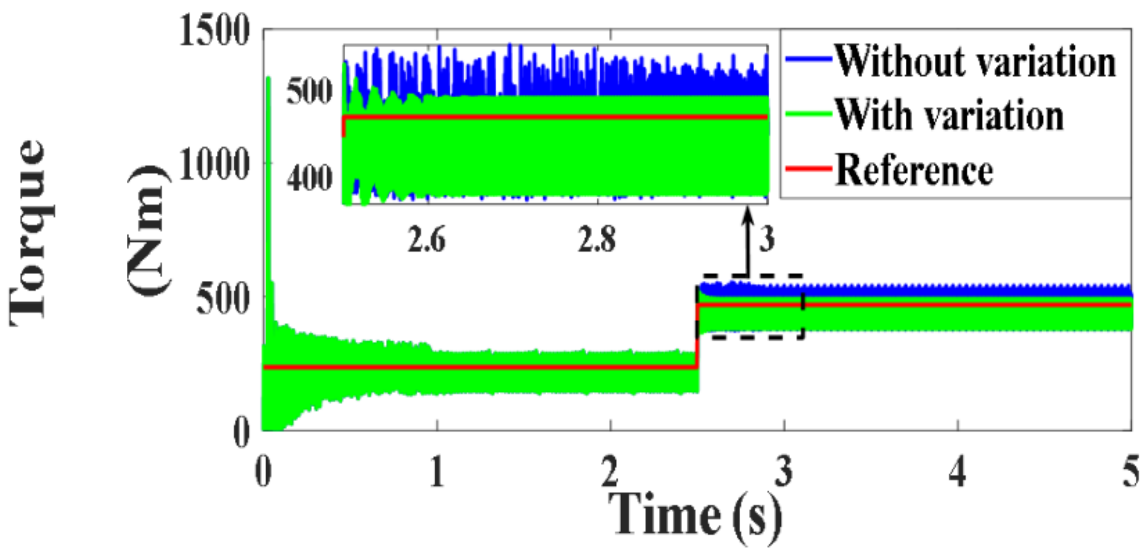
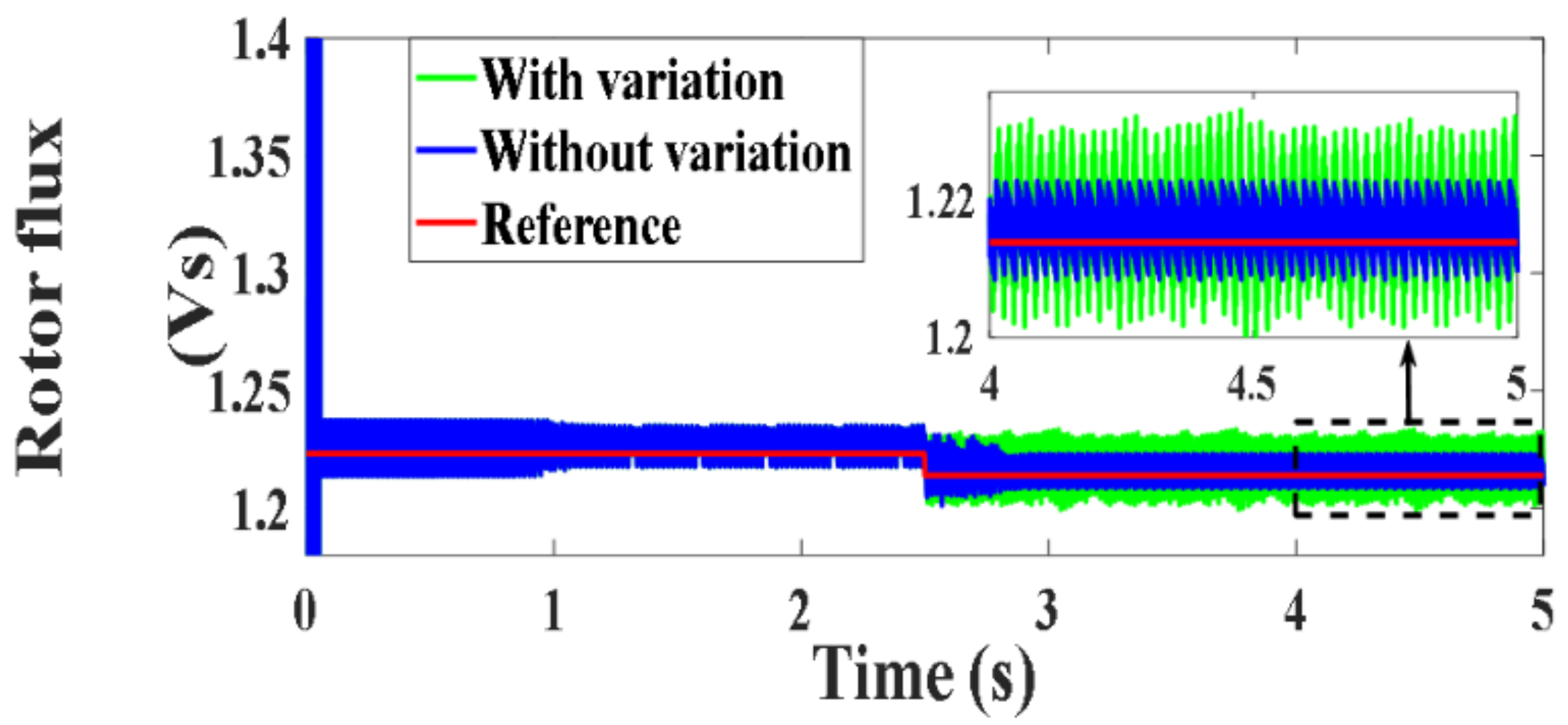
4.5.2. Testing under Proposed PVC with 20% Variation of R_r

The second parameter variation was made with the rotor resistance value with an increase of 20%. The values of active and reactive powers, torque and rotor flux for variable wind speed shown in Figure 77 with R_s variation (Figure 78) are presented in Figure 79, Figure 80, Figure 81 and Figure 82, respectively. Similarly, for the fixed speed operation (Figure 83) with R_s variation (Figure 84), the results are illustrated for the same variables in Figure 85, Figure 86, Figure 87 and Figure 88, respectively. The obtained results present an adequate performance under the resistance variation, which again confirms the robustness of the designed PVC scheme.

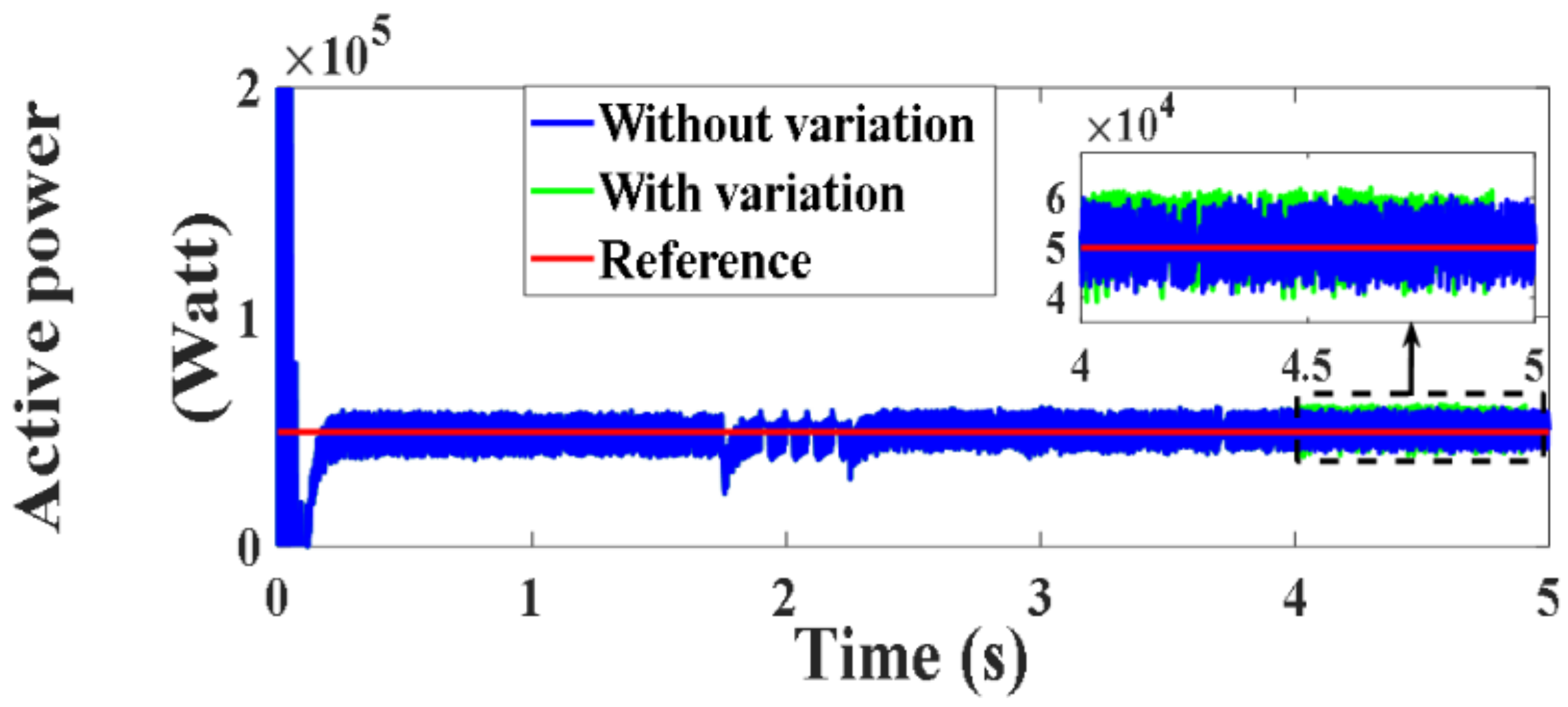
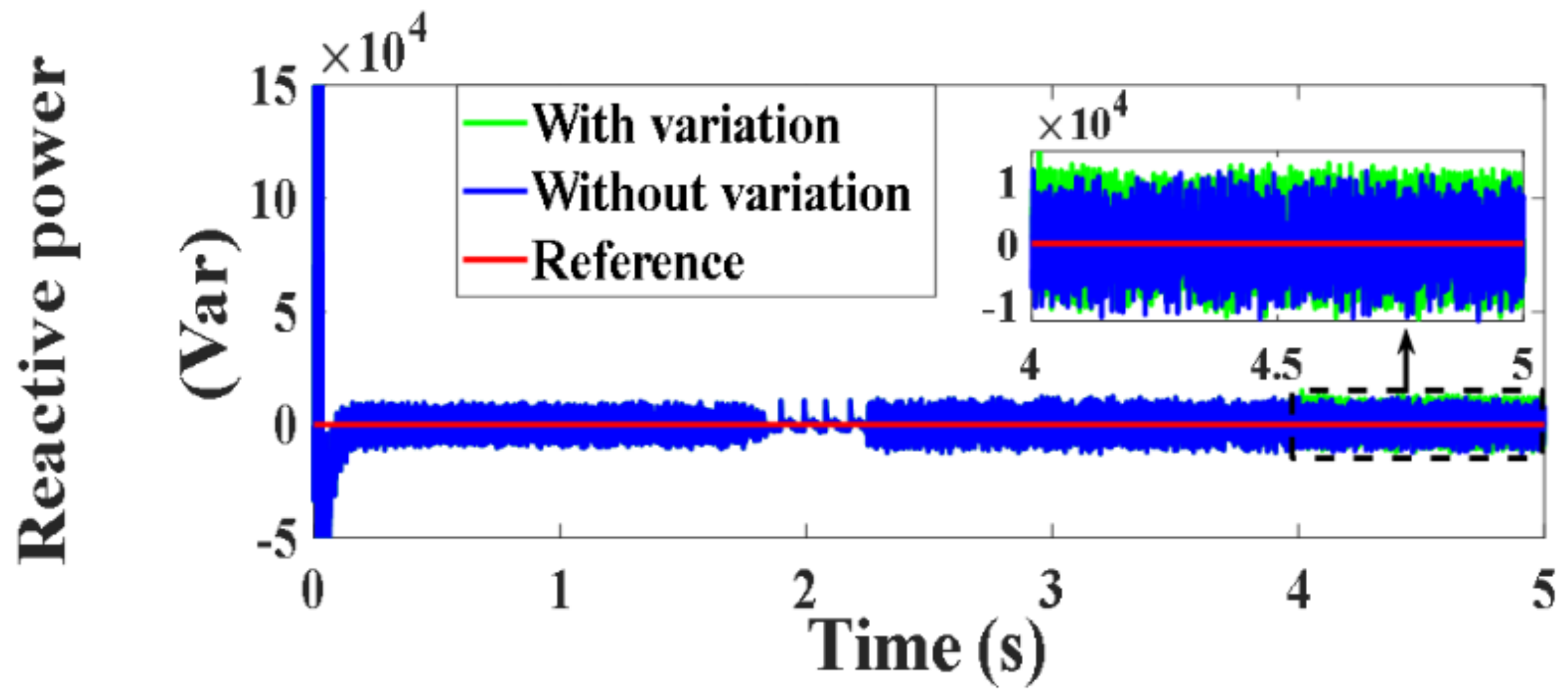
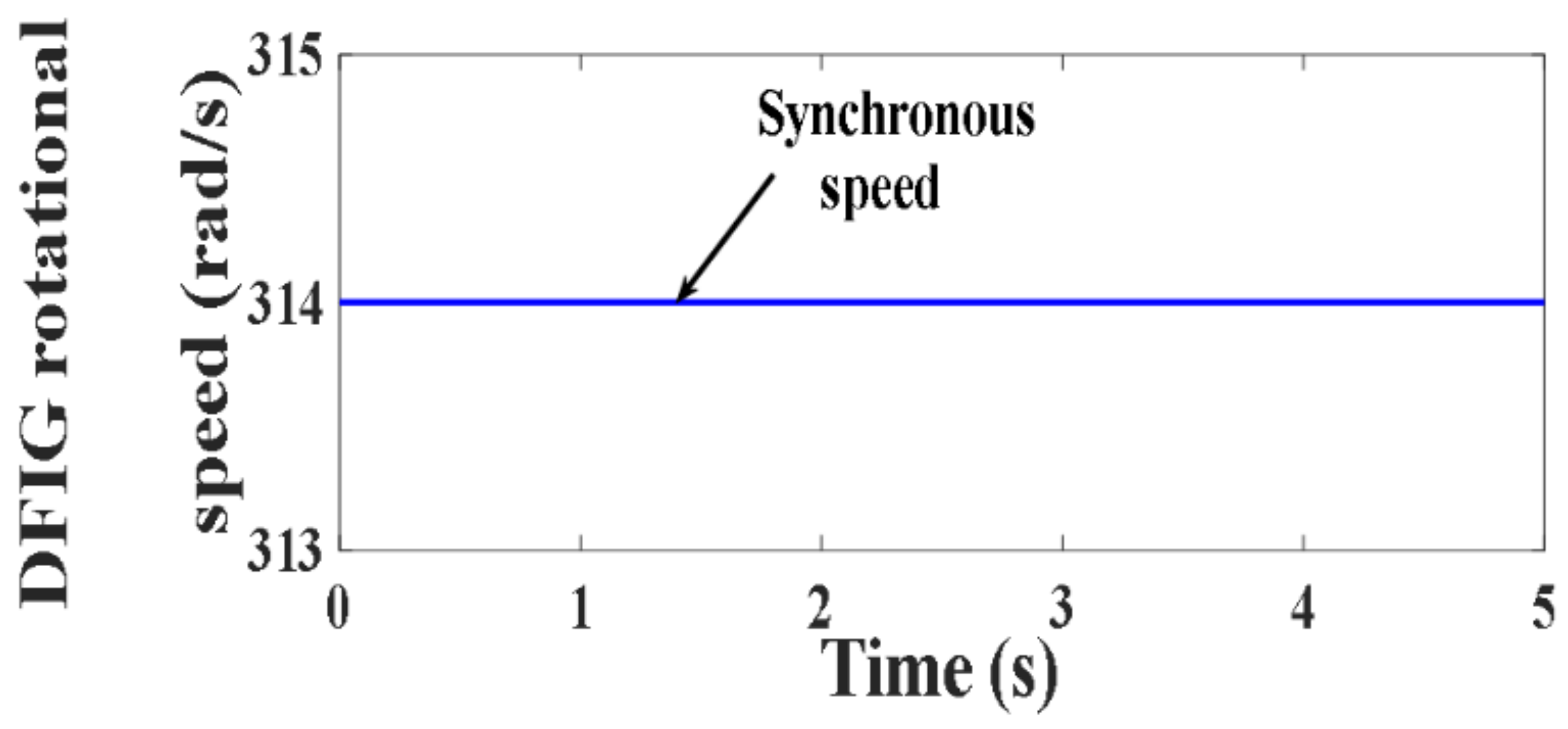
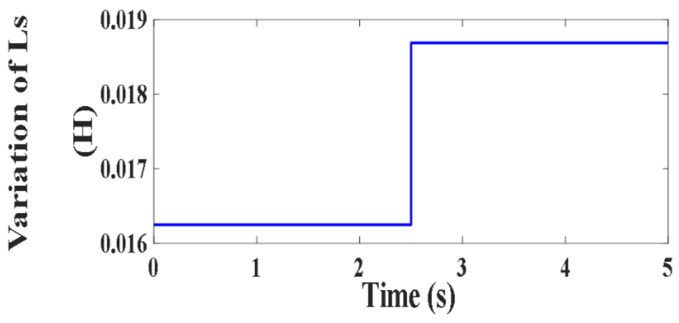
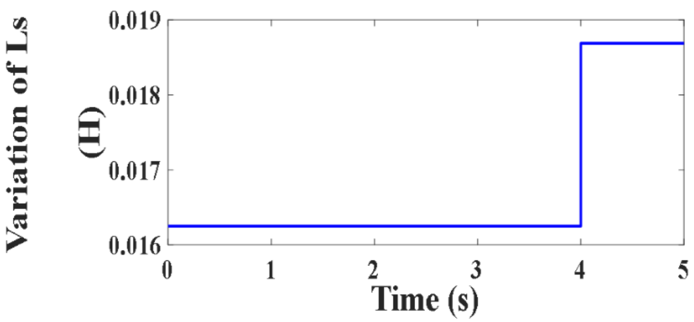
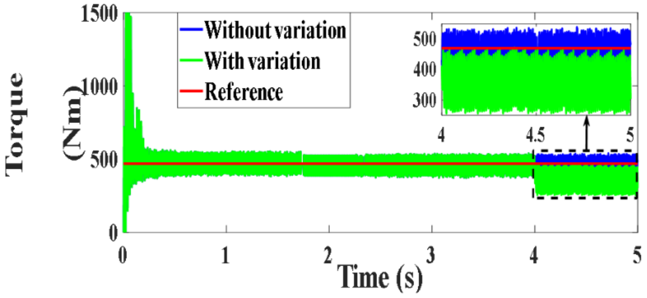
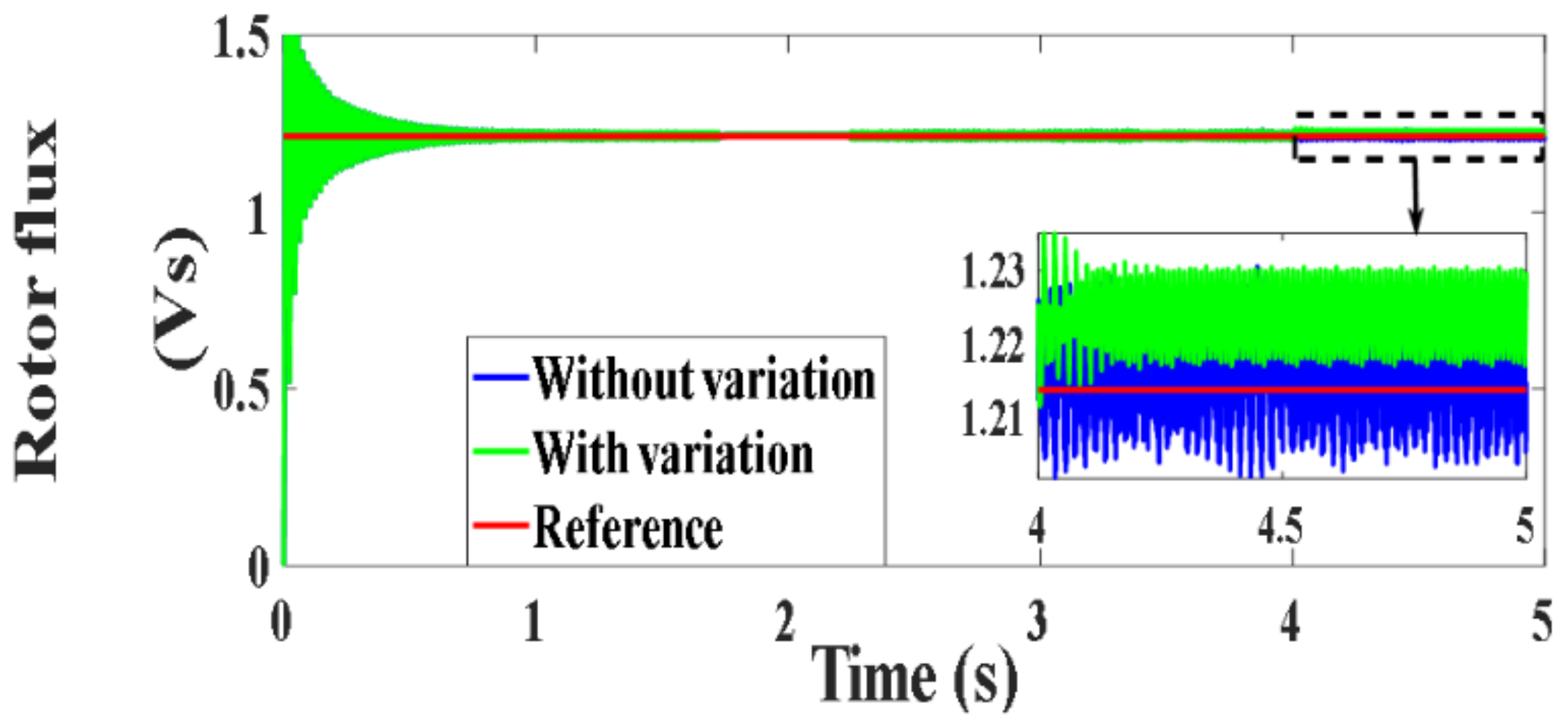
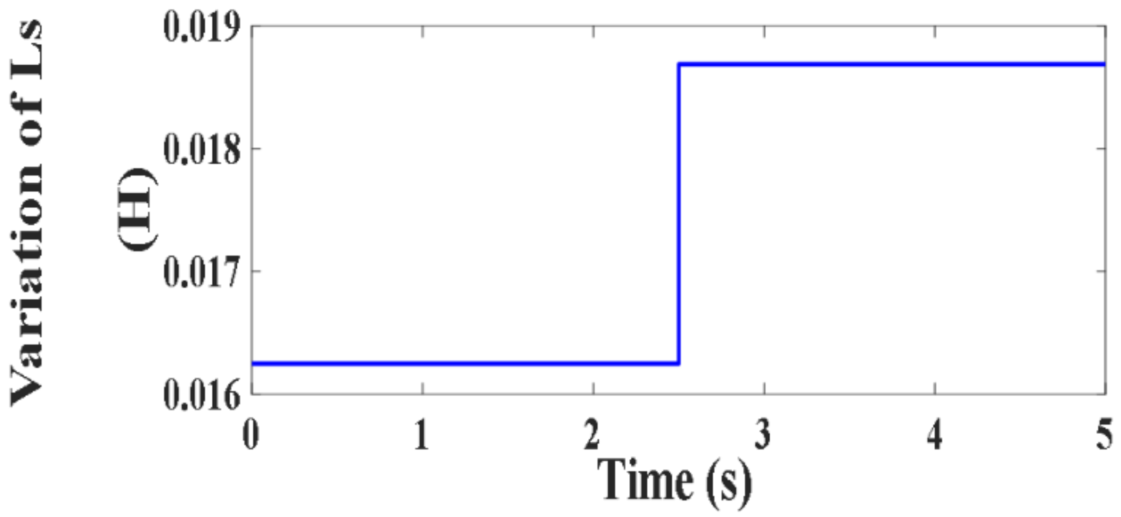
4.5.3. Testing under Proposed PVC with 15% Variation of L_s

The performance of the DFIG under PVC was also tested for the variable speed operation (Figure 89) while considering a mismatch of 15% in the stator inductance (L_s) value (Figure 90). The obtained results for the active and reactive powers, torque and rotor flux are presented in Figure 91, Figure 92, Figure 93 and Figure 94. A similar test is applied under the fixed speed operation (Figure 95) with a L_s variation (Figure 96), and the results are presented in Figure 97, Figure 98, Figure 99 and Figure 100, respectively. The obtained results reveal that the DFIG maintains an appropriate operation even under the inductance variation.

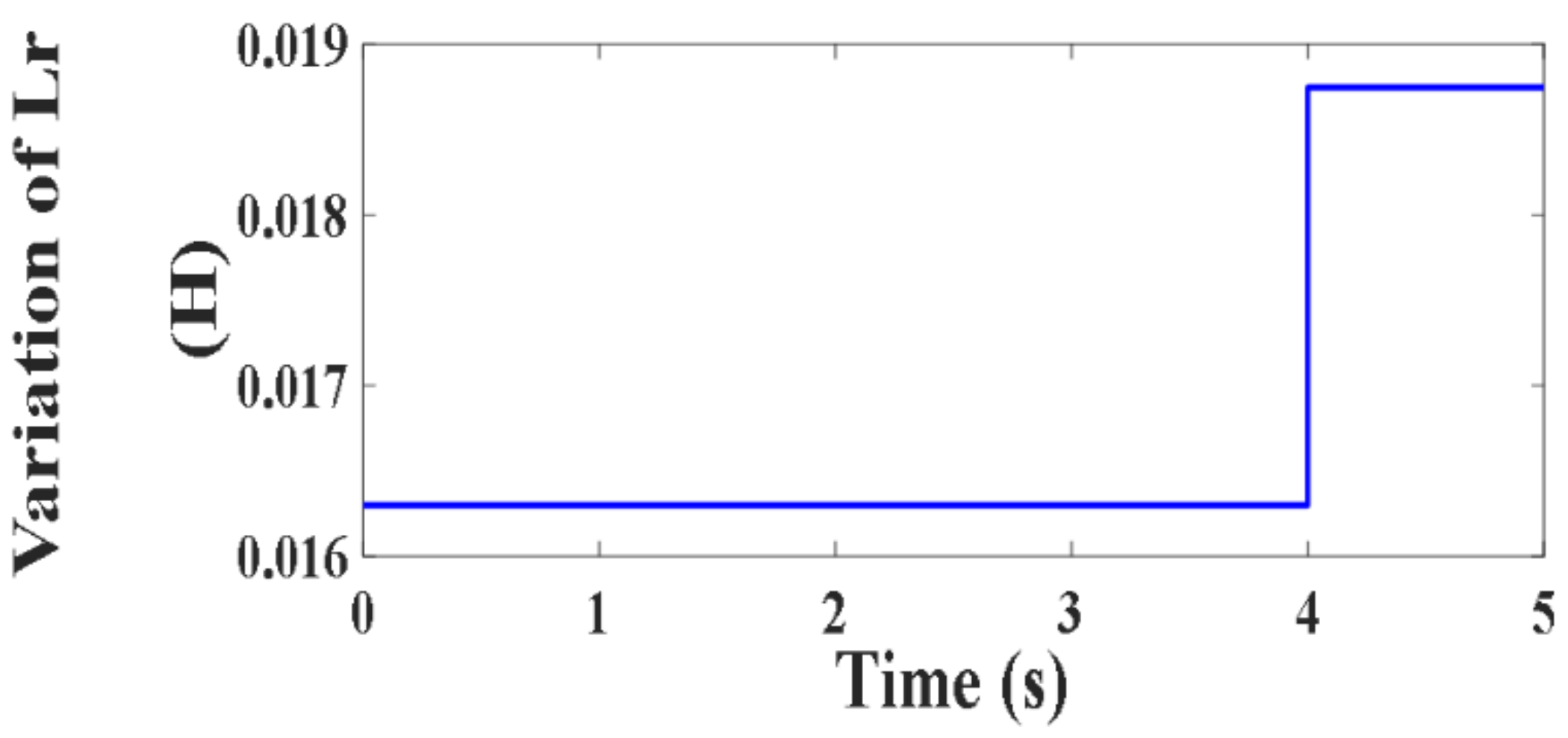
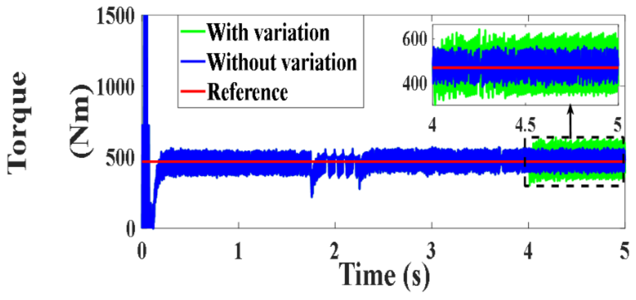
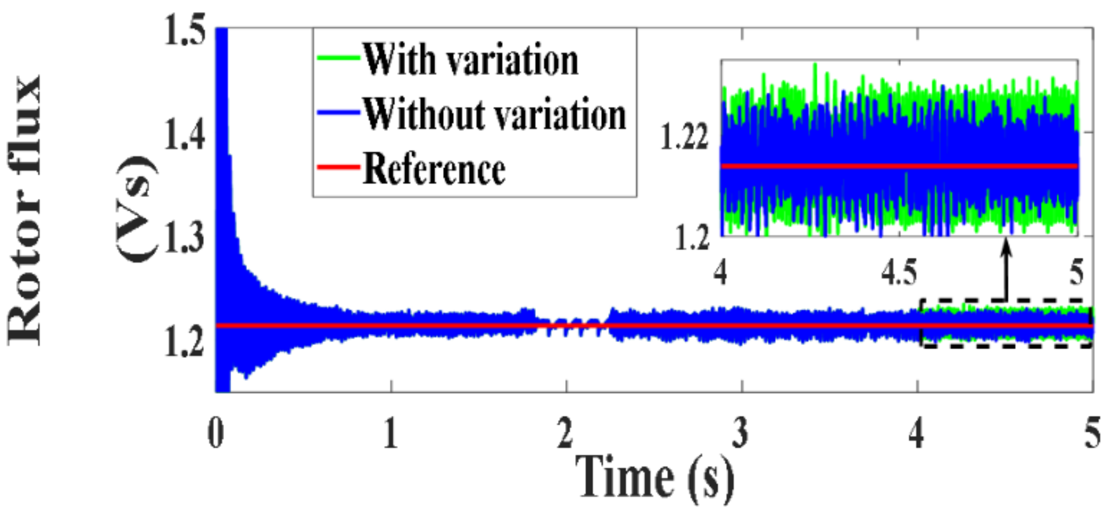
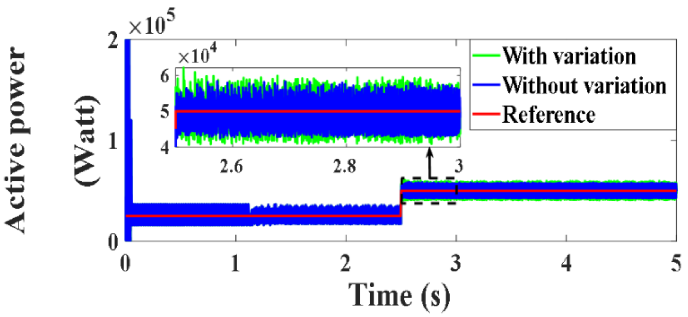
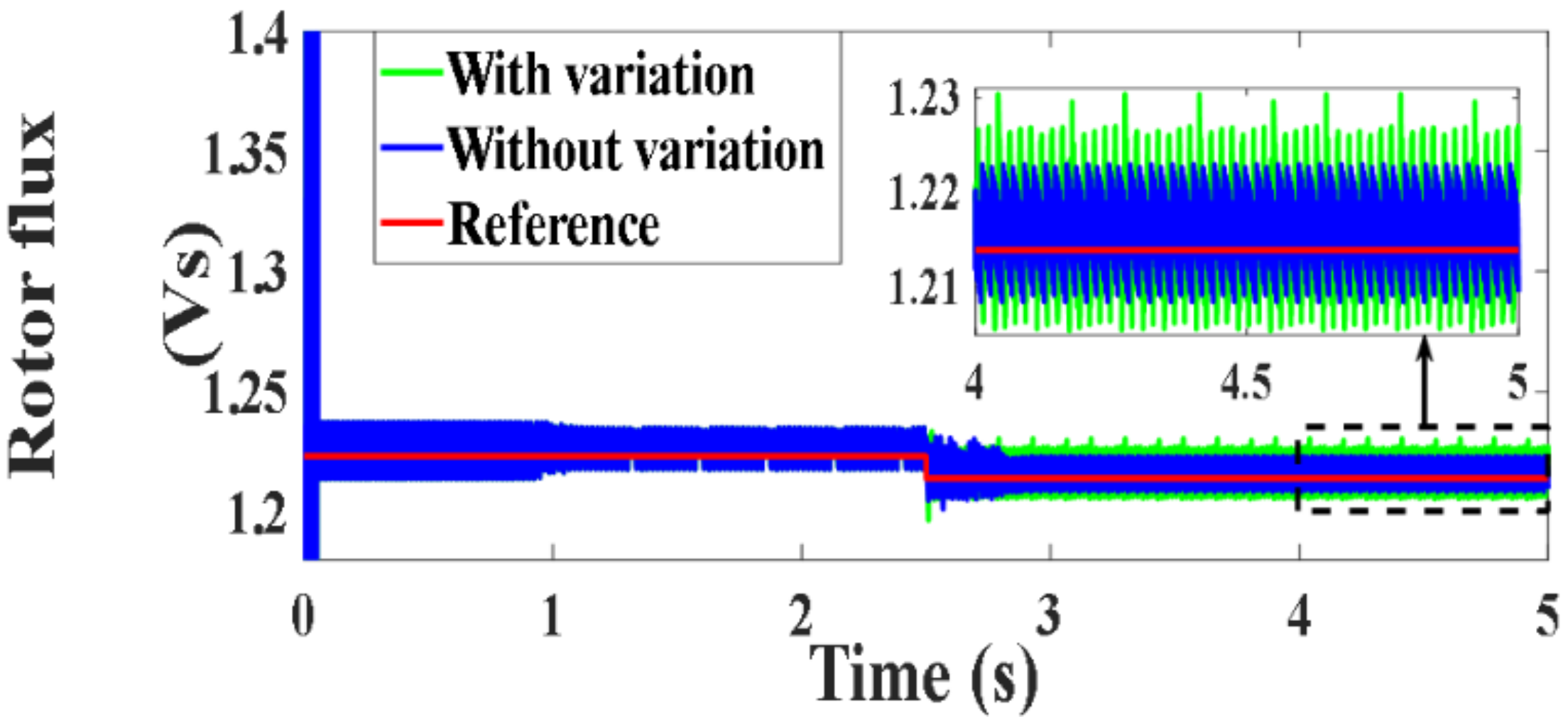
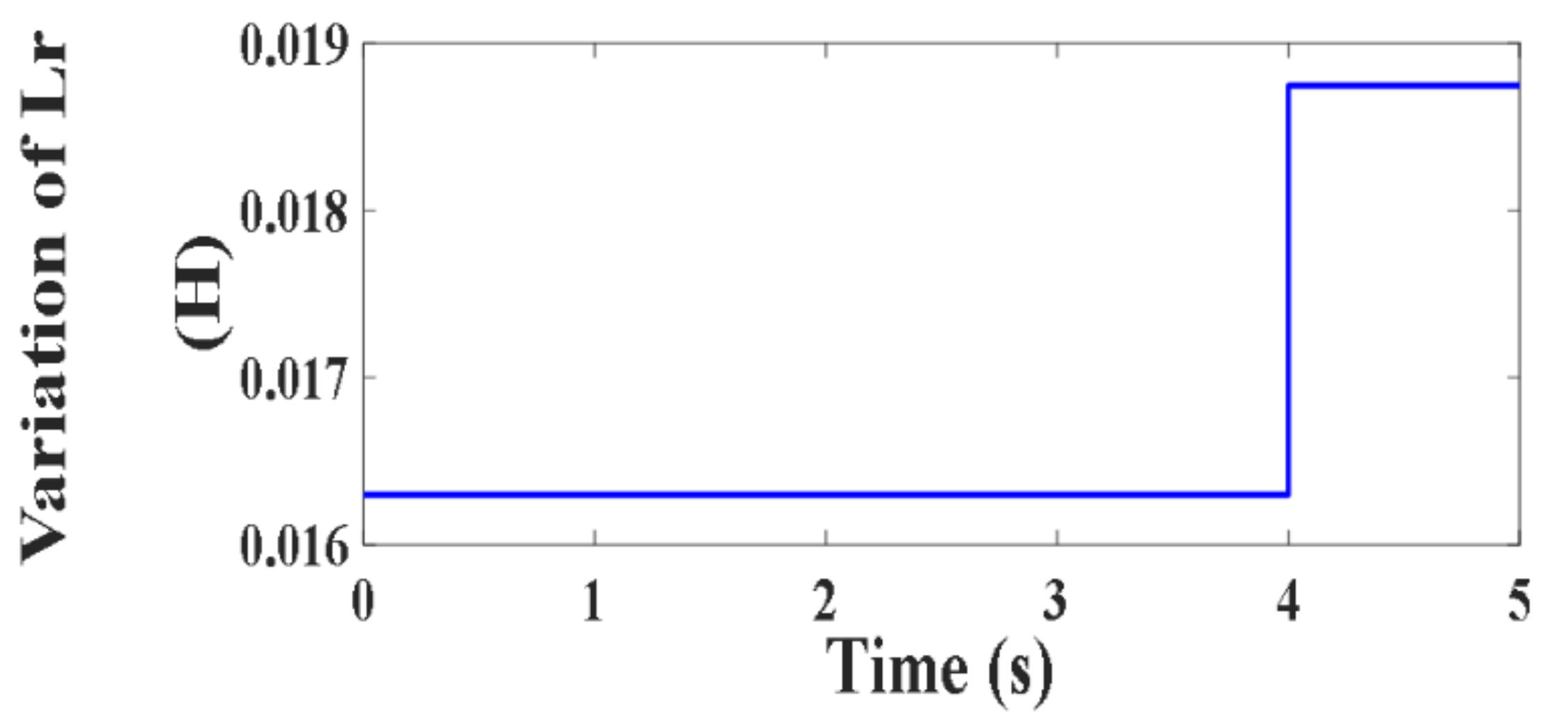
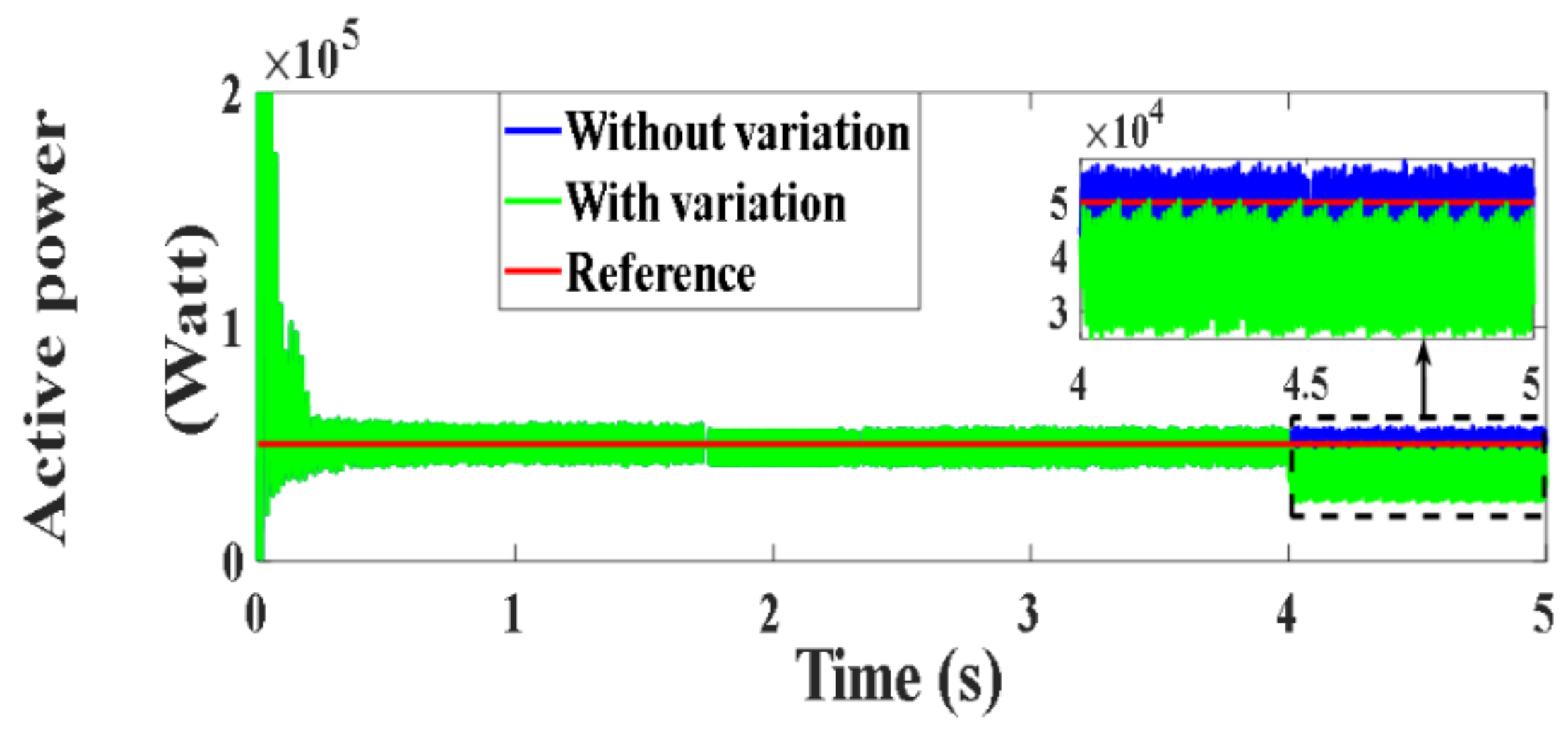
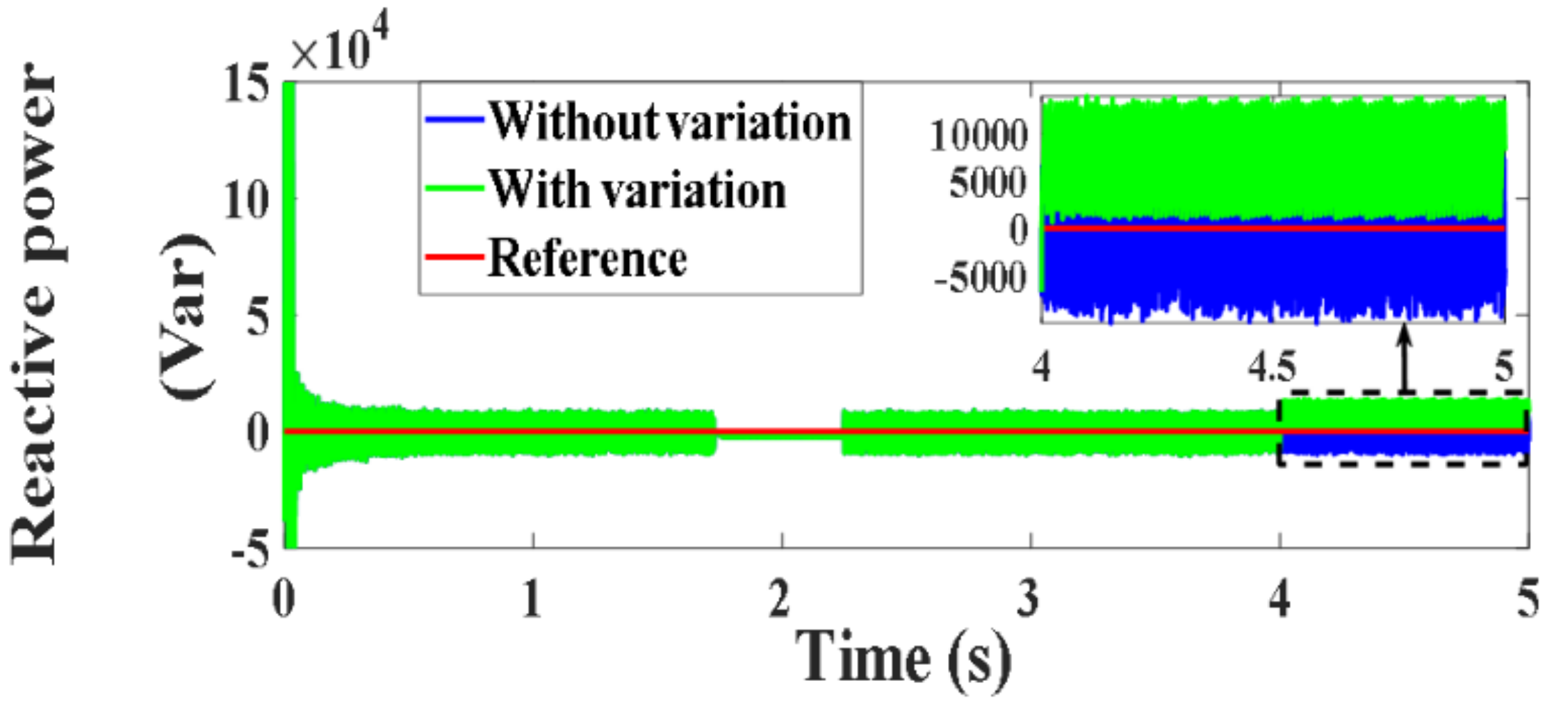
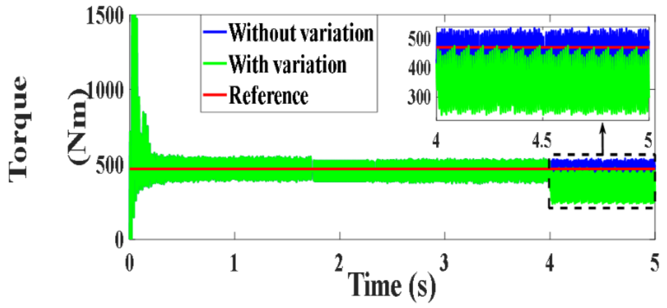
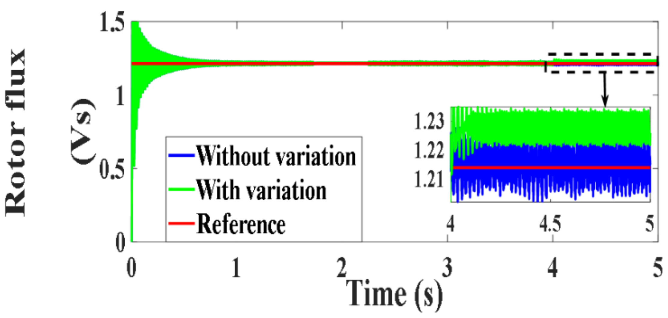
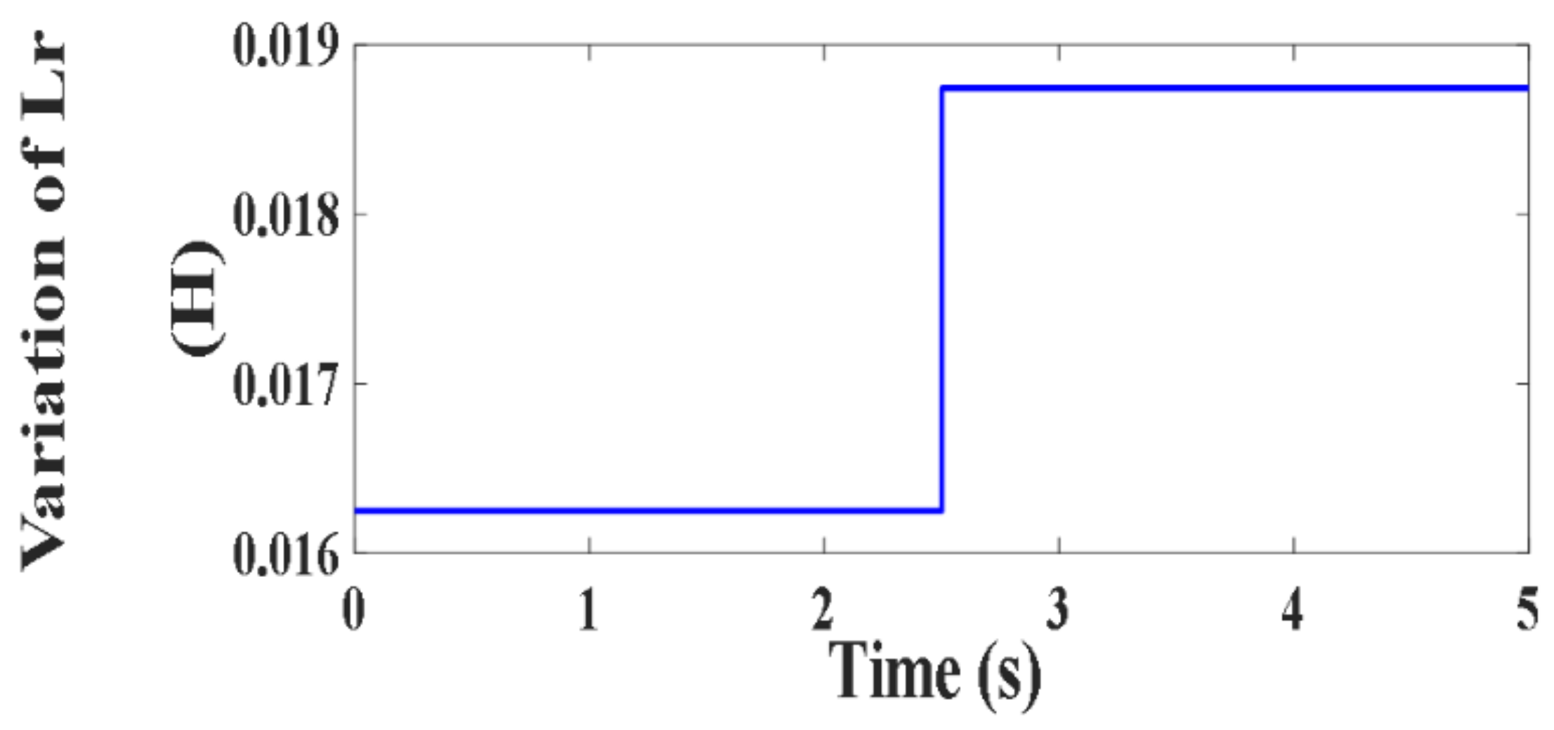
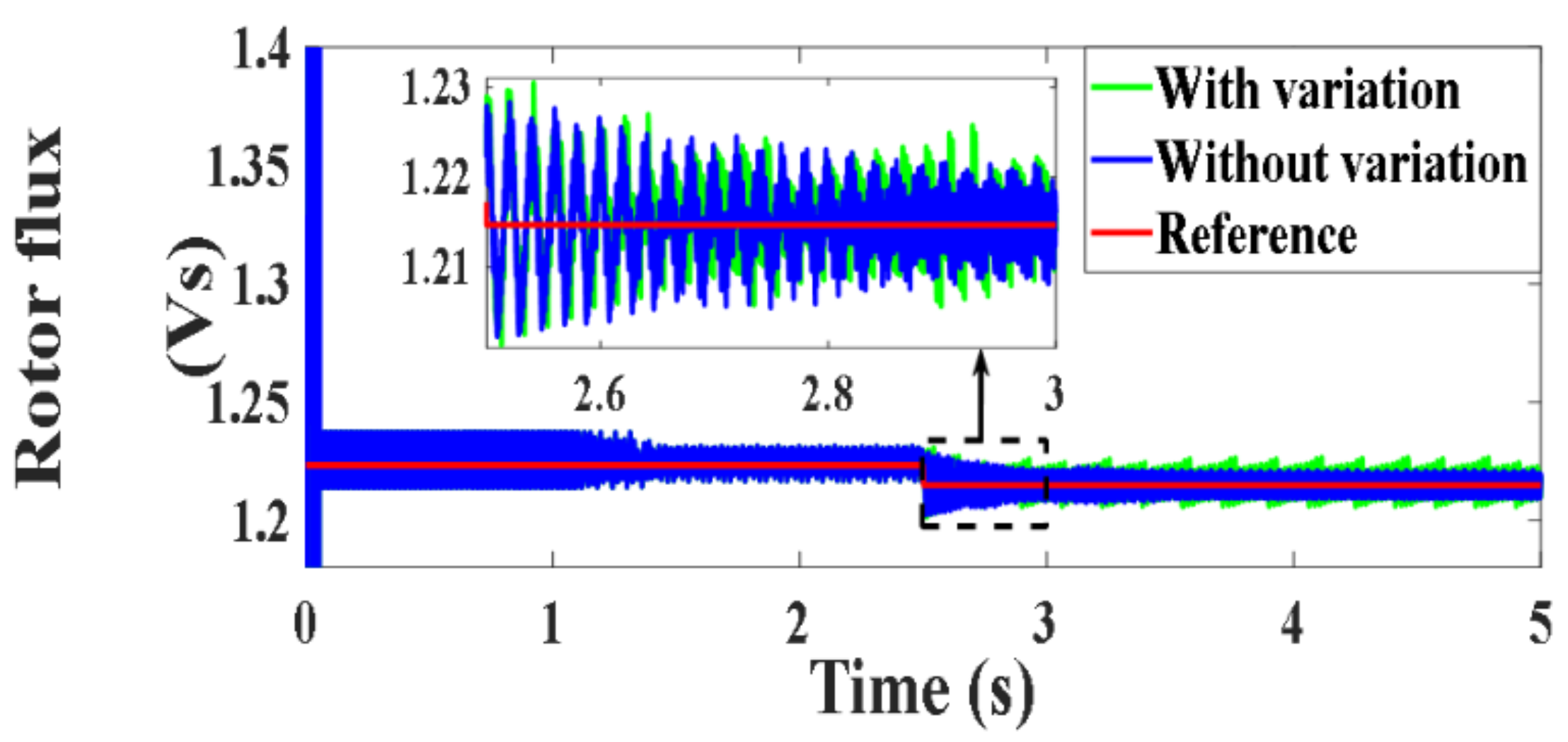
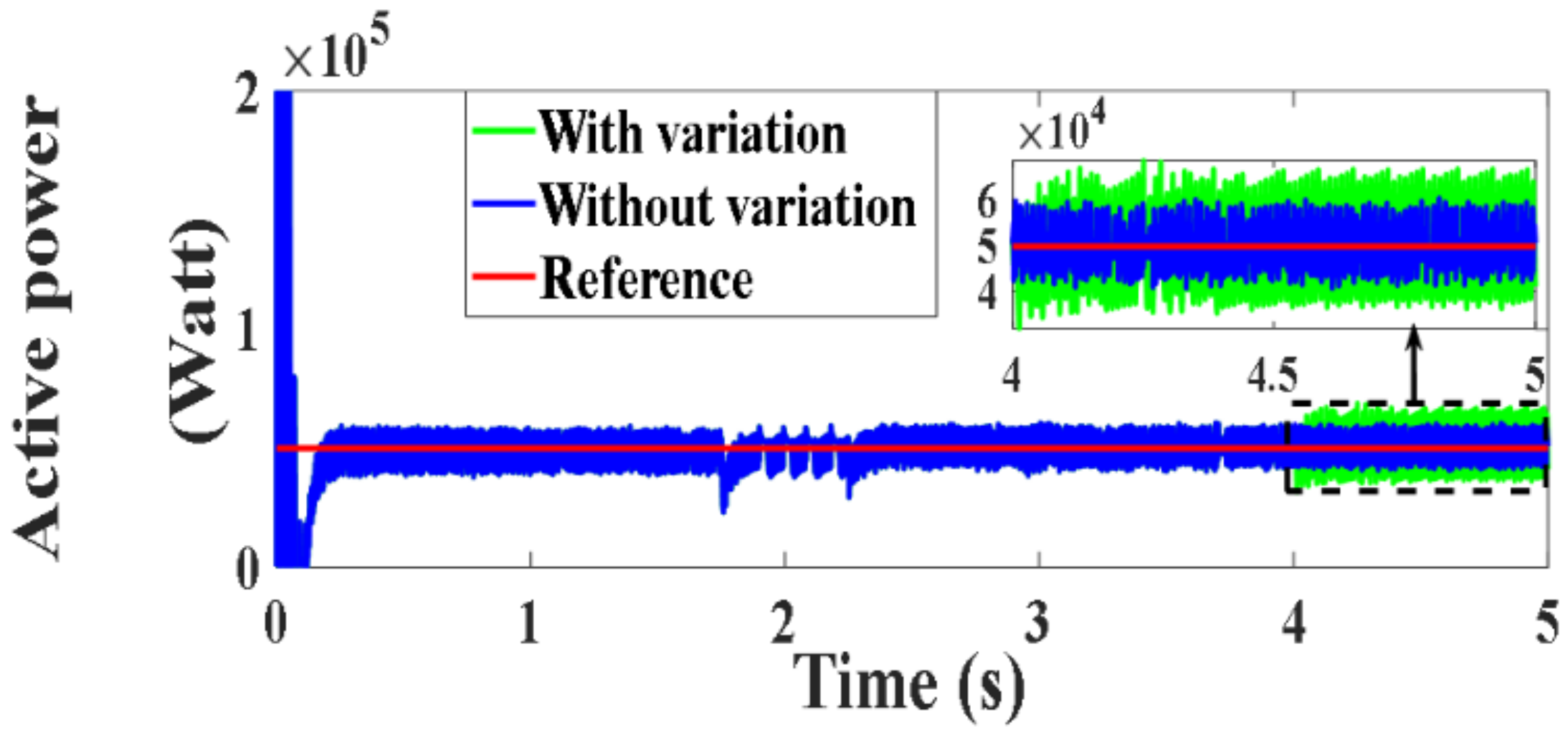
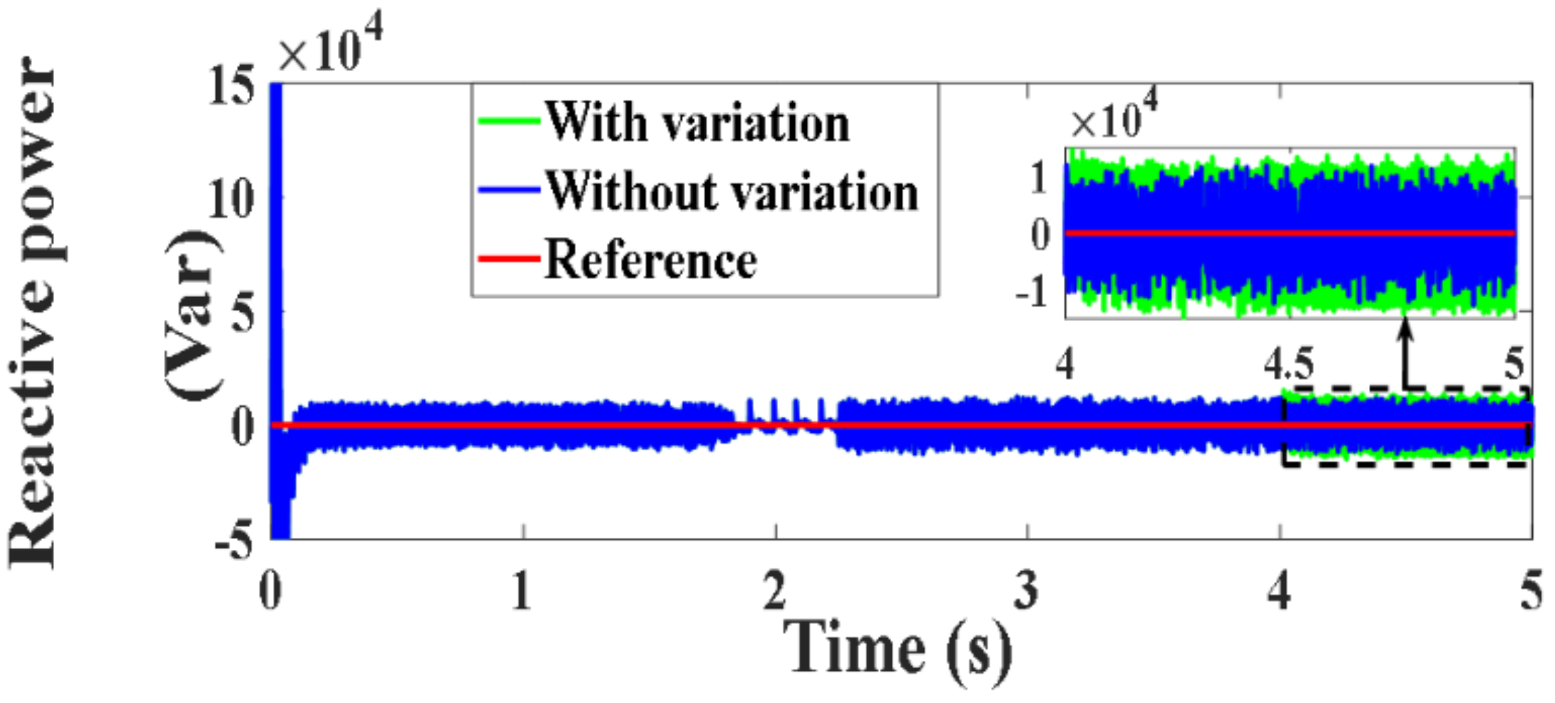
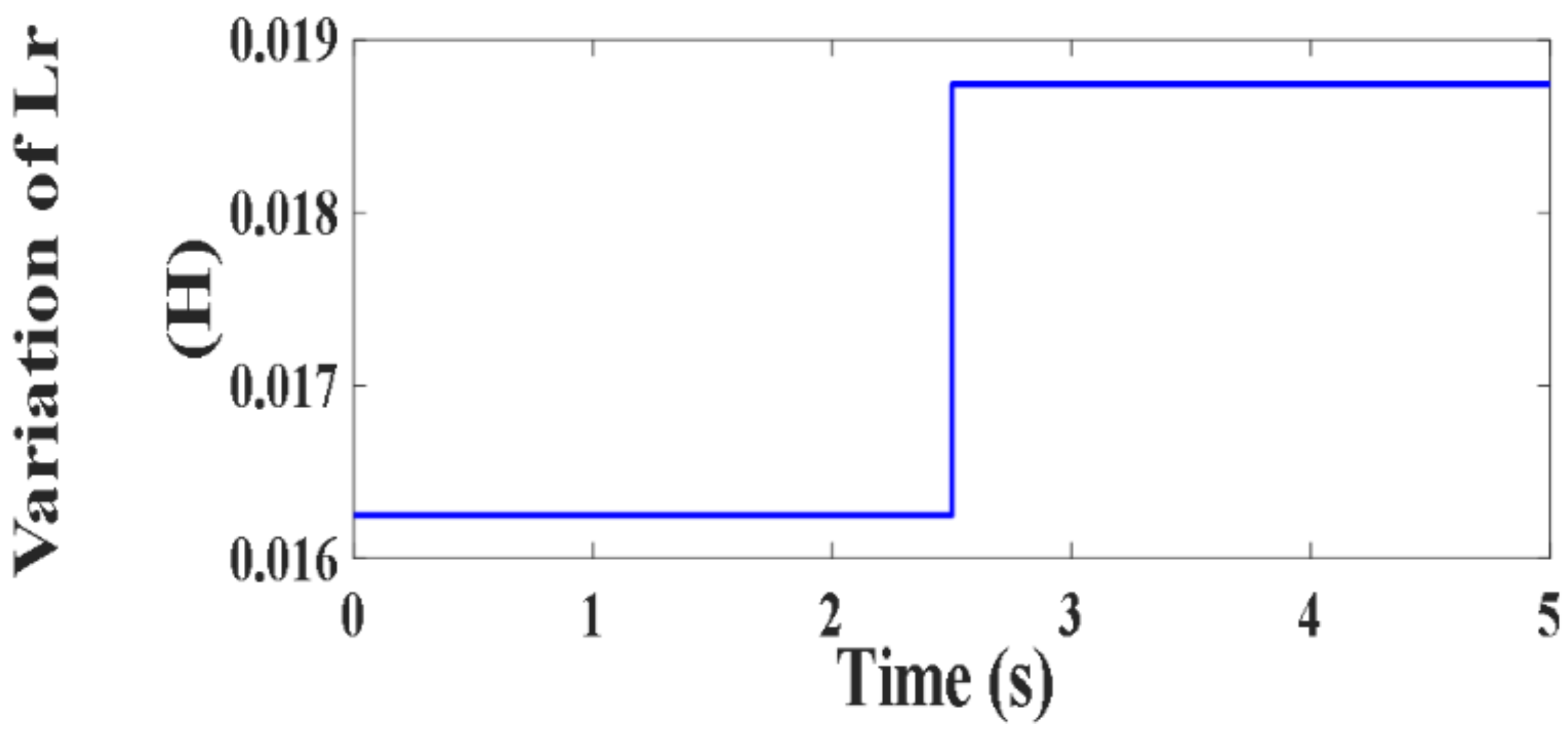
4.5.4. Testing under Proposed PVC with 15% Variation of L_r

The performance of the DFIG under PVC was also tested for the variable speed operation (Figure 101) while considering a mismatch of 15% in the stator inductance (L_r) value (Figure 102). The obtained results for the active and reactive powers, torque and rotor flux are presented in Figure 103, Figure 104, Figure 105 and Figure 106. A similar test is applied under the fixed speed operation (Figure 107) with a L_r variation (Figure 108), and the results are presented in Figure 109, Figure 110, Figure 111 and Figure 112, respectively. The captured figures confirm the ability of the designed PVC to keep the actual values within their predefined references.

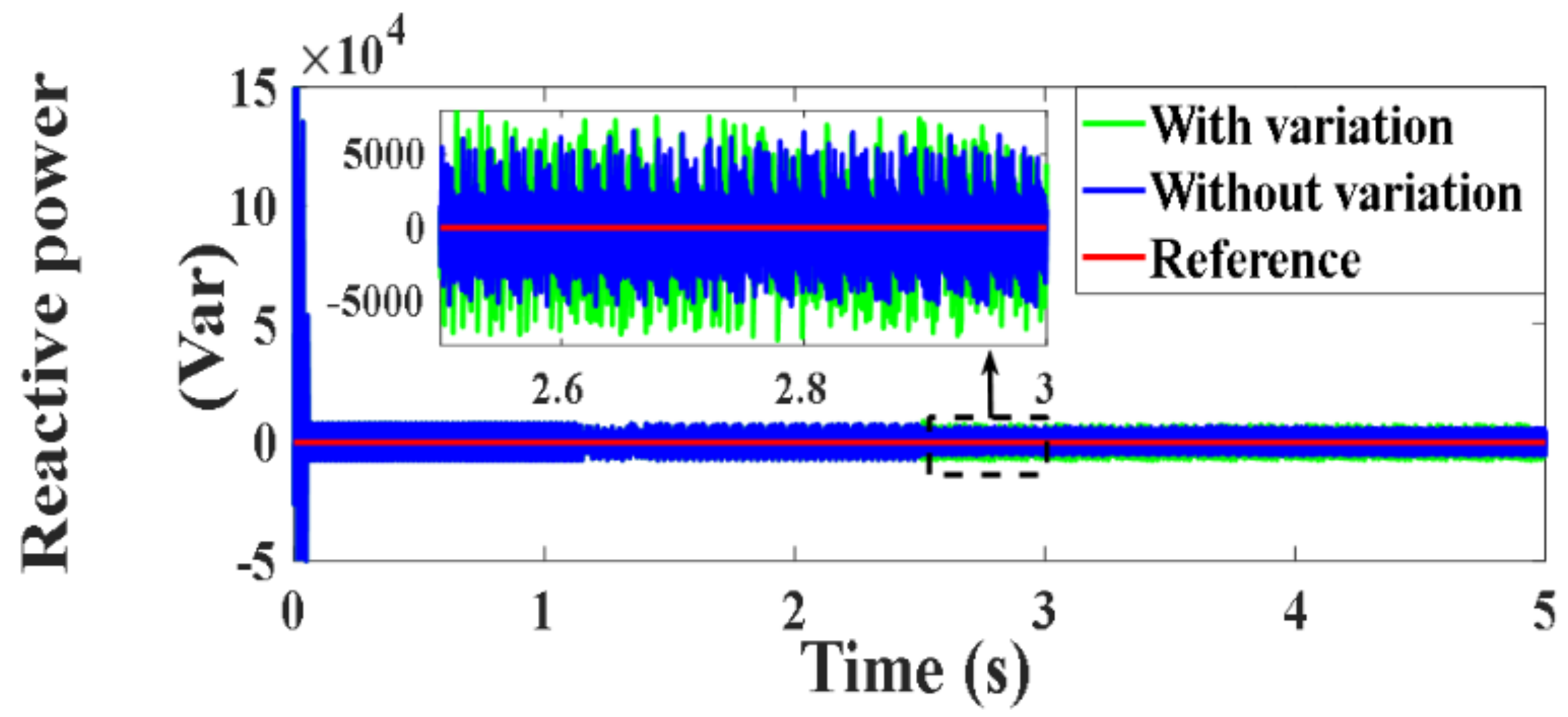
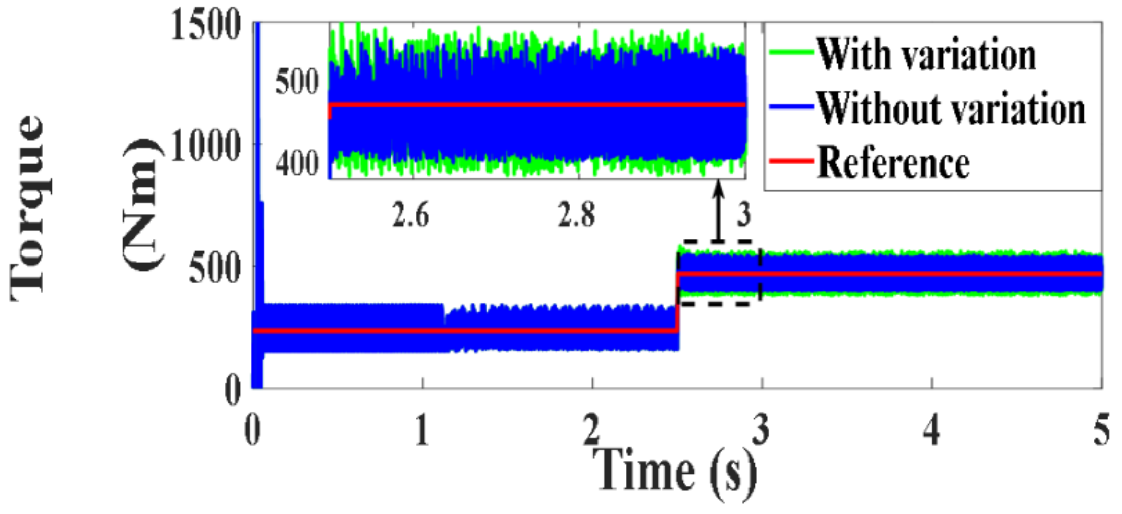
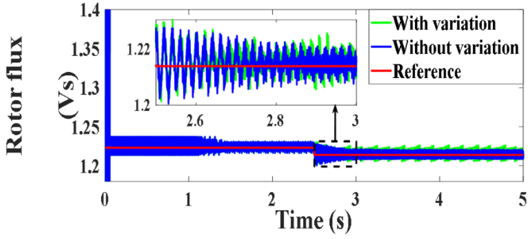
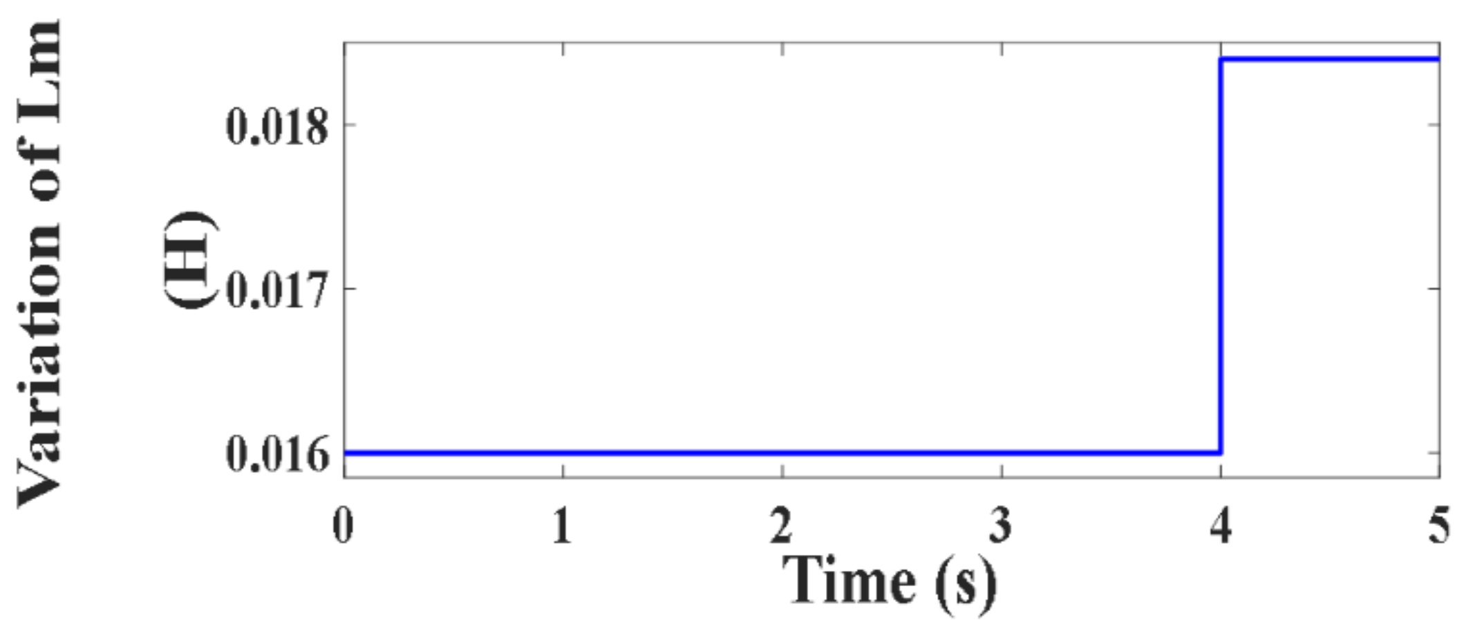
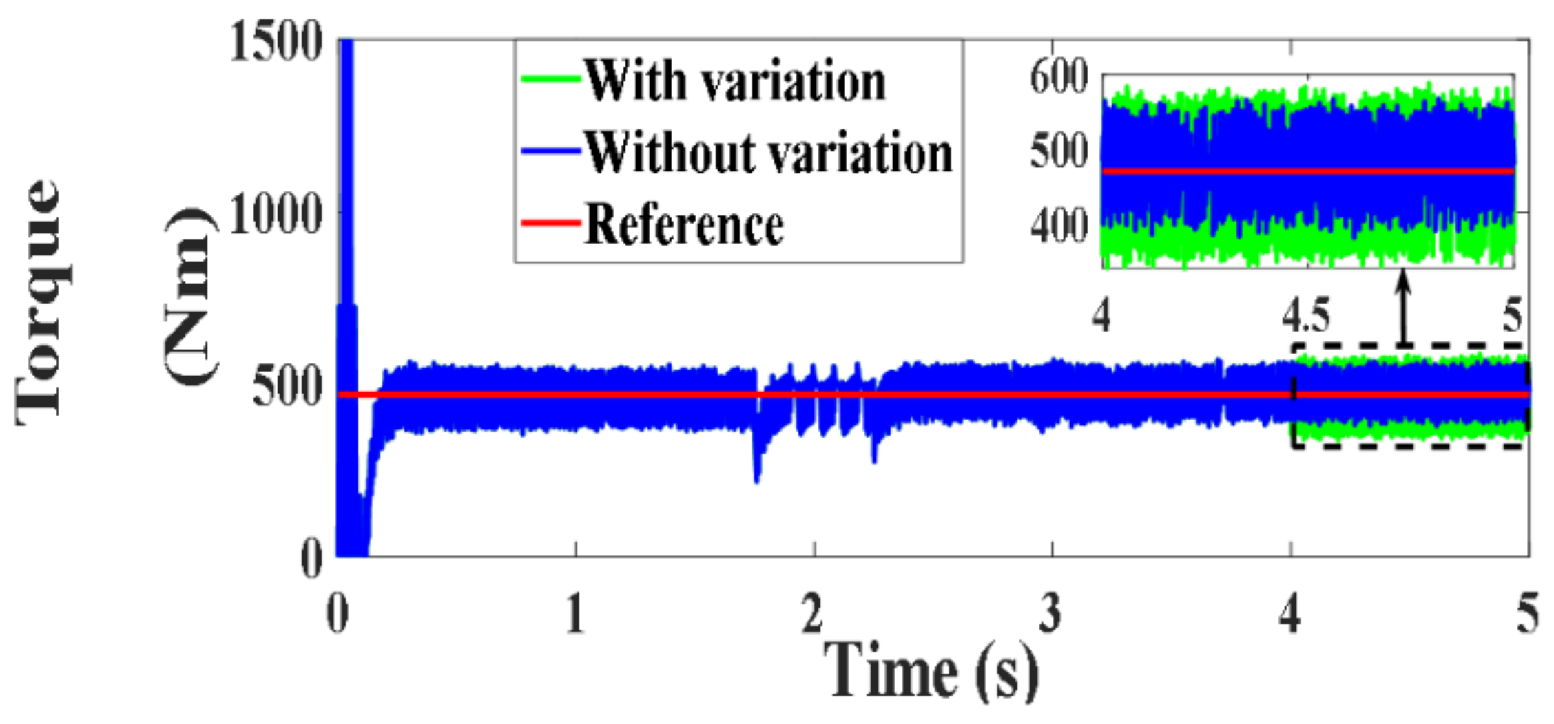
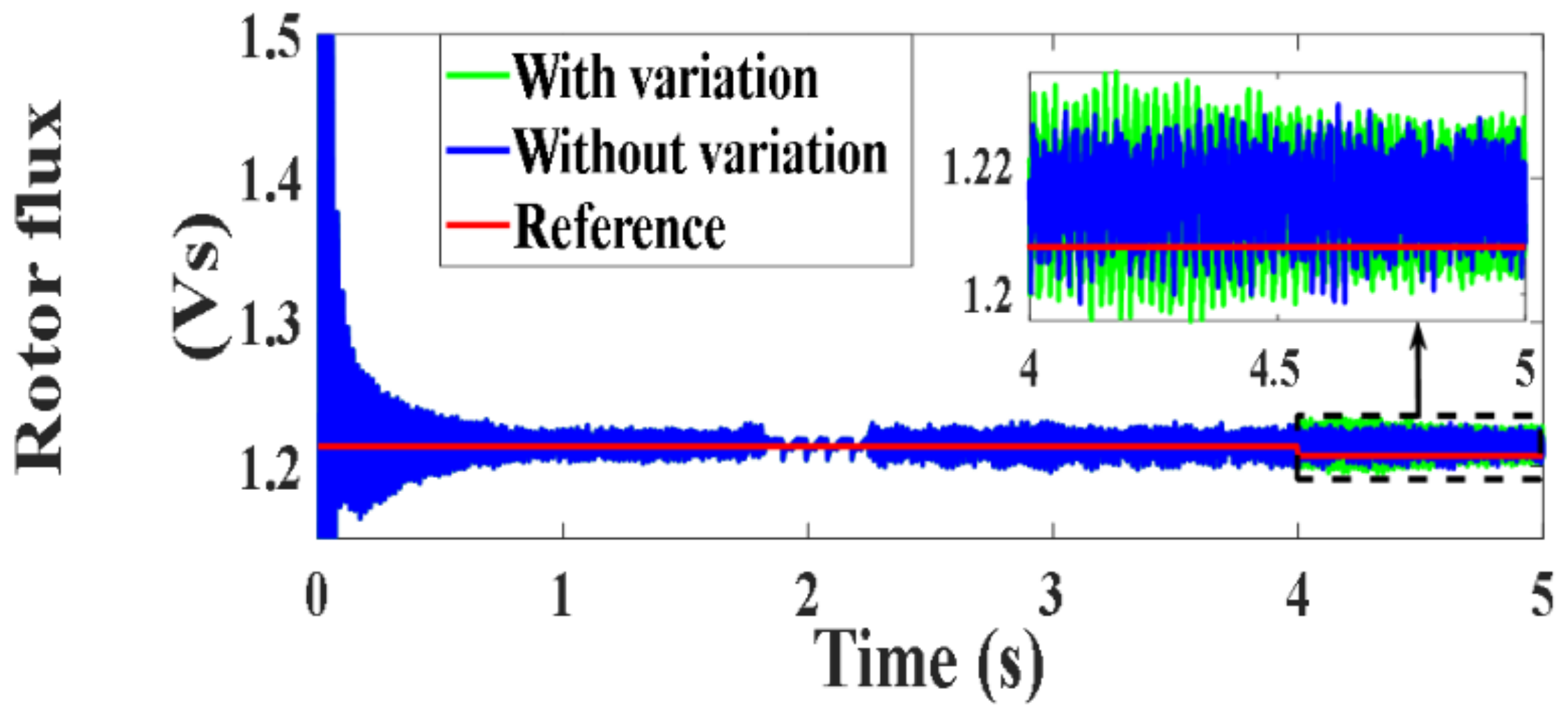
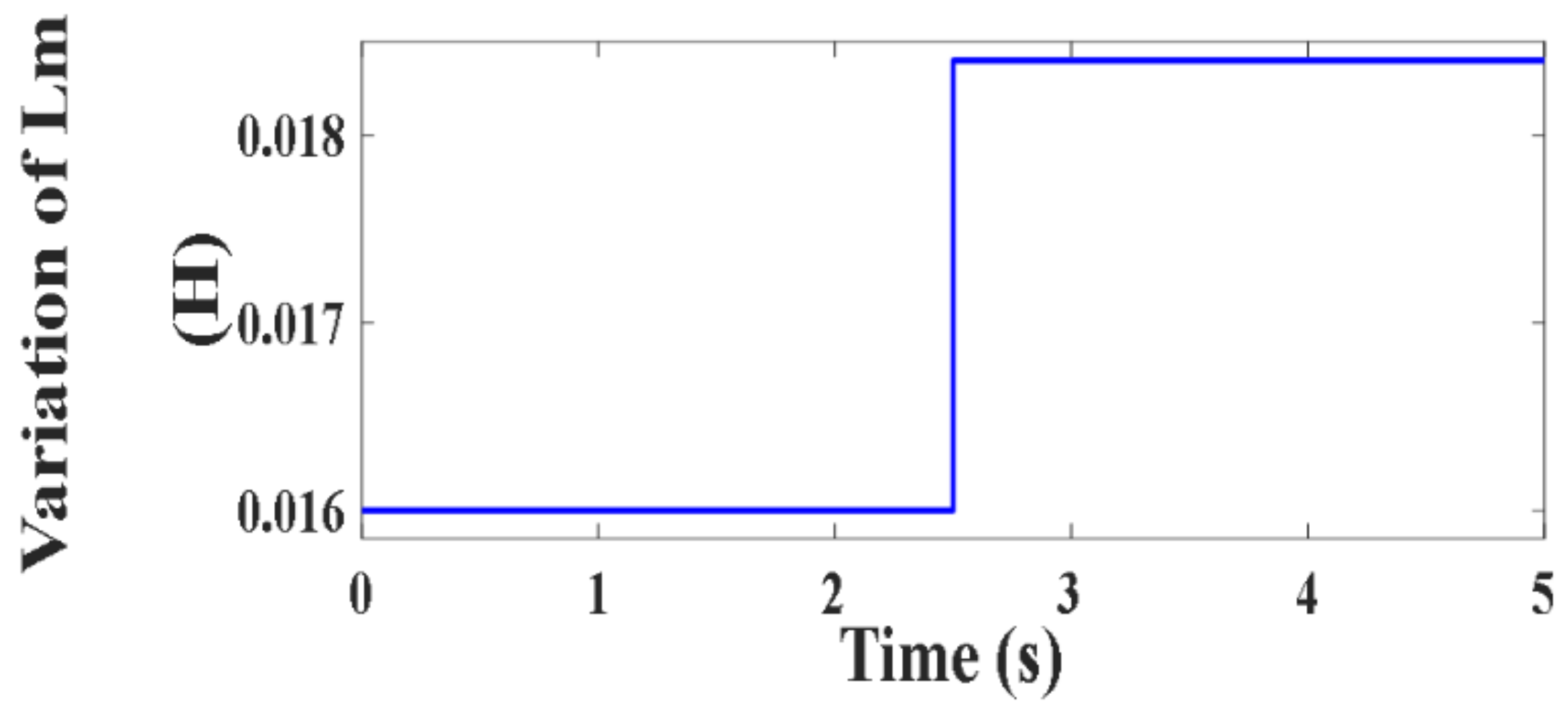
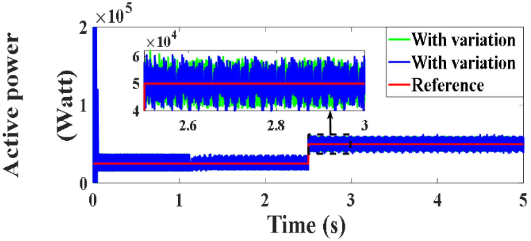
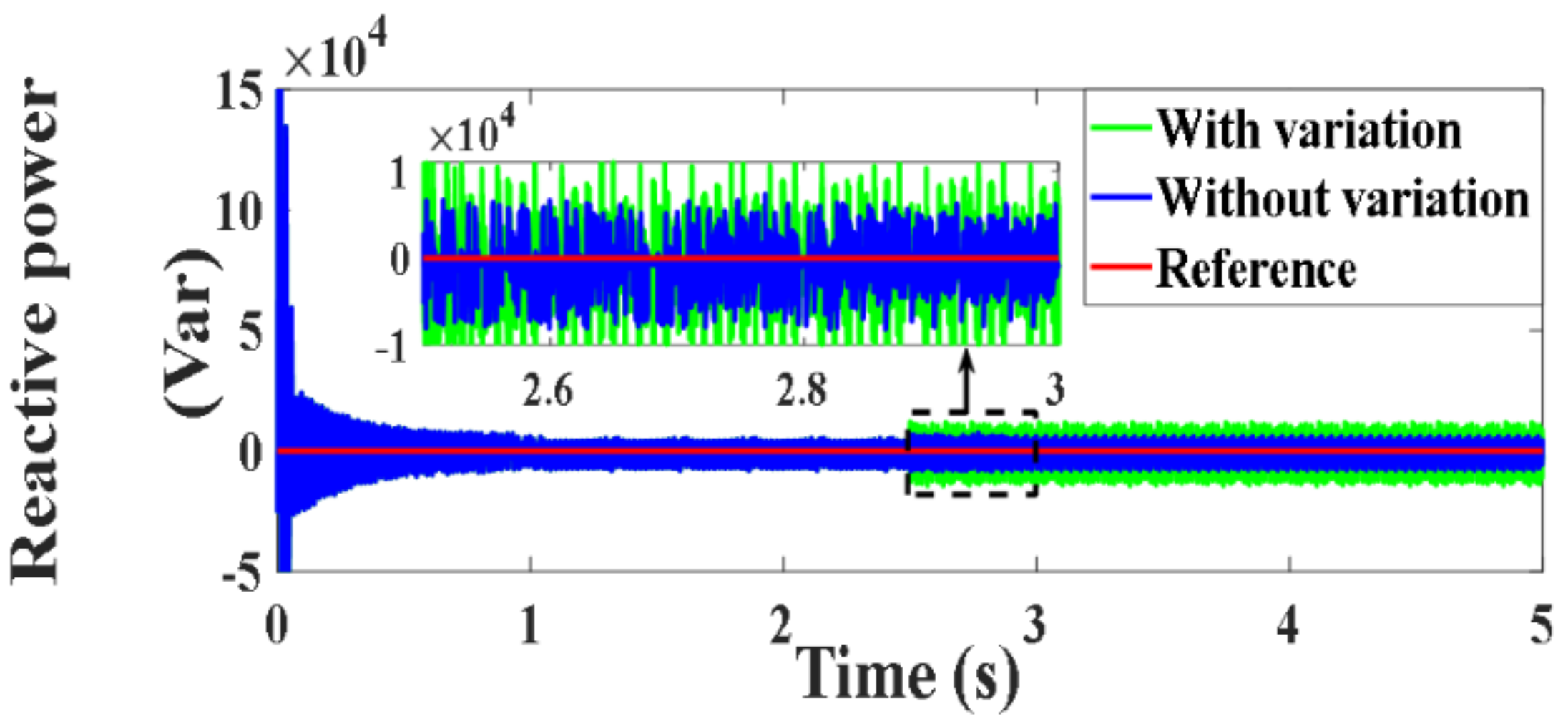
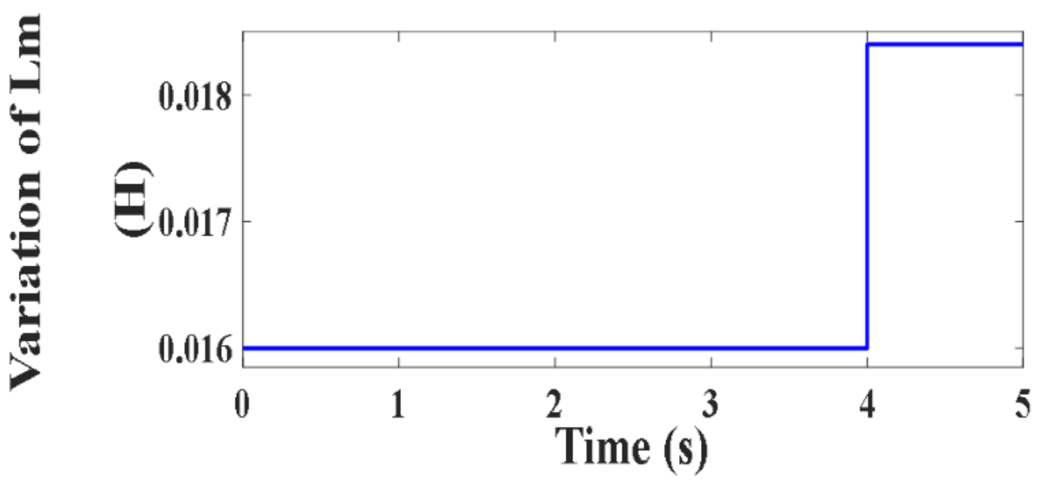
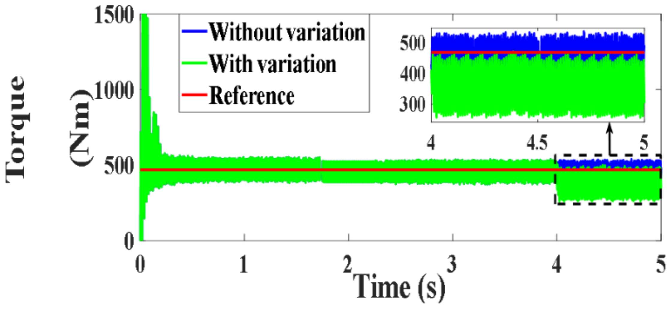
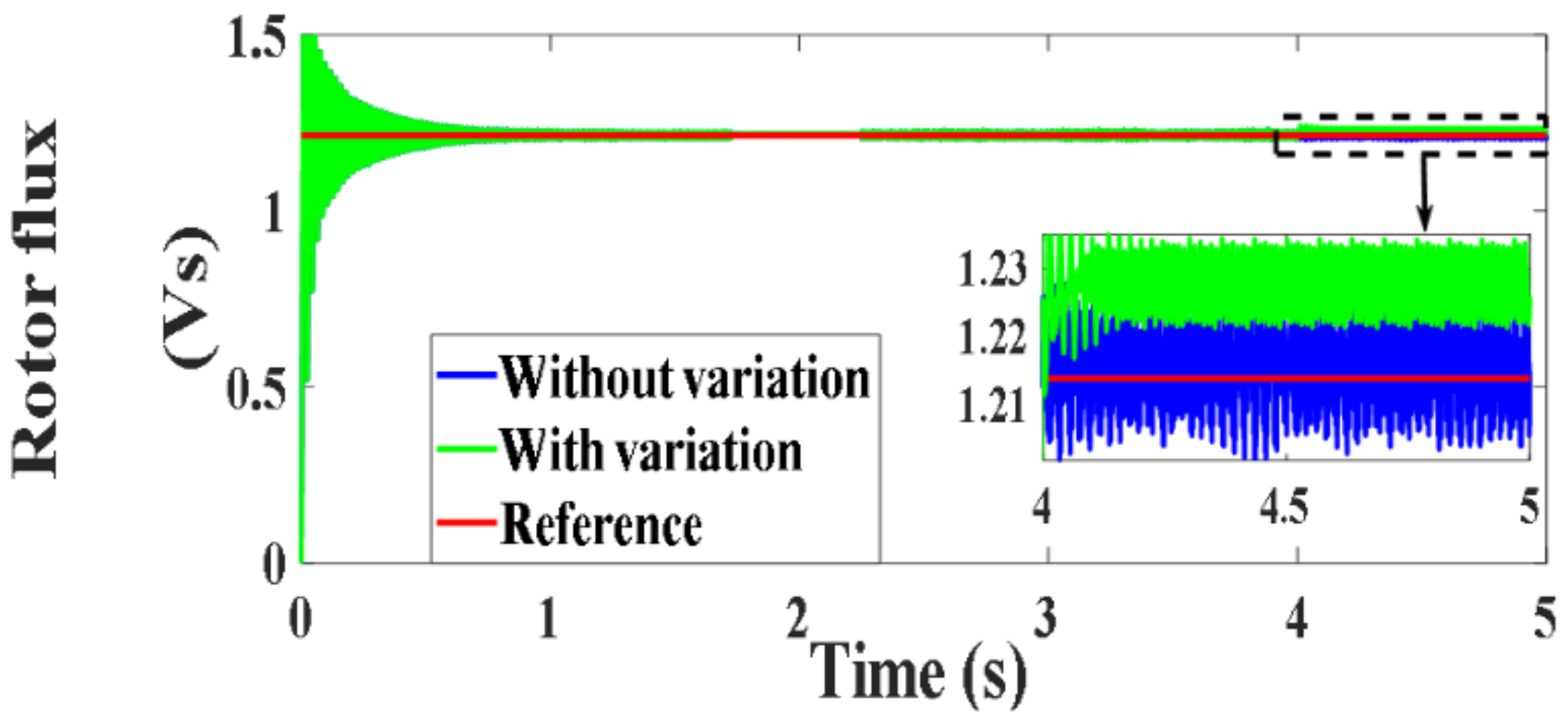
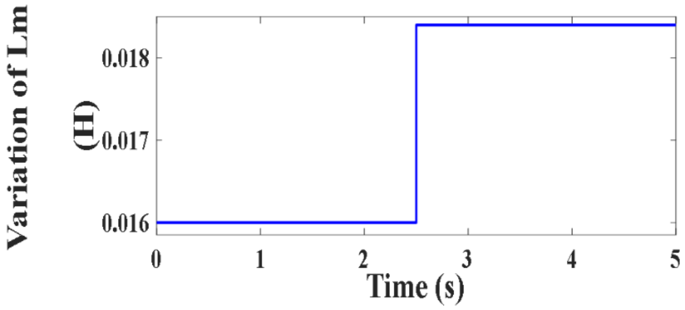
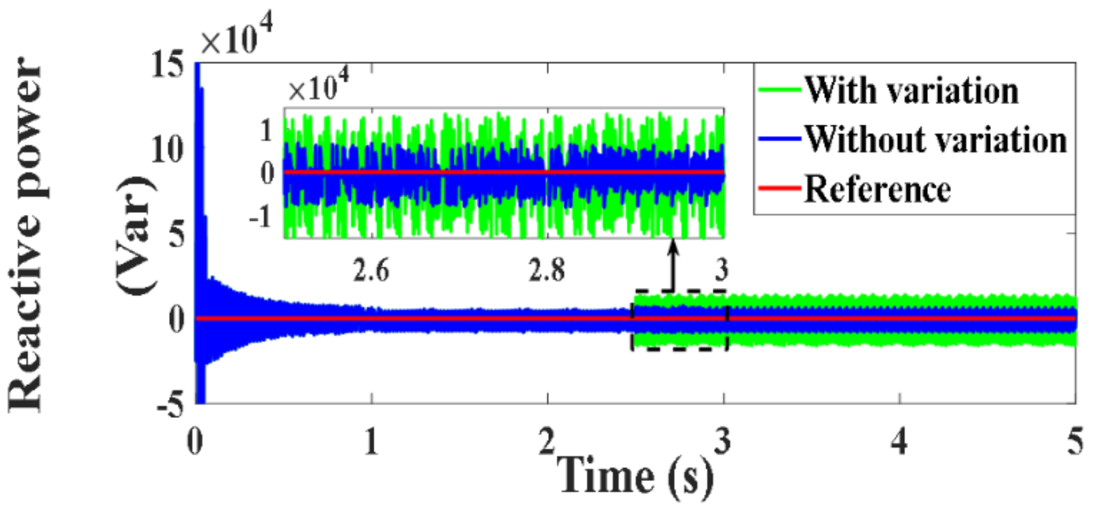
4.5.5. Testing under Proposed PVC with 15% Variation of L_m

The last performance test of the DFIG for the variable speed operation (Figure 113) while considering a mismatch of 15% in the magnetizing inductance (L_m) value (Figure 114). The obtained results for the active and reactive powers, torque and rotor flux are presented in Figure 115, Figure 116, Figure 117 and Figure 118. A similar test is applied under the fixed speed operation (Figure 119) with a L_m variation (Figure 120), and the results are presented in Figure 121, Figure 122, Figure 123 and Figure 124, respectively. The results reveal that the actual variables still stayed within their relevant reference ranges, which validates the effectiveness of the designed PVC.

4.6. Testing Using Deadbeat Based Predictive Control (DBPC) Scheme with Parameter Variation

4.6.1. Testing the DBPC Scheme with 20% Variation of R_s

In order to visualize the performance of the DFIG under the PVC technique, which uses the deadbeat principle [55,56,57,58] for generating the reference voltages under parameter mismatch, the following tests were performed. Section 4.6.1 presents the dynamic performance of the DFIG for variable speed operation (Figure 125) when a mismatch in stator resistance of 20% was applied at time t = 4 s (Figure 126). The obtained results reveal that this scheme of PVC failed in maintaining the proper operation under the resistance variation. This fact can be confirmed by following up the deviation of the actual values of active and reactive powers, torque and rotor flux (Figure 127, Figure 128, Figure 129 and Figure 130, respectively). A similar test under fixed speed operation (Figure 131) is applied with a resistance variation at time t = 2.5 s (Figure 132). The obtained results in Figure 133, Figure 134, Figure 135 and Figure 136 reveal the obvious deviation of the actual values from their references. As a result, it is confirmed that the validity and robustness of our designed PVC against parameter change compared with this scheme is ensured.

4.6.2. Testing the DBPC Scheme with 20% Variation of R_r

The dynamic performance of the DFIG for variable speed operation (Figure 137) when a mismatch in rotor resistance of 20% was applied (Figure 138). The obtained results reveal that DBPC scheme failed in maintaining the proper operation under the resistance variation. This fact can be confirmed by following up the deviation of the actual values of active and reactive powers, torque and rotor flux (Figure 139, Figure 140, Figure 141 and Figure 142, respectively). A similar test under fixed speed operation (Figure 143) is applied with a resistance variation at time t = 2.5 s (Figure 144). The obtained results in Figure 145, Figure 146, Figure 147 and Figure 148 reveal the obvious deviation of the actual values from their references.

4.6.3. Testing the DBPC Scheme with 15% Variation of L_s

The performance of the DFIG under the DBPC scheme was also tested while considering a mismatch of 15% in the stator inductance (L_s) value. For the variable speed operation (Figure 149) when a mismatch in L_s of 15% was applied (Figure 150). The obtained results reveal that DBPC scheme failed in maintaining the proper operation under the inductance variation. This fact can be confirmed by following up the deviation of the actual values of active and reactive powers, torque and rotor flux (Figure 151, Figure 152, Figure 153 and Figure 154, respectively). A similar test under fixed speed operation (Figure 155) is applied with an inductance variation at time t = 2.5 s (Figure 156). The test results in Figure 157, Figure 158, Figure 159 and Figure 160 prove the effectiveness and robustness of our designed PVC against parameter change compared with the DBPC scheme.

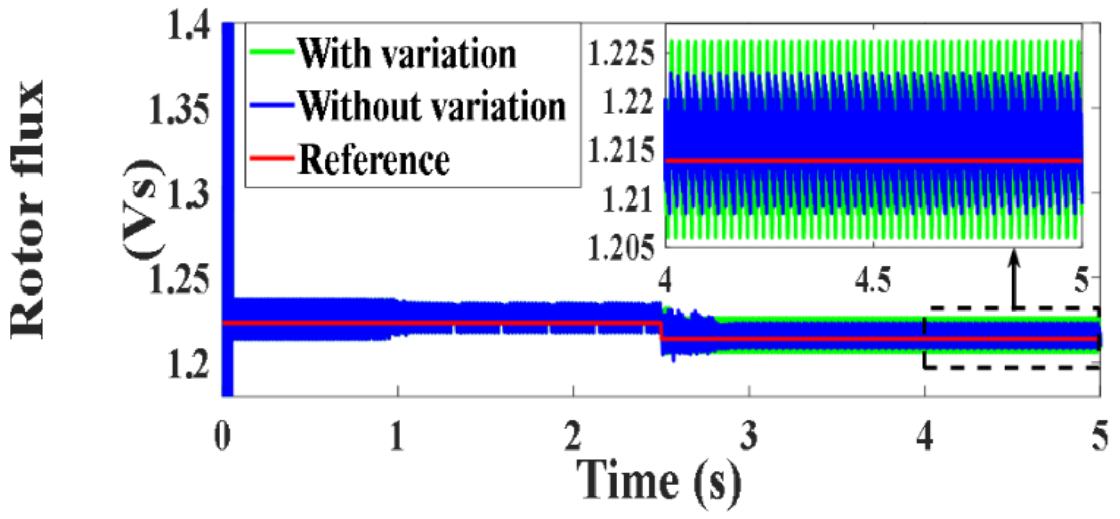
4.6.4. Testing the DBPC Scheme with 15% Variation of L_r

For the variable speed operation (Figure 161), a mismatch in L_r of 15% was applied (Figure 162). The obtained results reveal that DBPC scheme failed in maintaining the proper operation under the inductance variation. This fact is illustrated via checking the deviation of the actual values of active and reactive powers, torque and rotor flux (Figure 163, Figure 164, Figure 165 and Figure 166, respectively). A similar test under fixed speed operation (Figure 167) is applied with a L_r variation at time t = 2.5 s (Figure 168). The results in Figure 169, Figure 170, Figure 171 and Figure 172 reveal the deficiency of the DBPC in handling the system uncertainties.

4.6.5. Testing the DBPC Scheme with 15% Variation of L_m

The last performance test of the DFIG for the variable speed operation (Figure 173) while considering a mismatch of 15% in the magnetizing inductance (L_m) value (Figure 174). The obtained results for the active and reactive powers, torque and rotor flux are presented in Figure 175, Figure 176, Figure 177 and Figure 178. A similar test is applied under the fixed speed operation (Figure 179) with a L_m variation (Figure 180), and the results are presented in Figure 181, Figure 182, Figure 183 and Figure 184, respectively. The results reveal that the actual variables are still deviated from their relevant reference ranges under the mutual inductance variation, which validates the robustness and superiority of our proposed PVC.

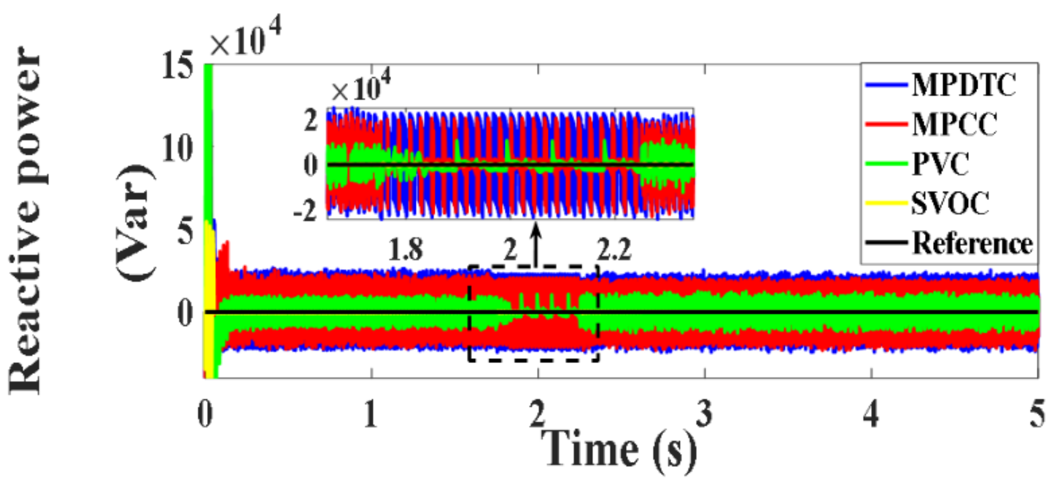
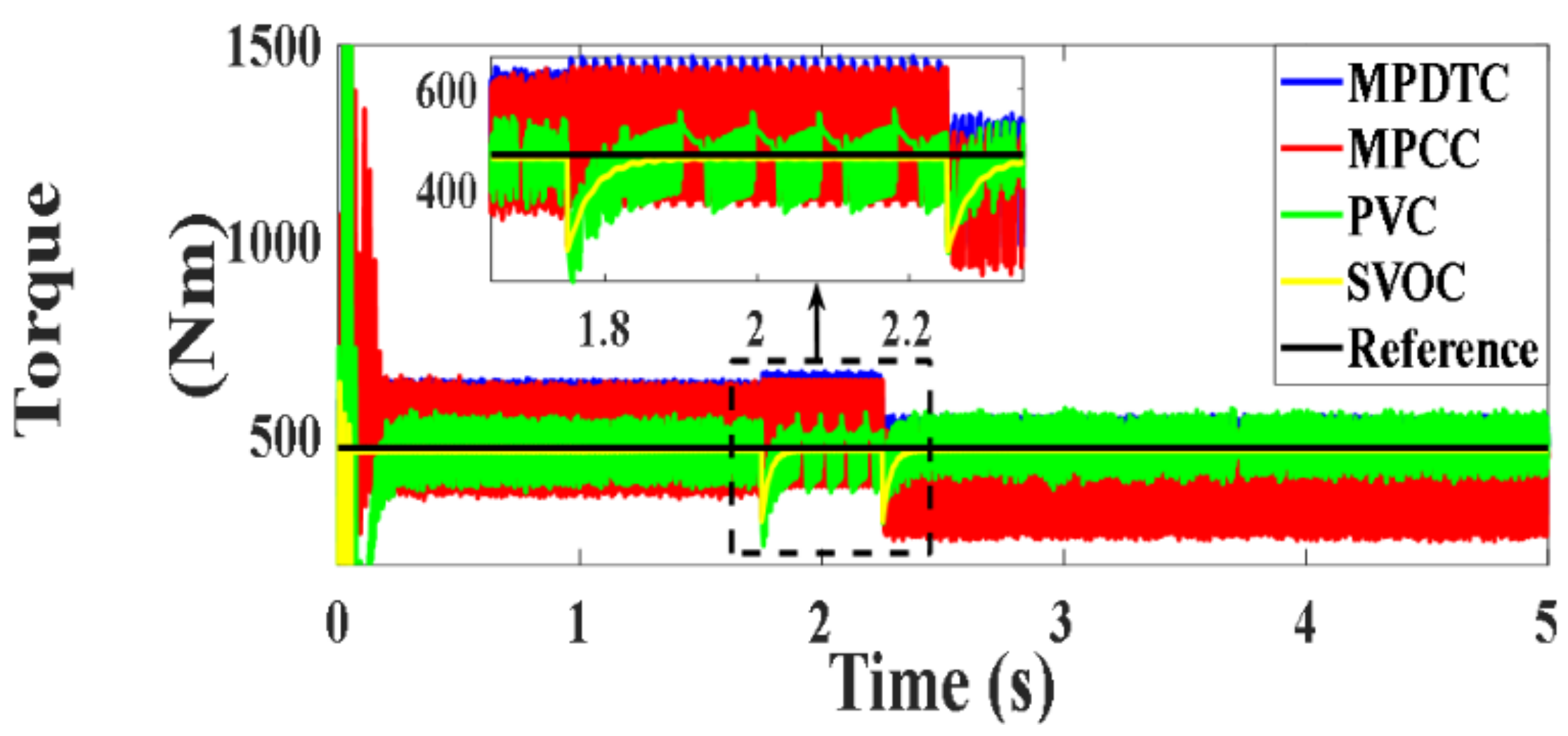
4.7. Comparison Study

Finally, a comparison was performed to study the dynamic performance of the DFIG under the four control techniques to enable the selection of the most appropriate technique to be used with the DFIG. The control effectiveness was measured in terms of ripples content, dynamic response time, and computational burden. The results are shown in Figure 185, Figure 186, Figure 187, Figure 188 and Figure 189, which outline the active power, reactive power, developed torque, and rotor flux magnitude for the variable speed operation, and illustrated in Figure 190, Figure 191, Figure 192, Figure 193 and Figure 194 the fixed speed operation, respectively.

Table 1. Response time taken by the actual values to reach to their references values in 2nd condition.

Technique	Time Taken by Active Power Profile	Time Taken by Torque Profile	Time Taken by Rotor Flux Profile
SVOC	0.55 ms	0.65 ms	6.5 ms
MPCC	0.16065 ms	0.156 ms	2.4 ms
MPDTC	0.1604 ms	0.151 ms	0.14 ms
PVC	0.14 ms	0.135 ms	0.057 ms

introduces a comparison of the response time for each technique to clarify, with the aid of the results, which technique has a shorter response time and consequently possesses the fastest dynamic response. As noted in Table 1, the actual values under the proposed PVC technique show a shorter response time in comparison with the other control approaches, as the controlled variables in PVC are the voltage vectors, which are the nearest electrical value applied to the machine windings.

Table 2. Ripples content of the actual values above their references values.

Technique	Ripples of Active Power (Watt)		Ripples of Reactive Power (var)		Ripples of Developed Torque (Nm)		Ripples of Rotor Flux (Vs)
	Case 1	Case 2	Case 1	Case 2	Case 1	Case 2	Case 1	Case 2
SVOC	740	670	274	281	9.2	9.9	0.012	0.013
MPCC	7040	7580	7865	7673	171.1	183.4	0.023	0.02
MPDTC	7890	8140	10080	9846	193.3	185	0.024	0.022
PVC	2980	3070	4043	3804	85	104.1	0.016	0.014

presents a comparison of the ripples content in the four principles and proves, with the help of the results, that the ripples content of the PVC technique is lower than that of the MPCC approach. It can thus be concluded that the proposed PVC technique is the most appropriate control scheme to be used with the DFIG for the following reasons: it achieves system simplicity; its dynamic response is the fastest compared to that of the MPCC, MPDTC, and SVOC principles; and its ripples content is lower than that of the MPCC and MPDTC approaches.

The computation time for predictive control schemes is a critical issue, as it is known that model predictive controllers are time-consuming. For this reason, a comparison was also made between the three presented predictive controllers (MPDTC, MPCC, and designed PVC) in terms of number of performed commutations during the code execution. As we know, the switching states of the inverter switches are changed as the voltage index (i) is varied, so we could identify the number of commutations using the voltage index as follows. In the beginning, for each of the three inverter legs (a, b, and c), we calculated the binary variance between each logical state and its previous one; then, we took the summation of the different resultant terms. Finally, we could easily estimate the number of performed commutations in each predictive control technique and performed a comparison between them, as illustrated in

Table 3. Comparison in terms of performed commutations by the predictive controllers.

Technique	Variable Speed Operation	Fixed Speed Operation
MPCC	8830	3732
MPDTC	8588	2461
PVC	7057	1409

. From these analytics, it was revealed that the designed PVC has the lowest number of performed commutations and thus has a shorter computation time compared with the MPDTC and MPCC approaches, which reduces the switching losses of the inverter. The used embedded code for calculating the number of performed commutations is presented in Figure 195.

5. Conclusions

The paper has presented a comprehensive dynamic performance analysis for a doubly fed induction generator using different control algorithms under different operating speeds. The control algorithms used are stator voltage-oriented control (SVOC), model predictive current control (MPCC), and model predictive direct torque control (MPDTC) as classic types and a newly formulated predictive voltage control (PVC) approach as an enhanced type. Compared with the classic predictive controllers, the cost function of the formulated PVC is very simple as it does not contain a weighting factor, in addition to not containing any variables that need to be estimated. This leads to limiting the ripples and minimizing the computation time under PVC. The finite control set (FCS) is used with the designed PVC to select the optimal voltages from a specified set of vectors, which leads to stopping the use of a PWM, thus making the system configuration simpler. The comparison results between the four controllers revealed that the proposed PVC approach succeeded in attaining the control targets and obviating the defects faced by the other control approaches. The designed PVC system improves the dynamic performance of the DFIG through presenting the fastest dynamic response, reducing the ripples content, and minimizing the number of commutations, which results in reducing the computation time. The designed PVC scheme also has a confirmed high robustness against parameter mismatch, which was illustrated through performing extensive performance evaluation tests.

References

1. Andrade, J.R.; Bessa, R.J. Improving Renewable Energy Forecasting with a Grid of Numerical Weather Predictions. IEEE Trans. Sustain. Energy 2017, 8, 1571–1580. [Google Scholar] [CrossRef] [Green Version]
2. Siano, P.; Chen, P.; Chen, Z.; Piccolo, A. Evaluating maximum wind energy exploitation in active distribution networks. Gener. Transm. Distrib. IET 2010, 4, 598–608. [Google Scholar] [CrossRef] [Green Version]
3. Tian, J.; Zhou, D.; Su, C.; Blaabjerg, F.; Chen, Z. Maximum energy yield oriented turbine control in PMSG-based wind farm. J. Eng. 2017, 2017, 2455–2460. [Google Scholar] [CrossRef]
4. Vellaipatchi, N.; Kumaresan, N.; Gounden, N. A Single Sensor Based MPPT Controller for Wind-Driven Induction Generators Supplying DC Microgrid. IEEE Trans. Power Electron. 2015, 31, 1161–1172. [Google Scholar]
5. Dambrosio, L.; Fortunato, B. One-step-ahead adaptive control of a wind-driven, synchronous generator system. Energy 1999, 24, 9–20. [Google Scholar] [CrossRef]
6. Mahmoud, M.M.; Aly, M.M.; Salama, H.S.; Abdel-Rahim, A.-M.M. Dynamic evaluation of optimization techniques–based proportional–integral controller for wind-driven permanent magnet synchronous generator. Wind Eng. 2020, 45, 696–709. [Google Scholar] [CrossRef]
7. Lopes, L.A.C.; Almeida, R.G. Wind-driven self-excited induction generator with voltage and frequency regulated by a reduced-rating voltage source inverter. IEEE Trans. Energy Convers. 2006, 21, 297–304. [Google Scholar] [CrossRef]
8. Mossa, M.A.; Gam, O.; Bianchi, N. Dynamic Performance Enhancement of a Renewable Energy System for Grid Connection and Stand-alone Operation with Battery Storage. Energies 2022, 15, 1002. [Google Scholar] [CrossRef]
9. Shaltout, A.A.; Abdel-Halim, M.A. Solid-State Control of a Wind-Driven Self-Excited Induction Generator. Electr. Mach. Power Syst. 1995, 23, 571–582. [Google Scholar] [CrossRef]
10. Puchalapalli, S.; Tiwari, S.K.; Singh, B.; Goel, P.K. A Microgrid Based on Wind-DrivenDFIG, DG, and Solar PV Array for Optimal Fuel Consumption. IEEE Trans. Ind. Appl. 2020, 56, 4689–4699. [Google Scholar] [CrossRef]
11. Mossa, M.A.; Bolognani, S. High performance Direct Power Control for a doubly fed induction generator. In Proceedings of the IECON 2016—42nd Annual Conference of the IEEE Industrial Electronics Society, Florence, Italy, 24–27 October 2016; pp. 1930–1935. [Google Scholar]
12. Marques, G.D.; Iacchetti, M.F. DFIG Topologies for DC Networks: A Review on Control and Design Features. IEEE Trans. Power Electron. 2019, 34, 1299–1316. [Google Scholar] [CrossRef]
13. Hassan, A.A.; El-Sawy, A.M.; Kamel, O.M. Direct Torque Control of a Doubly fed Induction Generator Driven by a Variable Speed Wind Turbine. JES J. Eng. Sci. 2013, 41, 199–216. [Google Scholar] [CrossRef]
14. Charles, C.M.R.; Vinod, V.; Jacob, A. Field Oriented Control of DFIG Based Wind Energy System Using Battery Energy Storage System. Procedia Technol. 2016, 24, 1203–1210. [Google Scholar] [CrossRef] [Green Version]
15. Pura, P.; Iwański, G. Rotor Current Feedback Based Direct Power Control of a Doubly Fed Induction Generator Operating with Unbalanced Grid. Energies 2021, 14, 3289. [Google Scholar] [CrossRef]
16. Mahfoud, S.; Derouich, A.; EL Ouanjli, N.; EL Mahfoud, M.; Taoussi, M. A New Strategy-Based PID Controller Optimized by Genetic Algorithm for DTC of the Doubly Fed Induction Motor. Systems 2021, 9, 37. [Google Scholar] [CrossRef]
17. Hassan, A.A.; Mohamed, Y.S.; El-Sawy, A.M.; Mossa, M.A. Control of a Wind Driven DFIG Connected to the Grid Based on Field Orientation. Wind Eng. 2011, 35, 127–143. [Google Scholar] [CrossRef]
18. Amalorpavaraj, R.A.J.; Kaliannan, P.; Padmanaban, S.; Subramaniam, U.; Ramachandaramurthy, V.K. Improved Fault Ride Through Capability in DFIG Based Wind Turbines Using Dynamic Voltage Restorer with Combined Feed-Forward and Feed-Back Control. IEEE Access 2017, 5, 20494–20503. [Google Scholar] [CrossRef]
19. Mossa, M.; Mohamed, Y. Novel Scheme for Improving the Performance of a Wind Driven Doubly Fed Induction Generator During Grid Fault. Wind Eng. 2012, 36, 305–334. [Google Scholar] [CrossRef]
20. Huang, Q.; Zou, X.; Zhu, D.; Kang, Y. Scaled Current Tracking Control for Doubly Fed Induction Generator to Ride-Through Serious Grid Faults. in IEEE Trans. Power Electron. 2016, 31, 2150–2165. [Google Scholar] [CrossRef]
21. Mossa, M.A.; Echeikh, H.; Diab, A.A.Z.; Quynh, N.V. Effective Direct Power Control for a Sensor-Less Doubly Fed Induction Generator with a Losses Minimization Criterion. Electronics 2020, 9, 1269. [Google Scholar] [CrossRef]
22. Mossa, M.A.; Al-Sumaiti, A.S.; Do, T.D.; Diab, A.A.Z. Cost-Effective Predictive Flux Control for a Sensorless Doubly Fed Induction Generator. IEEE Access 2019, 7, 172606–172627. [Google Scholar] [CrossRef]
23. Prasad, R.M.; Mulla, M.A. Mathematical Modeling and Position-Sensorless Algorithm for Stator-Side Field-Oriented Control of Rotor-Tied DFIG in Rotor Flux Reference Frame. IEEE Trans. Energy Convers. 2020, 35, 631–639. [Google Scholar] [CrossRef]
24. Amrane, F.; Chaiba, A.; Francois, B.; Babes, B. Experimental design of stand-alone field oriented control for WECS in variable speed DFIG-based on hysteresis current controller. In Proceedings of the 15th International Conference on Electrical Machines, Drives and Power Systems (ELMA), Sofia, Bulgaria, 1–3 June 2017; pp. 304–308. [Google Scholar]
25. Elmahfoud, M.; Bossoufi, B.; Taoussi, M.; Ouanjli, N.E.; Derouich, A. Rotor Field Oriented Control of Doubly Fed Induction Motor. In Proceedings of the 2019 5th International Conference on Optimization and Applications (ICOA), Kenitra, Morocco, 25–26 April 2019; pp. 1–6. [Google Scholar]
26. Arbi, J.; Ghorbal, M.J.; Slama-Belkhodja, I.; Charaabi, L. Direct Virtual Torque Control for Doubly Fed Induction Generator Grid Connection. IEEE Trans. Ind. Electron. 2009, 56, 4163–4173. [Google Scholar] [CrossRef]
27. Gundavarapu, A.; Misra, H.; Jain, A.K. Direct Torque Control Scheme for DC Voltage Regulation of the Standalone DFIG-DC System. IEEE Trans. Ind. Electron. 2017, 64, 3502–3512. [Google Scholar] [CrossRef]
28. Kashkooli, M.R.A.; Madani, S.M.; Lipo, T.A. Improved Direct Torque Control for a DFIG under Symmetrical Voltage Dip With Transient Flux Damping. IEEE Trans. Ind. Electron. 2020, 67, 28–37. [Google Scholar] [CrossRef]
29. El Daoudi, S.; Lazrak, L.; El Ouanjli, N.; Lafkih, M.A. Sensorless fuzzy direct torque control of induction motor with sliding mode speed controller. Comput. Electr. Eng. 2021, 96, 107490. [Google Scholar] [CrossRef]
30. Rodrigues, L.L.; Vilcanqui, O.A.; Murari, A.L.; Filho, A.J. Predictive Power Control for DFIG: A FARE-Based Weighting Matrices Approach. IEEE J. Emerg. Sel. Top. Power Electron. 2019, 7, 967–975. [Google Scholar] [CrossRef]
31. Mossa, M.A.; Bolognani, S. Robust Predictive Current Control for a Sensorless IM Drive Based on Torque Angle Regulation. In Proceedings of the 2019 IEEE Conference on Power Electronics and Renewable Energy (CPERE), Aswan City, Egypt, 23–25 October 2019; pp. 302–308. [Google Scholar]
32. Filho, A.J.S.; Oliveira, A.L.d.; Rodrigues, L.L.; Costa, E.C.M.; Jacomini, R.V. A Robust Finite Control Set Applied to the DFIG Power Control. IEEE J. Emerg. Sel. Top. Power Electron. 2018, 6, 1692–1698. [Google Scholar] [CrossRef]
33. Bektache, A.; Boukhezzar, B. Nonlinear predictive control of a DFIG-based wind turbine for power capture optimization. Int. J. Electr. Power Energy Syst. 2018, 101, 92–102. [Google Scholar] [CrossRef]
34. Cheng, C.; Nian, H. Low-Complexity Model Predictive Stator Current Control of DFIG Under Harmonic Grid Voltages. IEEE Trans. Energy Convers. 2017, 32, 1072–1080. [Google Scholar] [CrossRef]
35. Mossa, M.A.; Kamel, O.M.; Bolognani, S. Explicit Predictive Voltage Control for an Induction Motor Drive. In Proceedings of the 2019 21st International Middle East Power Systems Conference (MEPCON), Cairo, Egypt, 17–19 December 2019; pp. 258–264. [Google Scholar]
36. Bonfiglio, A.; Cantoni, F.; Oliveri, A.; Procopio, R.; Rosini, A.; Invernizzi, M.; Storace, M. An MPC-Based Approach for Emergency Control Ensuring Transient Stability in Power Grids With Steam Plants. IEEE Trans. Ind. Electron. 2019, 66, 5412–5422. [Google Scholar] [CrossRef]
37. Morstyn, T.; Hredzak, B.; Aguilera, R.P.; Agelidis, V.G. Model Predictive Control for Distributed Microgrid Battery Energy Storage Systems. IEEE Trans. Control Syst. Technol. 2018, 26, 1107–1114. [Google Scholar] [CrossRef] [Green Version]
38. Kou, P.; Liang, D.; Li, J.; Gao, L.; Ze, Q. Finite-Control-Set Model Predictive Control for DFIG Wind Turbines. IEEE Trans. Autom. Sci. Eng. 2018, 15, 1004–1013. [Google Scholar] [CrossRef]
39. Zanelli, A.; Kullick, J.; Eldeeb, H.M.; Frison, G.; Hackl, C.M.; Diehl, M. Continuous Control Set Nonlinear Model Predictive Control of Reluctance Synchronous Machines. IEEE Trans. Control. Syst. Technol. 2021, 30, 130–141. [Google Scholar] [CrossRef]
40. Petkar, S.; Thippiripati, V.K. Enhanced Predictive Current Control of PMSM Drive with Virtual Voltage Space Vectors. IEEE J. Emerg. Sel. Top. Ind. Electron. 2021. [Google Scholar] [CrossRef]
41. Liu, M.; Chan, K.W.; Hu, J.; Xu, W.; Rodriguez, J. Model Predictive Direct Speed Control With Torque Oscillation Reduction for PMSM Drives. IEEE Trans. Ind. Inform. 2019, 15, 4944–4956. [Google Scholar] [CrossRef]
42. Mokhtari, M.; Davari, S.A. Predictive torque control of DFIG with torque ripple reduction. In Proceedings of the 2016 IEEE International Conference on Power and Energy (PECon), Melaka, Malaysia, 28–29 November 2016; pp. 763–768. [Google Scholar]
43. Zhang, Y.; Zhu, J.; Hu, J. Model predictive direct torque control for grid synchronization of doubly fed induction generator. In Proceedings of the 2011 IEEE International Electric Machines & Drives Conference (IEMDC), Niagara Falls, ON, Canada, 15–18 May 2011; pp. 765–770. [Google Scholar]
44. Mossa, M.A.; Bolognani, S. Effective sensorless model predictive direct torque control for a doubly fed induction machine. In Proceedings of the 2017 IEEE Nineteenth International Middle East Power Systems Conference (MEPCON), Cairo, Egypt, 19–21 December 2017; pp. 1201–1207. [Google Scholar]
45. Wei, X.; Cheng, M.; Zhu, J.; Yang, H.; Luo, R. Finite-Set Model Predictive Power Control of Brushless Doubly Fed Twin Stator Induction Generator. IEEE Trans. Power Electron. 2019, 34, 2300–2311. [Google Scholar] [CrossRef]
46. Vayeghan, M.M.; Davari, S.A. Torque ripple reduction of DFIG by a new and robust predictive torque control method. IET Renew. Power Gener. 2017, 11, 1345–1352. [Google Scholar] [CrossRef]
47. Zhang, Y.; Jiao, J.; Xu, D.; Jiang, D.; Wang, Z.; Tong, C. Model Predictive Direct Power Control of Doubly Fed Induction Generators Under Balanced and Unbalanced Network Conditions. IEEE Trans. Ind. Appl. 2020, 56, 771–786. [Google Scholar] [CrossRef]
48. Zarei, M.E.; Nicolás, C.V.; Arribas, J.R. Improved Predictive Direct Power Control of Doubly Fed Induction Generator During Unbalanced Grid Voltage Based on Four Vectors. IEEE J. Emerg. Sel. Top. Power Electron. 2017, 5, 695–707. [Google Scholar] [CrossRef]
49. Davari, S.A.; Nekoukar, V.; Garcia, C.; Rodriguez, J. Online Weighting Factor Optimization by Simplified Simulated Annealing for Finite Set Predictive Control. IEEE Trans. Ind. Inform. 2021, 17, 31–40. [Google Scholar] [CrossRef]
50. Mossa, M.A.; Bolognani, S. Effective model predictive current control for a sensorless IM drive. In Proceedings of the 2017 IEEE International Symposium on Sensorless Control for Electrical Drives (SLED), Catania, Italy, 18–19 September 2017; pp. 37–42. [Google Scholar]
51. Bozorgi, A.M.; Farasat, M.; Jafarishiadeh, S. Model predictive current control of surface-mounted permanent magnet synchronous motor with low torque and current ripple. IET Power Electron. 2017, 10, 1120–1128. [Google Scholar] [CrossRef]
52. Mossa, M.A.; Bolognani, S. Predictive Power Control for a Linearized Doubly Fed Induction Generator Model. In Proceedings of the 2019 21st International Middle East Power Systems Conference (MEPCON), Cairo, Egypt, 17–19 December 2019; pp. 250–257. [Google Scholar]
53. Mossa, M.A.; Bolognani, S. A novel sensorless direct torque control for a doubly fed induction machine. In Proceedings of the 2016 XXII International Conference on Electrical Machines (ICEM), Lausanne, Switzerland, 4–7 September 2016; pp. 942–948. [Google Scholar]
54. Mossa, M.A. Field Orientation Control of a Wind Driven DFIG Connected to the Grid. Wseas Trans. Power Syst. 2012, 4, 182–197. [Google Scholar]
55. Zhang, Y.; Xu, D. Direct power control of doubly fed induction generator based on extended power theory under unbalanced grid condition. In Proceedings of the 2017 IEEE 3rd International Future Energy Electronics Conference and ECCE Asia (IFEEC 2017—ECCE Asia), Kaohsiung, Taiwan, 4–7 June 2017; pp. 992–996. [Google Scholar]
56. Osorio, C.M.R.; Chaves, J.S.S.; Murari, A.L.L.F.; Filho, A.J.S. Comparative Analysis of the Doubly Fed Induction Generator (DFIG) Under Balanced Voltage Sag Using a Deadbeat Controller. IEEE Lat. Am. Trans. 2017, 15, 869–876. [Google Scholar] [CrossRef]
57. Franco, R.; Capovilla, C.E.; Jacomini, R.V.; Altana, J.A.T.; Filho, A.J.S. A deadbeat direct power control applied to doubly-fed induction aerogenerator under normal and sag voltages conditions. In Proceedings of the IECON 2014—40th Annual Conference of the IEEE Industrial Electronics Society, Dallas, TX, USA, 29 October–1 November 2014; pp. 1906–1911. [Google Scholar]
58. Mossa, M.A.; Do, T.D.; Al-Sumaiti, A.S.; Quynh, N.V.; Diab, A.A.Z. Effective Model Predictive Voltage Control for a Sensorless Doubly Fed Induction Generator. IEEE Can. J. Electr. Comput. Eng. 2021, 44, 50–64. [Google Scholar] [CrossRef]
Figure 1. FCS PC structure.
Processes 10 00456 g001
Figure 2. CCS PC structure.
Processes 10 00456 g002
Figure 3. Equivalent circuit model of DFIG.
Processes 10 00456 g003
Figure 4. Relationships between reference frames.
Processes 10 00456 g004
Figure 5. SVOC technique for the DFIG.
Processes 10 00456 g005
Figure 6. MPCC technique for the DFIG.
Processes 10 00456 g006
Figure 7. MPDTC technique for the DFIG.
Processes 10 00456 g007
Figure 8. Proposed PVC technique for the DFIG.
Processes 10 00456 g008
Figure 9. Prime mover operating speeds (rad/s).
Processes 10 00456 g009
Figure 10. Active power under SVOC (Watt).
Processes 10 00456 g010
Figure 11. Reactive power under SVOC (var).
Processes 10 00456 g011
Figure 12. Developed torque under SVOC (Nm).
Processes 10 00456 g012
Figure 13. Rotor flux under SVOC (Vs).
Processes 10 00456 g013
Figure 14. Stator currents under SVOC (A).
Processes 10 00456 g014
Figure 15. Rotor currents under SVOC (A).
Processes 10 00456 g015
Figure 16. Prime mover operating speed (rad/s).
Processes 10 00456 g016
Figure 17. Active power under SVOC (Watt).
Processes 10 00456 g017
Figure 18. Reactive power under SVOC (var).
Processes 10 00456 g018
Figure 19. Developed torque under SVOC (Nm).
Processes 10 00456 g019
Figure 20. Rotor flux under SVOC (Vs).
Processes 10 00456 g020
Figure 21. Stator currents under SVOC (A).
Processes 10 00456 g021
Figure 22. Rotor currents under SVOC (A).
Processes 10 00456 g022
Figure 23. Prime mover operating speeds (rad/s).
Processes 10 00456 g023
Figure 24. Active power under MPCC (Watt).
Processes 10 00456 g024
Figure 25. Reactive power under MPCC (var).
Processes 10 00456 g025
Figure 26. Developed torque under MPCC (Nm).
Processes 10 00456 g026
Figure 27. Rotor flux under MPCC (Vs).
Processes 10 00456 g027
Figure 28. Stator currents under MPCC (A).
Processes 10 00456 g028
Figure 29. Rotor currents under MPCC (A).
Processes 10 00456 g029
Figure 30. Prime mover operating speed (rad/s).
Processes 10 00456 g030
Figure 31. Active power under MPCC (Watt).
Processes 10 00456 g031
Figure 32. Reactive power under MPCC (var).
Processes 10 00456 g032
Figure 33. Developed torque under MPCC (Nm).
Processes 10 00456 g033
Figure 34. Rotor flux under MPCC (Vs).
Processes 10 00456 g034
Figure 35. Stator currents under MPCC (A).
Processes 10 00456 g035
Figure 36. Rotor currents under MPCC (A).
Processes 10 00456 g036
Figure 37. Prime mover operating speeds (rad/s).
Processes 10 00456 g037
Figure 38. Active power under MPDTC (Watt).
Processes 10 00456 g038
Figure 39. Reactive power under MPDTC (var).
Processes 10 00456 g039
Figure 40. Torque under MPDTC (Nm).
Processes 10 00456 g040
Figure 41. Rotor flux under MPDTC (Vs).
Processes 10 00456 g041
Figure 42. Stator currents under MPDTC (A).
Processes 10 00456 g042
Figure 43. Rotor currents under MPDTC (A).
Processes 10 00456 g043
Figure 44. Prime mover operating speed (rad/s).
Processes 10 00456 g044
Figure 45. Active power under MPDTC (Watt).
Processes 10 00456 g045
Figure 46. Reactive power under MPDTC (var).
Processes 10 00456 g046
Figure 47. Torque under MPDTC (Nm).
Processes 10 00456 g047
Figure 48. Rotor flux under MPDTC (Vs).
Processes 10 00456 g048
Figure 49. Stator currents under MPDTC (A).
Processes 10 00456 g049
Figure 50. Rotor currents under MPDTC (A).
Processes 10 00456 g050
Figure 51. Prime mover operating speeds (rad/s).
Processes 10 00456 g051
Figure 52. Active power under PVC (Watt).
Processes 10 00456 g052
Figure 53. Reactive power under PVC (var).
Processes 10 00456 g053
Figure 54. Developed torque under PVC (Nm).
Processes 10 00456 g054
Figure 55. Rotor flux under PVC (Vs).
Processes 10 00456 g055
Figure 56. Stator currents under PVC (A).
Processes 10 00456 g056
Figure 57. Rotor currents under PVC (A).
Processes 10 00456 g057
Figure 58. Prime mover operating speed (rad/s).
Processes 10 00456 g058
Figure 59. Active power under PVC (Watt).
Processes 10 00456 g059
Figure 60. Reactive power under PVC (var).
Processes 10 00456 g060
Figure 61. Developed torque under PVC (Nm).
Processes 10 00456 g061
Figure 62. Rotor flux under PVC (Vs).
Processes 10 00456 g062
Figure 63. Stator currents under PVC (A).
Processes 10 00456 g063
Figure 64. Rotor currents under PVC (A).
Processes 10 00456 g064
Figure 65. Prime mover operating speeds (rad/s).
Processes 10 00456 g065
Figure 66. Variation of Rs (Ω).
Processes 10 00456 g066
Figure 67. Active power under PVC (Watt).
Processes 10 00456 g067
Figure 68. Reactive power under PVC (var).
Processes 10 00456 g068
Figure 69. Developed torque under PVC (Nm).
Processes 10 00456 g069
Figure 70. Rotor flux under PVC (Vs).
Processes 10 00456 g070
Figure 71. Prime mover operating speeds (rad/s).
Processes 10 00456 g071
Figure 72. Variation of Rs (Ω).
Processes 10 00456 g072
Figure 73. Active power under PVC (Watt).
Processes 10 00456 g073
Figure 74. Reactive power under PVC (var).
Processes 10 00456 g074
Figure 75. Developed torque under PVC (Nm).
Processes 10 00456 g075
Figure 76. Rotor flux under PVC (Vs).
Processes 10 00456 g076
Figure 77. Prime mover operating speeds (rad/s).
Processes 10 00456 g077
Figure 78. Variation of Rr (Ω).
Processes 10 00456 g078
Figure 79. Active power under PVC (Watt).
Processes 10 00456 g079
Figure 80. Reactive power under PVC (var).
Processes 10 00456 g080
Figure 81. Developed torque under PVC (Nm).
Processes 10 00456 g081
Figure 82. Rotor flux under PVC (Vs).
Processes 10 00456 g082
Figure 83. Prime mover operating speeds (rad/s).
Processes 10 00456 g083
Figure 84. Variation of Rr (Ω).
Processes 10 00456 g084
Figure 85. Active power under PVC (Watt).
Processes 10 00456 g085
Figure 86. Reactive power under PVC (var).
Processes 10 00456 g086
Figure 87. Developed torque under PVC (Nm).
Processes 10 00456 g087
Figure 88. Rotor flux under PVC (Vs).
Processes 10 00456 g088
Figure 89. Prime mover operating speeds (rad/s).
Processes 10 00456 g089
Figure 90. Variation of Ls (H).
Processes 10 00456 g090
Figure 91. Active power under PVC (Watt).
Processes 10 00456 g091
Figure 92. Reactive power under PVC (var).
Processes 10 00456 g092
Figure 93. Developed torque under PVC (Nm).
Processes 10 00456 g093
Figure 94. Rotor flux under PVC (Vs).
Processes 10 00456 g094
Figure 95. Prime mover operating speeds (rad/s).
Processes 10 00456 g095
Figure 96. Variation of Ls (H).
Processes 10 00456 g096
Figure 97. Active power under PVC (Watt).
Processes 10 00456 g097
Figure 98. Reactive power under PVC (var).
Processes 10 00456 g098
Figure 99. Developed torque under PVC (Nm).
Processes 10 00456 g099
Figure 100. Rotor flux under PVC (Vs).
Processes 10 00456 g100
Figure 101. Prime mover operating speeds (rad/s).
Processes 10 00456 g101
Figure 102. Variation of Lr (H).
Processes 10 00456 g102
Figure 103. Active power under PVC (Watt).
Processes 10 00456 g103
Figure 104. Reactive power under PVC (var).
Processes 10 00456 g104
Figure 105. Developed torque under PVC (Nm).
Processes 10 00456 g105
Figure 106. Rotor flux under PVC (Vs).
Processes 10 00456 g106
Figure 107. Prime mover operating speeds (rad/s).
Processes 10 00456 g107
Figure 108. Variation of Lr (H).
Processes 10 00456 g108
Figure 109. Active power under PVC (Watt).
Processes 10 00456 g109
Figure 110. Reactive power under PVC (var).
Processes 10 00456 g110
Figure 111. Developed torque under PVC (Nm).
Processes 10 00456 g111
Figure 112. Rotor flux under PVC (Vs).
Processes 10 00456 g112
Figure 113. Prime mover operating speeds (rad/s).
Processes 10 00456 g113
Figure 114. Variation of Lm (H).
Processes 10 00456 g114
Figure 115. Active power under PVC (Watt).
Processes 10 00456 g115
Figure 116. Reactive power under PVC (var).
Processes 10 00456 g116
Figure 117. Developed torque under PVC (Nm).
Processes 10 00456 g117
Figure 118. Rotor flux under PVC (Vs).
Processes 10 00456 g118
Figure 119. Prime mover operating speeds (rad/s).
Processes 10 00456 g119
Figure 120. Variation of Lm (H).
Processes 10 00456 g120
Figure 121. Active power under PVC (Watt).
Processes 10 00456 g121
Figure 122. Reactive power under PVC (var).
Processes 10 00456 g122
Figure 123. Developed torque under PVC (Nm).
Processes 10 00456 g123
Figure 124. Rotor flux under PVC (Vs).
Processes 10 00456 g124
Figure 125. Prime mover operating speeds (rad/s).
Processes 10 00456 g125
Figure 126. Variation of Rs (Ω).
Processes 10 00456 g126
Figure 127. Active power under PVC (Watt).
Processes 10 00456 g127
Figure 128. Reactive power under PVC (var).
Processes 10 00456 g128
Figure 129. Developed torque under PVC (Nm).
Processes 10 00456 g129
Figure 130. Rotor flux under PVC (Vs).
Processes 10 00456 g130
Figure 131. Prime mover operating speeds (rad/s).
Processes 10 00456 g131
Figure 132. Variation of Rs (Ω).
Processes 10 00456 g132
Figure 133. Active power under PVC (Watt).
Processes 10 00456 g133
Figure 134. Reactive power under PVC (var).
Processes 10 00456 g134
Figure 135. Developed torque under PVC (Nm).
Processes 10 00456 g135
Figure 136. Rotor flux under PVC (Vs).
Processes 10 00456 g136
Figure 137. Prime mover operating speeds (rad/s).
Processes 10 00456 g137
Figure 138. Variation of Rr (Ω).
Processes 10 00456 g138
Figure 139. Active power under PVC (Watt).
Processes 10 00456 g139
Figure 140. Reactive power under PVC (var).
Processes 10 00456 g140
Figure 141. Developed torque under PVC (Nm).
Processes 10 00456 g141
Figure 142. Rotor flux under PVC (Vs).
Processes 10 00456 g142
Figure 143. Prime mover operating speeds (rad/s).
Processes 10 00456 g143
Figure 144. Variation of Rr (Ω).
Processes 10 00456 g144
Figure 145. Active power under PVC (Watt).
Processes 10 00456 g145
Figure 146. Reactive power under PVC (var).
Processes 10 00456 g146
Figure 147. Developed torque under PVC (Nm).
Processes 10 00456 g147
Figure 148. Rotor flux under PVC (Vs).
Processes 10 00456 g148
Figure 149. Prime mover operating speeds (rad/s).
Processes 10 00456 g149
Figure 150. Variation of Ls (H).
Processes 10 00456 g150
Figure 151. Active power under PVC (Watt).
Processes 10 00456 g151
Figure 152. Reactive power under PVC (var).
Processes 10 00456 g152
Figure 153. Developed torque under PVC (Nm).
Processes 10 00456 g153
Figure 154. Rotor flux under PVC (Vs).
Processes 10 00456 g154
Figure 155. Prime mover operating speeds (rad/s).
Processes 10 00456 g155
Figure 156. Variation of Ls (H).
Processes 10 00456 g156
Figure 157. Active power under PVC (Watt).
Processes 10 00456 g157
Figure 158. Reactive power under PVC (var).
Processes 10 00456 g158
Figure 159. Developed torque under PVC (Nm).
Processes 10 00456 g159
Figure 160. Rotor flux under PVC (Vs).
Processes 10 00456 g160
Figure 161. Prime mover operating speeds (rad/s).
Processes 10 00456 g161
Figure 162. Variation of Lr (H).
Processes 10 00456 g162
Figure 163. Active power under PVC (Watt).
Processes 10 00456 g163
Figure 164. Reactive power under PVC (var).
Processes 10 00456 g164
Figure 165. Developed torque under PVC (Nm).
Processes 10 00456 g165
Figure 166. Rotor flux under PVC (Vs).
Processes 10 00456 g166
Figure 167. Prime mover operating speeds (rad/s).
Processes 10 00456 g167
Figure 168. Variation of Lr (H).
Processes 10 00456 g168
Figure 169. Active power under PVC (Watt).
Processes 10 00456 g169
Figure 170. Reactive power under PVC (var).
Processes 10 00456 g170
Figure 171. Developed torque under PVC (Nm).
Processes 10 00456 g171
Figure 172. Rotor flux under PVC (Vs).
Processes 10 00456 g172
Figure 173. Prime mover operating speeds (rad/s).
Processes 10 00456 g173
Figure 174. Variation of Lm (H).
Processes 10 00456 g174
Figure 175. Active power under PVC (Watt).
Processes 10 00456 g175
Figure 176. Reactive power under PVC (var).
Processes 10 00456 g176
Figure 177. Developed torque under PVC (Nm).
Processes 10 00456 g177
Figure 178. Rotor flux under PVC (Vs).
Processes 10 00456 g178
Figure 179. Prime mover operating speeds (rad/s).
Processes 10 00456 g179
Figure 180. Variation of Lm (H).
Processes 10 00456 g180
Figure 181. Active power under PVC (Watt).
Processes 10 00456 g181
Figure 182. Reactive power under PVC (var).
Processes 10 00456 g182
Figure 183. Developed torque under PVC (Nm).
Processes 10 00456 g183
Figure 184. Rotor flux under PVC (Vs).
Processes 10 00456 g184
Figure 185. Prime mover operating speeds (rad/s).
Processes 10 00456 g185
Figure 186. Comparison between active powers of four techniques (Watt).
Processes 10 00456 g186
Figure 187. Comparison between reactive powers of four techniques (var).
Processes 10 00456 g187
Figure 188. Comparison between torques of four techniques (Nm).
Processes 10 00456 g188
Figure 189. Comparison between rotor fluxes of four techniques (Vs).
Processes 10 00456 g189
Figure 190. Prime mover operating speed (rad/s).
Processes 10 00456 g190
Figure 191. Comparison between active powers of four techniques (Watt).
Processes 10 00456 g191
Figure 192. Comparison between reactive powers of four techniques (var).
Processes 10 00456 g192
Figure 193. Comparison between torques of four techniques (Nm).
Processes 10 00456 g193
Figure 194. Comparison between rotor fluxes of four techniques (Vs).
Processes 10 00456 g194
Figure 195. Embedded code for calculating the number of commutations for predictive controllers.
Processes 10 00456 g195