Article

A Real-Time Configuration Approach for an Observer-Based Residual Generator of Fault Detection Systems

1
Department of Control Science and Engineering, Harbin Institute of Technology, Harbin 150001, China
2
Institute of Automatic Control and Complex Systems, University of Duisburg-Essen, 47057 Duisburg, Germany
*
Author to whom correspondence should be addressed.
Processes 2022, 10(2), 276; https://doi.org/10.3390/pr10020276
Submission received: 20 December 2021 / Revised: 25 January 2022 / Accepted: 25 January 2022 / Published: 30 January 2022
(This article belongs to the Section Process Control and Monitoring)

Abstract

:
This paper is concerned with the real-time configuration of fault detection systems by exploiting an gradient optimization scheme. It is known that industrial processes may often encounter some uncertainties or changes of operating points and environment, which would lead to an unsatisfactory fault detection result. To handle this problem, a real-time (or online) configuration strategy is introduced, which plays an important role in ensuring the efficiency of the fault detection method without a high industrial cost. In this paper, a gradient-based iterative optimization scheme is taken into account for the real-time configuration implementation. By utilizing the gradient-based iterative algorithm to minimize the K-gap between the residual generator and the current system, the parameters of the residual generator can be configured from the online input/output data. Based on this, real-time configuration of the residual generator parameters is achieved and, correspondingly, the fault detection performance is guaranteed. Then, a three-tank system, which is relatively common and important in chemical industrial systems, is studied and explored to verify the effectiveness and superiority of the gradient optimization configuration strategy proposed in this work.

1. Introduction

With the rapid development of industrial technology, increasing attention has been paid to certain safety and reliability problems, prompting further research on fault detection. Among the research of fault detection problems, model-based methods have been intensively studied, and considerable results have been reported during the past few decades [1,2,3,4,5,6,7,8,9]. To mention a few, by transforming the residual generator design problem into an optimization problem, an optimal periodic fault detection approach is obtained for linear discrete-time periodic systems in the light of robustness and sensitivity [10]. The definitions of finite horizon H / H and H / H fault detection performance are first established for linear discrete time-varying systems, based on which the fault detection issue is dealt with by designing some observer gains [11]. The sensor stuck faults are considered for a class of stochastic systems, and a fault detection method is proposed in the stochastic framework to guarantee the effectiveness for arbitrary small sensor stuck faults [12]. Considering the linear system with elliptical uncertainties, a general parametrization is employed for less conservativeness and then a fault detection filter is designed to maximize the sensitivity of fault detection with a certain disturbance attenuation demand [13]. To make a balance between the sensitivity and robustness, a mixed H / H performance index is taken into account, and sufficient criteria are presented to achieve the fault detection observer design for a class of piecewise linear systems with weighted H / H performance [14]. On the basis of linear system study, the model-based fault detection schemes have been extended to the issues of nonlinear fields. For example, the observer-based fault detection design is achieved for general nonlinear systems by investigating the analysis and integrated design scheme [15]. By approximating a nonlinear system as a T-S fuzzy model, the observer-based fault detection for nonlinear systems with disturbances is investigated based on the L 2 stability theory [16]. Via the logic-dynamic method, the fault detection issue for dynamic systems with non-differentiable nonlinearities is solved with the aid of the linear technique [17]. By considering the stochastic property of noises and process disturbance, a distributed fault detection and isolation scheme is proposed in a Plug-and-Plug scenario [18]. A systematic study is carried out for the fault detection of nonlinear systems by designing linear residual generators, which is further utilized in some practical applications [19]. The model-based method plays an important role in the field of fault detection, while it will unavoidably incur a high cost in acquiring the accurate model information. Therefore, the data-driven fault detection as an alternative method has drawn increasing attention in both academia and industry.
Recently, data-driven fault detection issues have been investigated thoroughly, due to their advantages in saving the costly modeling process and making great use of process data information compared with the model-based method. Over the last few years, many studies have been done for the data-driven fault detection issues of industrial process. For instance, the observer-based fault detection is constructed by exploiting the data-driven image and kernel representations [20]. By using the residual generators derived from the process data, a data-driven fault detection approach is devised for wind turbines with measurement noises, unknown disturbances, and nonlinearities [21]. Data-driven fault detection and isolation filters are constructed for sensor and actuator faults by taking advantages of available system data, and meanwhile an estimation approach is established and extended to an offline tuning strategy to compensate the estimation errors under the uncertainties and Markov parameters [22]. In the data-driven framework, a fault detection scheme is proposed to detect small sensor faults and a fault isolation algorithm is developed to distinguish different faults [23]. By identifying a data-driven SKR with the projecting technique, a robust residual generation is derived and, accordingly, the robust data-driven fault detection strategy is obtained for rolling mill processes with unknown eccentricity [24]. The quantitative diagnosability analysis is addressed for dynamic systems by virtue of the data-driven evaluation [25]. By employing a radically data-driven strategy, the fault detection and diagnosis are developed for wind turbines to enhance the reliability [26]. A q-step residual design approach is constructed for the data-driven fault detection of linear systems to ensure the stability and performance demand [27]. The distributed data-driven optimal fault detection is studied in large-scale systems by utilizing the average consensus algorithm [28]. By proposing a prediction model on the output of nonlinear dynamic systems, a detection method is devised according to the comparison between the measurement output and the prediction to determine a residual, and further an isolation scheme is constructed to clarify the fault location for the underlying system [29]. Considering the fact that incipient faults are not easy to discover in electrical drives because of their inapparent symptoms, a data-driven fault detection and diagnosis method is presented by applying the principal component analysis approach which improves the accuracy of fault detection for electrical drives without available system parameters or models [30].
Note that the practical industrial process inevitably suffers the changes of process environment and operation conditions. In this case, the predesigned residual generators may not provide satisfactory fault detection performance. To guarantee the ability and efficiency of the data-driven fault detection without sacrificing the industrial cost, the online configuration or updating becomes an important technology in solving such issues. Up to now, some methods use online configuration and updating of data-driven fault detection including adaptive algorithms, iterative optimization, etc. The adaptive residual generator combined with the data-driven scheme is designed and implemented to recursively estimate the corresponding parameters and improve the robustness against the undesired changes for discrete linear systems [31]. By virtue of a data-driven subspace-based predictor, an adaptive updating strategy is proposed for the fault detection filter of solar power generation systems with uncertainties [32]. Via adopting an autoregressive exogenous model to represent the dynamic process, an adaptive data-driven method is developed for fault detection of dynamic process with process drift [33]. The adaptive algorithm provides an effective way for the online configuration of data-driven residual generators, while each new measurement is utilized for the parameter estimation, and the parameter updating in the adaptive configuration happens at every sampling instant. Moreover, the configured system matrix of the adaptive method may be sensitive to small changes in the parameters. Compared with the adaptive configuration, the residual generator parameters based on the iterative optimization method remain unchanged between two iterations, which would greatly reduce the iteration number and meanwhile guarantee the fault detection performance [34,35]. However, the existing results about the online optimization configuration for the observer-based residual generators are quite limited, which motivates the current study.
Based on the observations above, this paper is aimed to investigate the real-time configuration for fault detection systems via the gradient optimization method. Considering the unavoidable changes of the industrial process and operating environment, it is necessary to establish a real-time configuration method to properly configure the residual generator parameters to guarantee fault detection ability. To achieve the real-time configuration, a gradient-based iterative optimization strategy is proposed by minimizing the K-gap metric between the residual generator and the current system. In this way, the residual generator can be updated from the available input/output (I/O) data without the identification of system matrices. A novel optimization algorithm for the real-time configuration of residual generators is developed, by which the validity of the fault detection process is guaranteed. Furthermore, a three-tank system plant is taken into account to illustrate the usefulness and advantages of the proposed approach, which can be seen as the prototype for many industrial processes, such as chemical process industries.
The structure of this paper is organized as below. In Section 2, the system descriptions and necessary preliminaries are provided. Section 3 presents the gradient optimization to achieve the online configuration for fault detection systems. In Section 4, a simulation example is used to demonstrate the effectiveness of the obtained method. Finally, the conclusions of this work are drawn in Section 5.
Notation 1.
Throughout this paper, the notations are generally standard. R n and R m × n , respectively, denote the n-dimensional Euclidean space and the set of all m × n real matrices. H is the set of all stable transfer functions and H 2 is the subspace of all signals with bounded energy equal to 0 for any t < 0 . RH defines the set of all real-rational transfer functions of stable systems. · 2 and · stand for the L 2 -norm and the H -norm, respectively. v e c ( A ) indicates the vectorization of matrix A. σ ¯ ( A ) and e i g ¯ ( A ) represent the maximum singular value and the maximum eigenvalue of matrix A, respectively. A + denotes the pseudoinverse of matrix A. d i a g { } defines a diagonal matrix.

2. Preliminaries

2.1. System Descriptions

Consider the discrete-time linear time-invariant (LTI) system represented by
x k + 1 = A x k + B u k ,
y k = C x k + D u k ,
where x ( k ) R n is the state vector, u ( k ) R l is the input signal, and y ( k ) R m is the system output. A , B , C , D are system matrices with proper dimensions.

2.2. Stable Kernel Representation

For the nominal system (1) and (2), its transfer function representation is given by
y z = G z u z .
Then, the stable kernel representation of G ( z ) is described as below.
Consider a proper real-rational transfer function matrix G ( z ) with the following left and right coprime factorizations:
G z = M ^ 1 z N ^ z = N z M 1 z ,
where M ^ ( z ) RH m × m , N ^ ( z ) RH m × l , M ( z ) RH l × l , N ( z ) RH m × l , and M ^ ( z ) , N ^ ( z ) , M ( z ) , N ( z ) are, respectively, left and right coprime pairs over RH . It means that there exist X ^ ( z ) RH m × m , Y ^ ( z ) RH l × m , X ( z ) RH l × l , Y ( z ) RH l × m such that the following equations hold:
M ^ z N ^ z X ^ z Y ^ z = I m × m , X z Y z M z N z = I l × l .
Further, if M ^ ( z ) , N ^ ( z ) and M ( z ) , N ( z ) are satisfied with
M ^ z N ^ z M ^ z N ^ z T = I m × m , M z N z T M z N z = I l × l ,
then they are called the normalized left and right coprime pairs, respectively.
Definition 1
([35]). Given a discrete-time LTI system G ( z ) in Equation (3), a stable linear system K is called the stable kernel representation (SKR) of G ( z ) , if for any u ( z ) and its response y ( z ) , the following equation holds:
K u z y z = 0 .
Suppose that r ( z ) is the residual signal of the underlying system. According to the description of the left and right coprime factorizations, it is clear that M ^ z and N ^ z correspond to the transfer matrices from the residual signal to the output signal and the input signal, respectively. Then, the following equation holds in the fault- and noise-free case:
r ( z ) = N ^ z M ^ z u z y z .
Accordingly, a SKR of system G ( z ) can be formed by the transfer matrices as below,
K = N ^ z M ^ z .

2.3. K-Gap Metric

To achieve the optimization objective, it is necessary to introduce a means to measure the distance between two kernel subspaces. As the K-gap metric has become a powerful tool in dealing with the measurement problems, this paper will adopt the K-gap metric technique for the optimization process. Before mentioning the K-gap metric, the gap metric concept is first restated for clarification. For this purpose, the graph definition is introduced and represented by
G = ζ = u y = M N v , v H 2 .
Note that the graph G is a subspace in H 2 constructed by all the pairs ( u , y ) , and it is closed [36,37]. Denote G 1 = N 1 M 1 1 , G 2 = N 2 M 2 1 as the normalized right coprime factorizations of G 1 , G 2 , respectively. Let G 1 , G 2 be the corresponding graphs. The direct gap from G 1 to G 2 is defined as δ G 1 , G 2 , which is formulated by
δ G 1 , G 2 = sup ζ 1 G 1 inf ζ 2 G 2 ζ 1 ζ 2 2 ζ 1 2 .
According to the work in [36], the calculation on the direct gap (6) can be solved by
δ G 1 , G 2 = inf Q H M 1 N 1 M 2 N 2 Q .
Based on above, the definition of gap metric between G 1 and G 2 is derived as
δ G 1 , G 2 = max δ G 1 , G 2 , δ G 2 , G 1 .
Considering that the gap metric is based on the image subspace, the K-gap metric defined on the kernel subspace is further proposed. The corresponding graph is defined as
K = u y : N ^ M ^ u y = 0 , u y H 2 ,
which indicates the kernel subspace and is a closed subspace in H 2 . Similarly, the directed K-gap from graph K 1 to graph K 2 is expressed as follows.
Definition 2
([37]). Suppose that M ^ 1 ( z ) , N ^ 1 ( z ) , M ^ 2 ( z ) , N ^ 2 ( z ) are the left coprime factorizations of G 1 ( z ) , G 2 ( z ) , respectively, and
K i = ς i = u i y i : N ^ i M ^ i u i y i = 0 , u i y i H 2 , i = 1 , 2 .
The directed K-gap from K 1 to K 2 is defined by
δ k K 1 , K 2 = sup ς 1 K 1 inf ς 2 K 2 ς 1 ς 2 2 ς 1 2 .
Subsequently, the K-gap metric between K 1 and K 2 is given by
δ k K 1 , K 2 = max δ k K 1 , K 2 , δ k K 2 , K 1 .
Moreover, a computation strategy of the K-gap metric is also established in [37], which is recalled in the following lemma.
Lemma 1
([37]). Consider K i , i = 1 , 2 defined in Definition 2 with normalized left coprime factorizations M ^ i ( z ) , N ^ i ( z ) , i = 1 , 2 . The direct K-gap can be computed by
δ k K 1 , K 2 = inf Q H N ^ 1 M ^ 1 Q N ^ 2 M ^ 2 .
It can be yielded from Lemma 1 that
0 δ k K 1 , K 2 1 ,
and when δ k K 1 , K 2 < 1 ,
δ k K 1 , K 2 = δ k K 2 , K 1 = δ k K 1 , K 2 .

2.4. Data-Driven Framework

As the input and output data are crucial to the fault detection realization, the data model is introduced here for latter development. Taking a data vector λ ( k ) R κ into account, the related notations are defined as below.
λ s k = λ k s λ k s + 1 λ k R ( s + 1 ) κ , Λ k = λ k λ k + N 1 R κ × N , Λ k , s = λ s k λ s k + N 1 = Λ k s Λ k R ( s + 1 ) κ × N ,
where s , N are positive integers and s + 1 is the length of the stacked data vector. Based on the data structure, the data-driven realization of the SKR is defined as follows.
Definition 3
([20]). K d , s is called a data-driven realization of the SKR for system G ( z ) , if for all k 0 , the following equation is satisfied:
K d , s u s k y s k = K u , s K y , s u s k y s k = 0 .
Note that if the data-driven SKR is satisfied with K d , s K d , s T = I , then it is called normalized [38]. By applying the singular value decomposition, it holds that
K d , s = U s y s Σ s y s , 1 0 V s y s , 1 T V s y s , 2 T
and thus, the normalized data-driven SKR for system G ( z ) is derived as
K ¯ d , s = V s y s , 1 T .
Next, the data-driven realization of the K-gap metric is presented on the basic of the normalized data-driven SKR.
Lemma 2
([39]). Suppose that K ¯ 1 , d , s , K ¯ 2 , d , s are the normalized data-driven SKRs of SKRs K 1 , K 2 . The data-driven realization of the K-gap metric can be calculated by
δ k d , s K 1 , K 2 = σ ¯ I K ¯ 2 , d , s T K ¯ 2 , d , s K ¯ 1 , d , s T K ¯ 1 , d , s .

3. Main Results

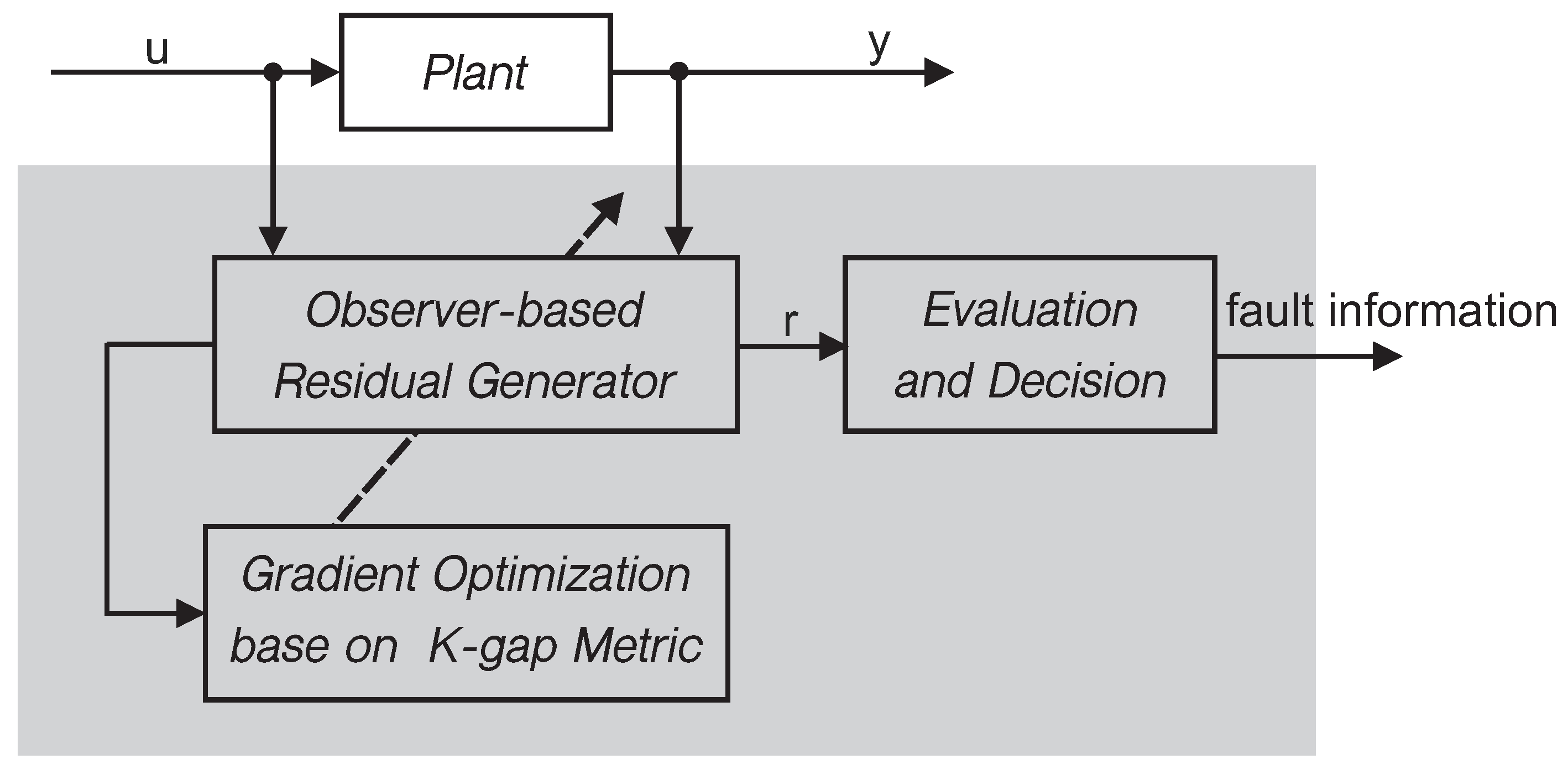
Considering that practical circumstance and industrial environment may change, the fault detection by the offline designed residual generator cannot satisfy the complicated industrial demand. In this section, a novel real-time configuration scheme for residual generators is proposed, which is essentially an optimization algorithm based on the K-gap metric. To be specific, an observer-based residual generator is constructed and the gradient optimization algorithm is used to update its parameters. Thus, the real-time configuration is achieved for the observer-based residual generators, the framework of which is displayed in Figure 1 for clarification.

3.1. The Observer-Based General Generator

For the discrete-time LTI system (1), a full-order state observer is constructed with the minimal state-space representation as
x o ( k + 1 ) = A o x o k + B o u k + L o y k ,
r k = C o x o k + D o u k + y k ,
where x o k R n indicates the state of the full-order observer and r k R m stands for the residual vector. A o , B o , C o , D o , L o are observer matrices with proper dimensions.
For observer (9) and (10), a similarity transformation is performed by x o = T ν x ν , which yields
x ν ( k + 1 ) = A ν x ν k + B ν u k + L ν y k ,
r k = C ν x ν k + D ν u k + y k ,
where A ν = T ν 1 A o T ν , B ν = T ν 1 B o , L ν = T ν 1 L o , C ν = C o T ν , D ν = D o . According to the authors of [40], the controllability Gramian matrix of systems (11) and (12) is equivalent to the identity matrix, i.e.,
A ν A ν T + B ν B ν T = I n ,
which gives rise to a column-orthogonal matrix B ν T A ν T . Consequently, there exists an invertible matrix Ψ such that
B ν T A ν T = Ψ 0 I n .
Referring to the literature [41], the parameterization based on the input normal form can be described by
B ν T θ A B A ν T θ A B = Ψ 1 θ A B 1 Ψ n l θ A B n l 0 I n ,
in which θ A B R n l and its entries take values in the range ( 1 , 1 ) . By introducing the following form for each parameter θ A B i , i = 1 , , n l
U θ A B i = θ A B i 1 θ A B 2 i 1 θ A B 2 i θ A B i ,
the matrices Ψ i θ A B i , i = 1 , , n l are represented as
Ψ 1 θ A B 1 = I n 1 0 0 0 U θ A B 1 0 0 0 I l 1 , Ψ n l θ A B n l = I l 1 0 0 0 U θ A B n l 0 0 0 I n 1 .
As the parameterization of the input normal form is on the basis of the asymptotic stability, no additional restriction on the parameter space is needed, which is a significant advantage of this transformation.
Then, the procedure to obtain the SKR corresponding to the observer (11) is given as below. It is obvious from Formula (12) that
r k s = C ν x ν k s + D ν u k s + y k s .
Subsequently,
r k s + 1 = C ν x ν k s + 1 + D ν u k s + 1 + y k s + 1 = C ν A ν x ν k s + B ν u k s + L ν y k s + D ν u k s + 1 + y k s + 1 = C ν A ν x ν k s + C ν B ν u k s + D ν u k s + 1 + C ν L ν y k s + y k s + 1 , r k s + 2 = C ν x ν k s + 2 + D ν u k s + 2 + y k s + 2 = C ν A ν x ν k s + 1 + B ν u k s + 1 + L ν y k s + 1 + D ν u k s + 2 + y k s + 2 = C ν A ν A ν x ν k s + B ν u k s + L ν y k s + C ν B ν u k s + 1 + C ν L ν y k s + 1 + D ν u k s + 2 + y k s + 2 = C ν A ν 2 x ν k s + C ν A ν B ν u k s + C ν B ν u k s + 1 + D ν u k s + 2 + C ν A ν L ν y k s + C ν L ν y k s + 1 + y k s + 2 , r k s + 3 = C ν x ν k s + 3 + D ν u k s + 3 + y k s + 3 = C ν A ν x ν k s + 2 + B ν u k s + 2 + L ν y k s + 2 + D ν u k s + 3 + y k s + 3 = C ν A ν A ν x ν k s + 1 + B ν u k s + 1 + L ν y k s + 1 + C ν B ν u k s + 2 + C ν L ν y k s + 2 + D ν u k s + 3 + y k s + 3 = C ν A ν 2 A ν x ν k s + B ν u k s + L ν y k s + C ν A ν B ν u k s + 1 + C ν A ν L ν y k s + 1 + C ν B ν u k s + 2 + C ν L ν y k s + 2 + D ν u k s + 3 + y k s + 3 = C ν A ν 3 x ν k s + C ν A ν 2 B ν u k s + C ν A ν B ν u k s + 1 + C ν B ν u k s + 2 + D ν u k s + 3 + C ν A ν 2 L ν y k s + C ν A ν L ν y k s + 1 + C ν L ν y k s + 2 + y k s + 3 ,
which implies
r k = C ν A ν s x ν k s + C ν A ν s 1 B ν u k s + + C ν B ν u k 1 + D ν u k + C ν A ν s 1 L ν y k s + + C ν L ν y k 1 + y k .
Then, it is easy to obtain that
r s k = Γ s x ν k s + H u , s u s k + H y , s y s k ,
where
Γ s = C ν C ν A ν C ν A ν s , H u , s = D ν 0 0 C ν B ν 0 0 C ν A ν s 1 B ν C ν B ν D ν , H y , s = I 0 0 C ν L ν 0 0 C ν A ν s 1 L ν C ν L ν I .
Then, the following equation is obtained:
R k , s = Γ s X ν , k s + H u , s U k , s + H y , s Y k , s .
As C ν A ν s 0 , s , according to Definition 3, the SKR corresponding to the state observer can be obtained by the equation
K o , s = H u , s H y , s = D ν 0 0 I 0 0 C ν B ν 0 0 C ν L ν 0 0 C ν A ν s 1 B ν C ν B ν D ν C ν A ν s 1 L ν C ν L ν I
with removing the front finite rows to eliminate the influence of past data. By applying the singular value decomposition to K o , s , it holds that
K o , s = U Σ 1 0 V 1 T V 2 T
and thus, the normalized SKR is
K ¯ o , s = V 1 T .

3.2. Online Gradient Optimization

Based on the above observer-based residual generator, this subsection will establish an gradient optimization method for the real-time configuration by taking advantage of the K-gap metric between the observer and system plant.
Define
θ = θ A B θ C ν θ D ν θ L ν = θ A B v e c ( C ν ) v e c ( D ν ) v e c ( L ν ) ,
and denote θ i ( i = 1 , 2 , , τ = n l + 2 m n + m l ) as the i-th term of θ .
The optimization problem is described by
minimize J = δ k d , s K o , s , K d , s , subject to θ S ,
where K d , s , K o , s are, respectively, the SKRs of the system (1) and the observer (11), and S is the set in which the entries of any vector belong to ( 1 , 1 ) . To achieve the minimization of cost function J, the Taylor expansion of cost function J at the j-th iteration is considered
J θ ( j ) ( j ) = J θ ( j 1 ) ( j ) + J θ ( j ) ( j ) θ ( j ) | θ ( j 1 ) T θ ( j ) θ ( j 1 ) + 1 2 θ ( j ) θ ( j 1 ) T 2 J θ ( j ) ( j ) θ ( j ) θ ( j ) T | θ ( j 1 ) θ ( j ) θ ( j 1 ) + o 3 θ ( j ) θ ( j 1 ) ,
where J θ ( j ) ( j ) θ ( j ) and 2 J θ ( j ) ( j ) θ ( j ) θ ( j ) T denote the gradient and the Hessian matrix of cost function J, respectively. o 3 · stands for the infinitesimal of order higher than 3. Regardless of the high-order infinitesimal, a necessary condition to minimize the function J θ ( j ) ( j ) is to command
J θ ( j ) ( j ) θ ( j ) | θ ( j 1 ) + 2 J θ ( j ) ( j ) θ ( j ) θ ( j ) T | θ ( j 1 ) θ ( j ) θ ( j 1 ) = 0 .
Rewriting the expression (17) gives the iteration procedure of updating the parameter θ as
θ ( j ) = θ ( j 1 ) 2 J θ ( j ) ( j ) θ ( j ) θ ( j ) T | θ ( j 1 ) 1 J θ ( j ) ( j ) θ ( j ) | θ ( j 1 ) ,
which is the Gauss–Newton iteration widely used in the literature. However, this method requires the invertibility of 2 J θ ( j ) ( j ) θ ( j ) θ ( j ) T | θ ( j 1 ) and may lead to a heavy computational burden. To improve its applicability in numerical computation, an iteration procedure known as the steepest-descent algorithm is introduced
θ ( j ) = θ ( j 1 ) Δ ( j ) J θ ( j ) ( j ) θ ( j ) | θ ( j 1 ) ,
where Δ ( j ) > 0 is a diagonal matrix meaning the step length of the j-th iteration.
Clearly, the key question of the optimization is to calculate the gradient J θ = δ k d , s K o , s , K d , s θ .
It is obtained from Lemma 2 that
δ k d , s K o , s , K d , s θ = σ ¯ I K ¯ d , s T K ¯ d , s K ¯ o , s T K ¯ o , s θ = e i g ¯ I K ¯ d , s T K ¯ d , s K ¯ o , s T K ¯ o , s K ¯ o , s T K ¯ o , s I K ¯ d , s T K ¯ d , s θ = e i g ¯ I K ¯ d , s T K ¯ d , s K ¯ o , s T K ¯ o , s I K ¯ d , s T K ¯ d , s θ = 1 2 δ k d , s K o , s , K d , s e i g ¯ I K ¯ d , s T K ¯ d , s K ¯ o , s T K ¯ o , s I K ¯ d , s T K ¯ d , s θ = 1 2 δ k d , s K o , s , K d , s e i g ¯ I K ¯ d , s T K ¯ d , s K ¯ o , s T K ¯ o , s I K ¯ d , s T K ¯ d , s θ 1 e i g ¯ I K ¯ d , s T K ¯ d , s K ¯ o , s T K ¯ o , s I K ¯ d , s T K ¯ d , s θ 2 e i g ¯ I K ¯ d , s T K ¯ d , s K ¯ o , s T K ¯ o , s I K ¯ d , s T K ¯ d , s θ i e i g ¯ I K ¯ d , s T K ¯ d , s K ¯ o , s T K ¯ o , s I K ¯ d , s T K ¯ d , s θ τ .
Denote ξ as the eigenvector corresponding to the maximum eigenvalue of matrix I K ¯ d , s T K ¯ d , s K ¯ o , s T K ¯ o , s I K ¯ d , s T K ¯ d , s and focus on the partial derivative on the i-th variable, i.e.,
e i g ¯ I K ¯ d , s T K ¯ d , s K ¯ o , s T K ¯ o , s I K ¯ d , s T K ¯ d , s θ i = ξ T I K ¯ d , s T K ¯ d , s K ¯ o , s T K ¯ o , s I K ¯ d , s T K ¯ d , s ξ θ i = ξ T I K ¯ d , s T K ¯ d , s K ¯ o , s T K ¯ o , s I K ¯ d , s T K ¯ d , s θ i ξ = ξ T I K ¯ d , s T K ¯ d , s K ¯ o , s T K ¯ o , s θ i I K ¯ d , s T K ¯ d , s ξ .
Making use of the result of singular value decomposition in (16) gives
K ¯ o , s T K ¯ o , s = V 1 V 1 T = v 1 v 1 T + v 2 v 2 T + + v μ v μ T ,
where V 1 = v 1 v 2 v μ and μ means the row number of matrix K ¯ o , s . Therefore,
K ¯ o , s T K ¯ o , s θ i = v 1 v 1 T + v 2 v 2 T + + v μ v μ T θ i = α = 1 μ v α v α T θ i ,
in which
v α v α T θ i = v α θ i v α T + v α v α T θ i = v α θ i v α T + v α v α θ i T .
Notice that
K o , s T K o , s = V 1 V 2 Σ 1 T 0 U T U Σ 1 0 V 1 T V 2 T = V 1 V 2 Σ 1 2 0 0 0 V 1 T V 2 T ,
where Σ 1 = d i a g { σ 1 , σ 2 , , σ μ } . As a result, v α is the eigenvector corresponding to the i-th eigenvalue of matrix K o , s T K o , s . For any α = 1 , 2 , , μ , i = 1 , 2 , , τ ,
v α θ i = σ α 2 I K o , s T K o , s + K o , s T K o , s v α θ i = σ α 2 I K o , s T K o , s + K o , s T K o , s θ i v α .
It can be easily obtained that
K o , s T K o , s θ i = K o , s T θ i K o , s + K o , s T K o , s θ i = K o , s θ i T K o , s + K o , s T K o , s θ i .
Substituting the Formula (15) into the partial derivative leads to
K o , s θ i = D ν 0 0 I 0 0 C ν B ν 0 0 C ν L ν 0 0 C ν A ν s 1 B ν C ν B ν D ν C ν A ν s 1 L ν C ν L ν I θ i .
As θ i may be one element of any vector of θ A B , θ C ν , θ D ν , θ L ν , the deduction will be divided into four cases in the following.
First, when the parameter θ i is one element of vector θ A B ,
K o , s θ A B i = H u , s θ A B i H y , s θ A B i ,
where
H u , s θ A B i = 0 0 0 C ν B ν θ A B i 0 0 C ν A ν θ A B i B ν + A ν B ν θ A B i C ν B ν θ A B i 0 C ν A ν s 1 θ A B i B ν + A ν s 1 B ν θ A B i C ν A ν s 2 θ A B i B ν + A ν s 2 B ν θ A B i C ν B ν θ A B i , H y , s θ A B i = 0 0 0 0 0 0 C ν A ν θ A B i L ν 0 0 C ν A ν s 1 θ A B i L ν C ν A ν s 2 θ A B i L ν 0 ,
and
B ν T θ A B A ν T θ A B θ A B i = B ν T θ A B θ A B i A ν T θ A B θ A B i = Ψ 1 θ A B 1 Ψ i θ A B i θ A B i Ψ n l θ A B n l 0 I n , Ψ i θ A B i θ A B i = 0 0 0 0 U θ A B i θ A B i 0 0 0 0 , U θ A B i θ A B i = 1 θ A B i 1 θ A B 2 i θ A B i 1 θ A B 2 i 1 .
Second, when the parameter θ i is one element of vector θ C ν , assume θ i = c p q , p { 1 , 2 , , m } , q { 1 , 2 , , n } , where c p q corresponds to the p-th row and the q-th column of matrix C ν ,
D ν 0 0 I 0 0 C ν B ν 0 0 C ν L ν 0 0 C ν A ν s 1 B ν C ν B ν D ν C ν A ν s 1 L ν C ν L ν I c p q = 0 0 0 0 0 0 0 C ν c p q B ν 0 C ν c p q L ν 0 0 0 C ν c p q A ν B ν C ν c p q B ν C ν c p q A ν L ν C ν c p q L ν 0 0 C ν c p q A ν s 1 B ν C ν c p q A ν s 2 B ν C ν c p q B ν 0 C ν c p q A ν s 1 L ν C ν c p q A ν s 2 L ν C ν c p q L ν 0
with
C ν c p q = c 11 c 1 q c 1 n c p 1 c p q c p n c m 1 c m q c m n c p q = 0 0 0 0 1 0 0 0 0 .
Third, when the parameter θ i is one element of vector θ D ν , assume θ i = d p q , p { 1 , 2 , , m } , q { 1 , 2 , , l } , where d p q corresponds to the p-th row and the q-th column of matrix D ν ,
D ν 0 0 I 0 0 C ν B ν 0 0 C ν L ν 0 0 C ν A ν s 1 B ν C ν B ν D ν C ν A ν s 1 L ν C ν L ν I d p q = D ν d p q 0 0 0 0 0 0 D ν d p q 0 0 0 0 0 D ν d p q 0 0 0 0 0 0 D ν d p q 0 0
with
D ν d p q = d 11 d 1 q d 1 l d p 1 d p q d p l d m 1 d m q d m l d p q = 0 0 0 0 1 0 0 0 0 .
Fourth, when the parameter θ i is one element of vector θ L ν , assume θ i = l p q , p { 1 , 2 , , n } , q { 1 , 2 , , m } , where l p q corresponds to the p-th row and the q-th column of matrix L ν ,
D ν 0 0 I 0 0 C ν B ν 0 0 C ν L ν 0 0 C ν A ν s 1 B ν C ν B ν D ν C ν A ν s 1 L ν C ν L ν I l p q = 0 0 0 0 0 0 0 C ν L ν l p q 0 0 0 C ν A ν L ν l p q C ν L ν l p q 0 0 0 0 0 C ν A ν s 1 L ν l p q C ν L ν l p q 0
with
L ν l p q = l 11 l 1 q l 1 m l p 1 l p q l p m l n 1 l n q l n m l p q = 0 0 0 0 1 0 0 0 0 .
Up to now, the optimization problem is solved and the parameter optimization is derived by the above deduction. To summarize, this study aims to achieve the online configuration of an observer-based residual generator for fault detection systems. To achieve this, the observer is first transformed into the input normal form, which guarantees the asymptotic stability. Based on the input normal form, the residual generator is established, and the purpose is to online configure its parameters to cope with the operation condition changes or uncertainties of the system. Then, the optimization configuration strategy is taken into account and the optimization problem is proposed by utilizing the K-gap metric concept. By employing the gradient descent method, the parameter configuration is finally obtained for the online configuration realization.
Remark 1.
Note that the optimization problem of this paper is established based on the K-gap metric concept. The purpose is to minimize the K-gap metric δ k d , s K o , s , K d , s between the observer and system plant, which characterizes the distance between two kernel subspaces. Referring to the work in [37], a definition of cluster is described as below. For δ f ( 0 , 1 ) , the set
C f { K : δ k K , K f δ f }
is called C f cluster with the cluster center K f and cluster radius δ f . From this point of view, by minimizing the K-gap metric δ k d , s K o , s , K d , s , the obtained K o , s falls into the cluster with the cluster center K d , s and a certain cluster radius. A smaller cluster radius contributes to a more similar level of K o , s to K d , s . Therefore, the residual generator based on the optimized K o , s can guarantee the reliability and efficiency of the fault detection system.

3.3. Online Configuration Realization of Fault Detection

This subsection will present an online algorithm to achieve the fault detection goal by employing the newly proposed gradient configuration scheme. The detailed procedure of online configuring the observer-based residual generator is described in Algorithm 1 as follows.
Algorithm 1 Online Configuration of Observer-Based Residual Generator
Step 1:    Collect the I/O data u ( k ) , y ( k ) at each k and select an iteration interval W
Step 2:    Execute Step 3–6 for the j-th iteration every W
Step 3:    According to Definition 3, compute the SKR K d , s and its normalized result K ¯ d , s
Step 4:    Compute the SKR K o , s and its normalized result K ¯ o , s corresponding to the observer
    by (15) and (16)
Step 5:    Apply Lemma 2 to obtain the K-gap metric δ k d , s K o , s , K d , s between K o , s and K d , s
Step 6:    Given a scalar ε , if δ k d , s K o , s , K d , s > ε , compute the gradient and update the parameters
    of residual generator according to (19), increase j by 1 and return Step 2, otherwise
    the configuration ends
To achieve the fault detection, the evaluation function is set to be J ( k ) = r ( k ) 2 2 with the threshold J t h chosen as below,
J t h = sup f = 0 , d , Δ J ( k ) ,
where d and Δ represent the disturbance and model uncertainties, respectively. Based on the online residual generator obtained by Algorithm 1, calculate the evaluation function J ( k ) . The decision logic is described by
J ( k ) > J t h faulty , J ( k ) J t h fault-free .

4. Simulation Experiment

In this section, a simulation experiment is carried out on a three-tank system plant to show the effectiveness and advantages of the proposed real-time configuration scheme. 
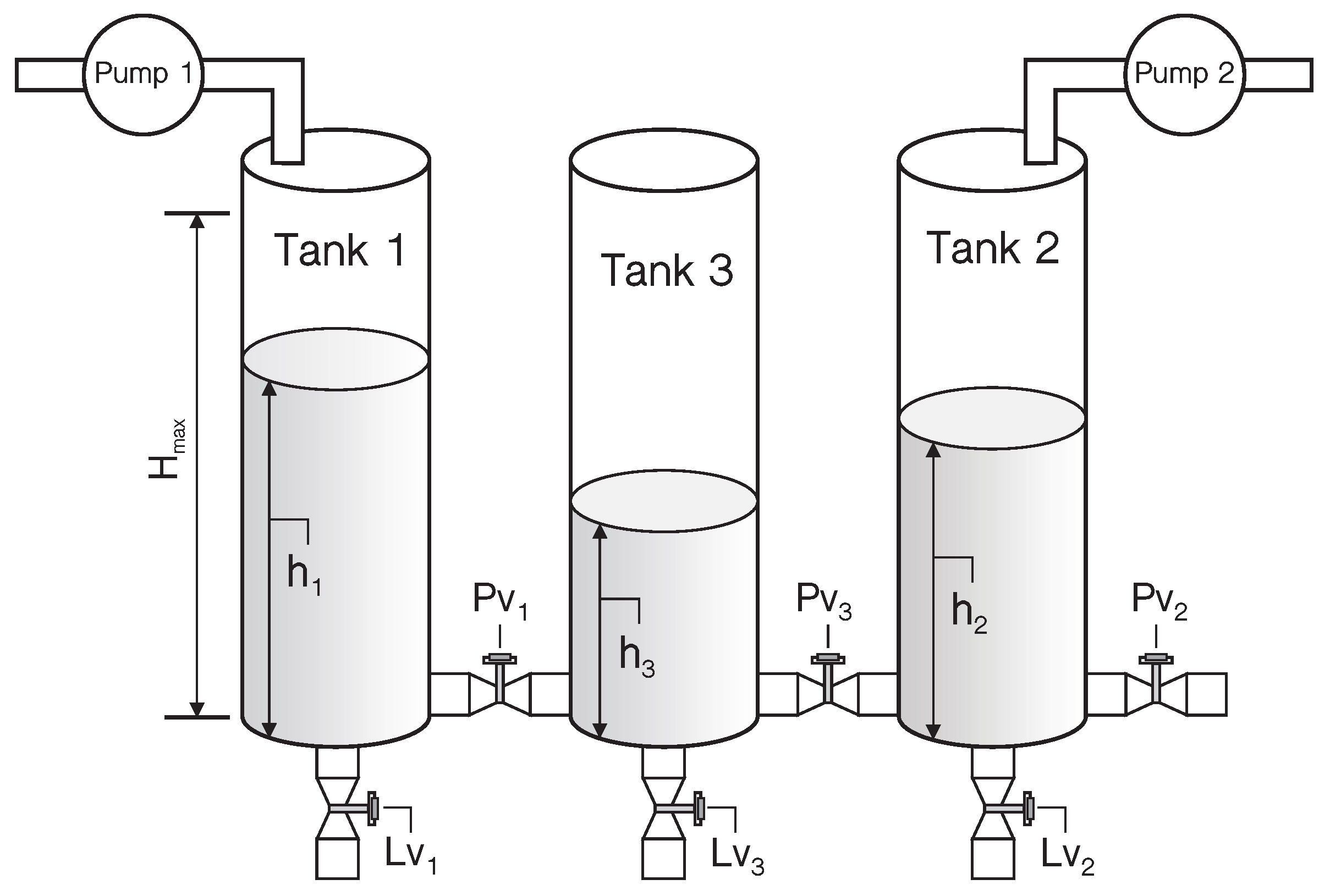
Figure 2 shows the schematic diagram of the three-tank system, which is composed of three water tanks and some connecting pipes. In Figure 2, h 1 , h 2 , and h 3 refer to the water levels of the three tanks, which are measurable through sensors and deemed as the output signals. Q 1 and Q 2 stand for the incoming mass flow rates of Pump 1 and Pump 2 and are used as the input signals. Besides, PV 1 , PV 2 , PV 3 , LV 1 , LV 2 , LV 3 are the adjustable ball valves to administrate the opening and closing of these pipes.
The system plant can be represented by the nonlinear dynamics
A h ˙ 1 = Q 1 α 1 s s g n ( h 1 h 3 ) 2 g | h 1 h 3 | , A h ˙ 2 = Q 2 + α 3 s s g n ( h 3 h 2 ) 2 g | h 3 h 2 | α 2 s 2 g h 2 , A h ˙ 3 = α 1 s s g n ( h 1 h 3 ) 2 g | h 1 h 3 | α 3 s s g n ( h 3 h 2 ) 2 g | h 3 h 2 | ,
in which A = 154 cm 2 and s = 0.5 cm 2 denote the cross section area of the tanks and pipes, respectively, and α 1 = 0.46 , α 2 = 0.60 , α 3 = 0.45 successively indicate the coefficients of flow for the three pipes. In addition, the maximum height of the tanks is chosen as H m a x = 62 cm, and the maximum flow rates of pumps 1 and 2 are set to be Q 1 m a x = Q 2 m a x = 100 cm 3 /s. For certain operation points, the nonlinear representation (21) can be reformulated into the LTI system (1) by utilizing the linearization technique.
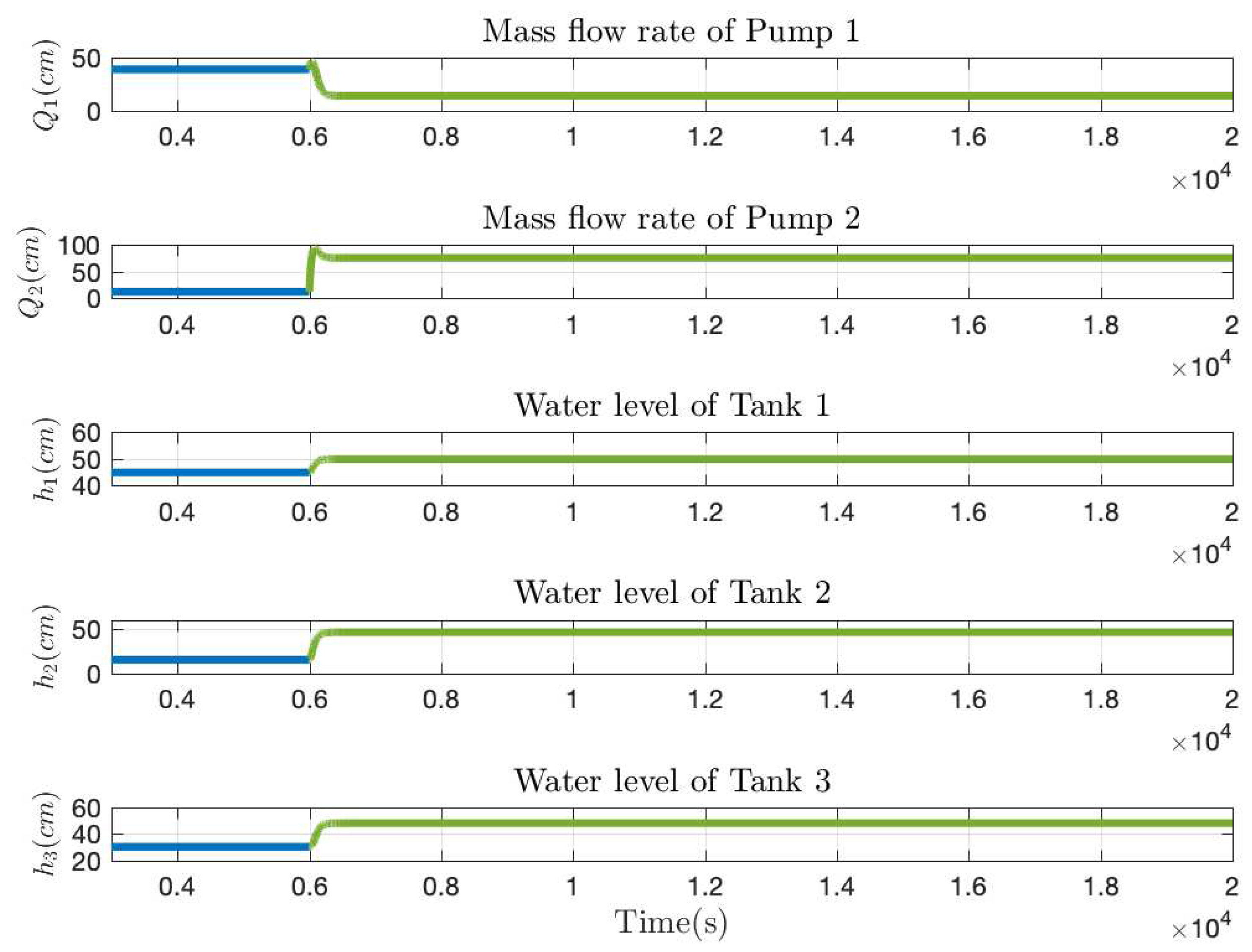
In this simulation, the operating time is set to be 25,000 s and the sampling period is chosen as 1s. At first, the operation point of the three-tank system is considered to be h 1 = 45 cm, h 2 = 15 cm, and h 3 = 30 cm, for which a residual generator is predesigned and applied in the fault detection process. Due to the demand of practical industry, it is supposed that the operation point changes to h 1 = 50 cm, h 2 = 46 cm and h 3 = 48 cm at 6000 s. The process data are collected and displayed in Figure 3.
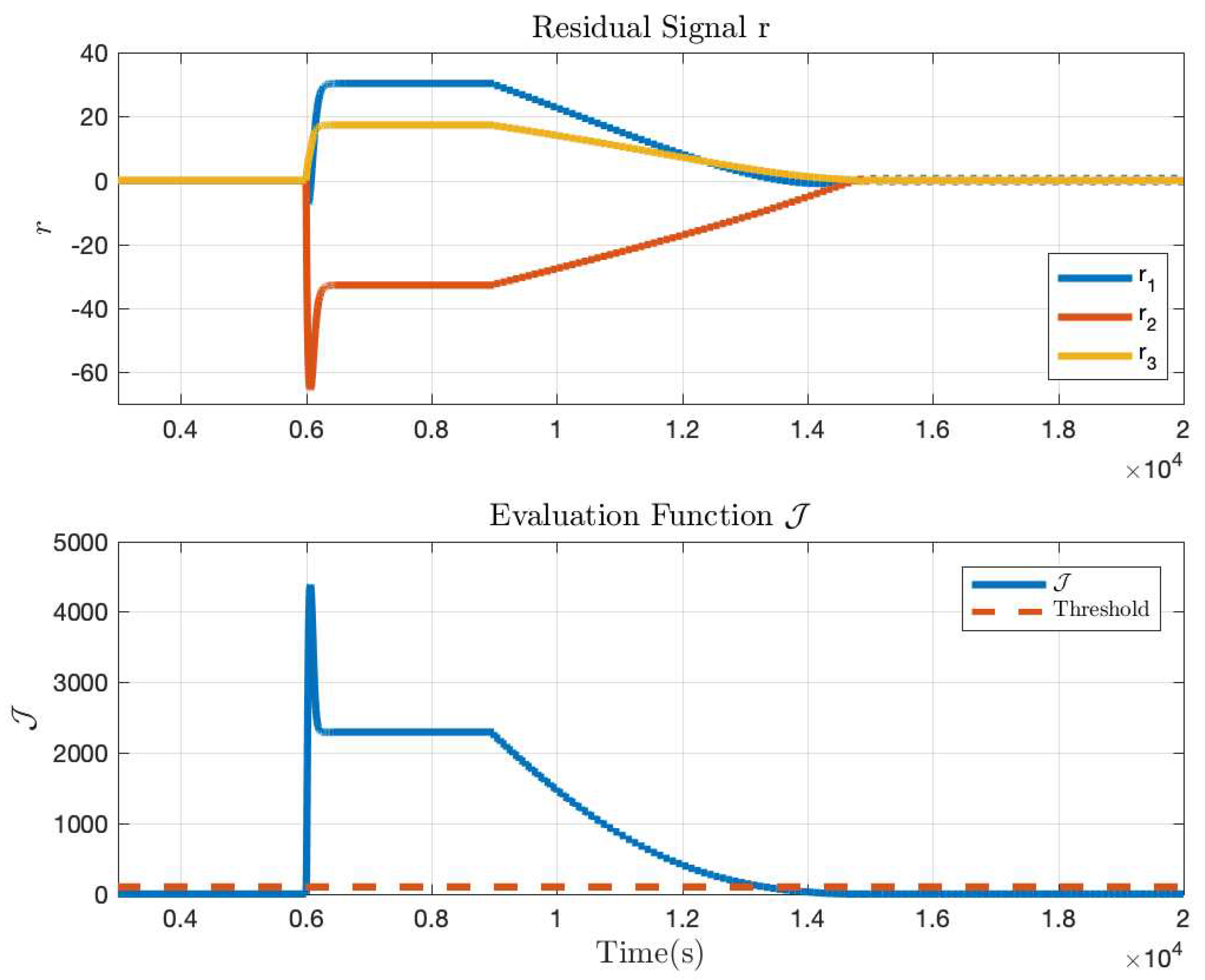
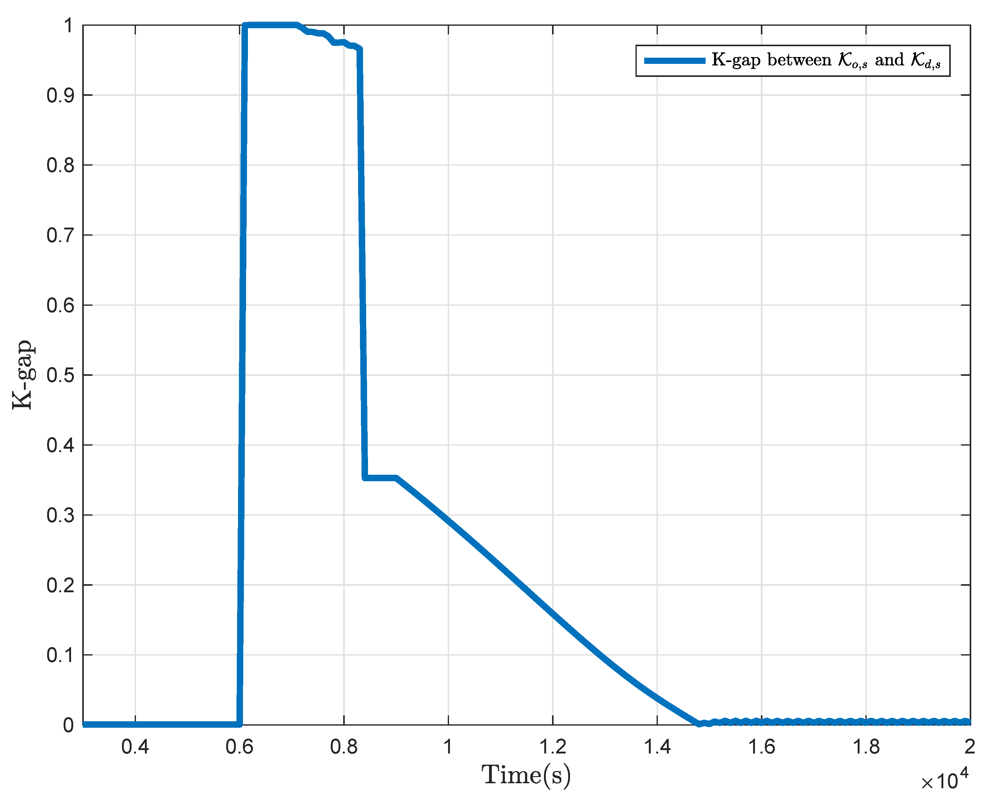
Figure 4 displays the evolution curves of residual signals and evaluation function and Figure 5 exhibits the K-gap metric between system plant and observer. Before the change of the operation point at 6000 s, the evaluation function value is lower than the threshold and the K-gap metric value is 0.0007072 , which means the kernel subspaces of system plant and observer are sufficiently close and thus the predesigned residual generator is proper. From 6000 s, the value of evaluation function increases and obviously exceeds the threshold, which causes a false alarm under the circumstance of no fault. Meanwhile, the K-gap metric between system plant and observer becomes enormous. Clearly, the predesigned residual generator is no more applicable for the system with a changed operation point. To handle this problem and demonstrate the validity of the proposed real-time configuration method, the real-time configuration algorithm, i.e., Algorithm 1 is implemented at 9000 s. It can be observed from Figure 4 and Figure 5 that from 9000 s, the K-gap metric value begins to decline as the real-time configuration implementation, and the values of residual signal and evaluation function, begin to decrease and gradually converge. At ~14,700 s, the K-gap metric settles at ~ 0.001 
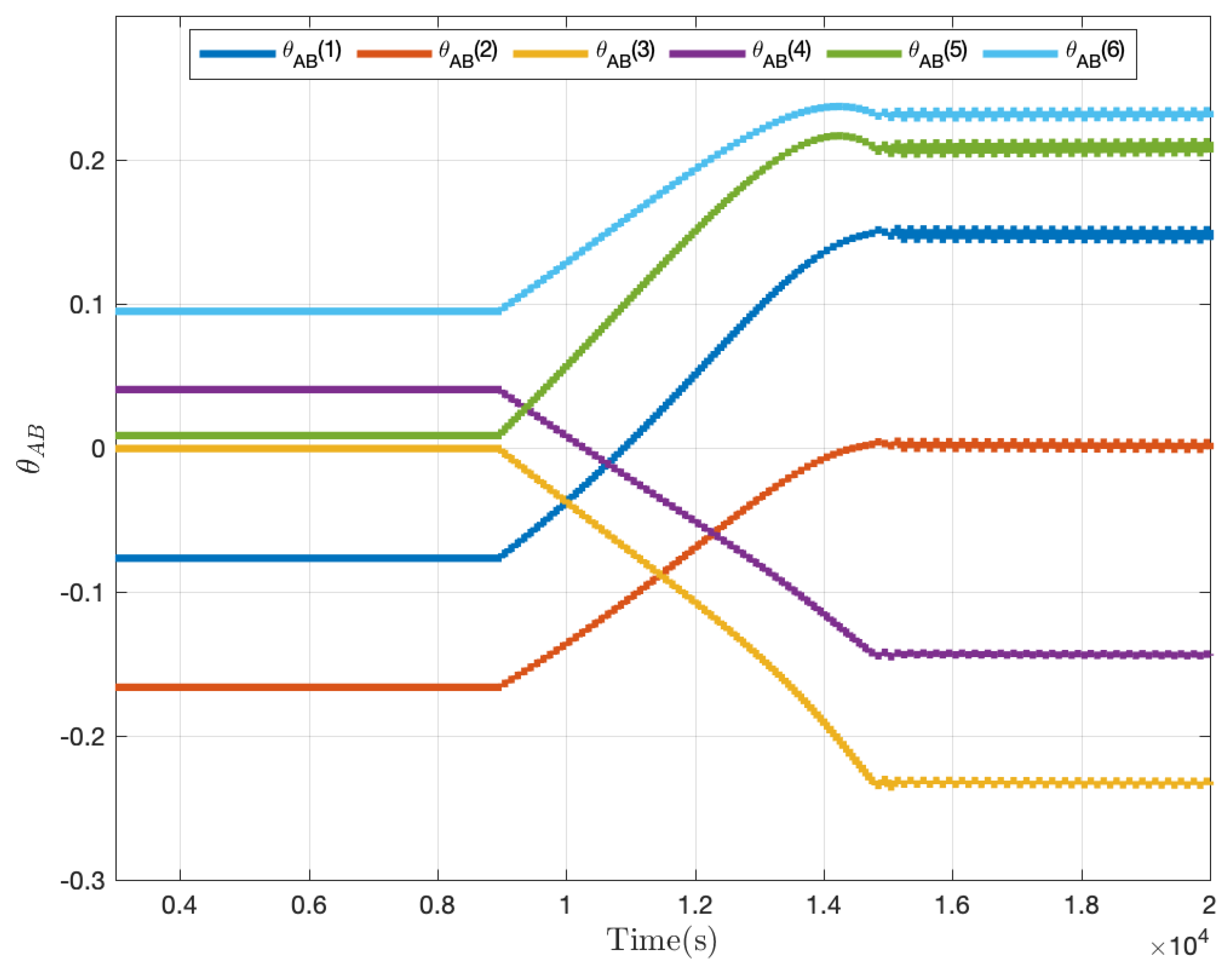
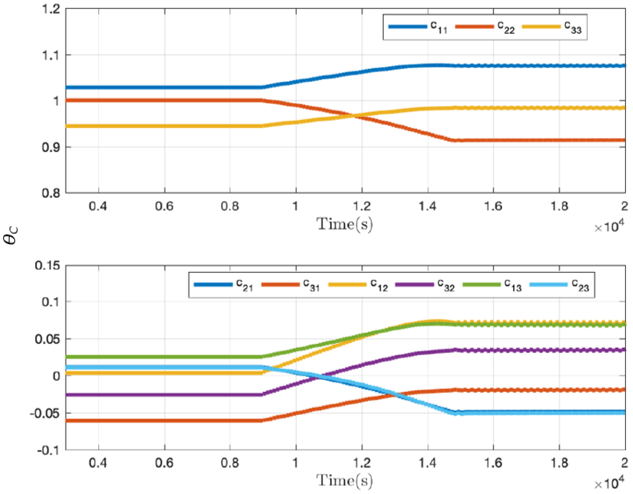
and the kernel subspace of observer is adequately approximate to the kernel subspace of system plant. In addition, the value of evaluation function becomes less than the threshold and the false alarm disappears, which reflects that the real-time optimized residual generator is effective for the current operation point. Therefore, the optimization goal is realized and the real-time configuration of the residual generator is achieved for the system. In addition, the optimized parameters of θ A B , θ C are, respectively, given in Figure 6 and Figure 7 to show the parameter configuration process.
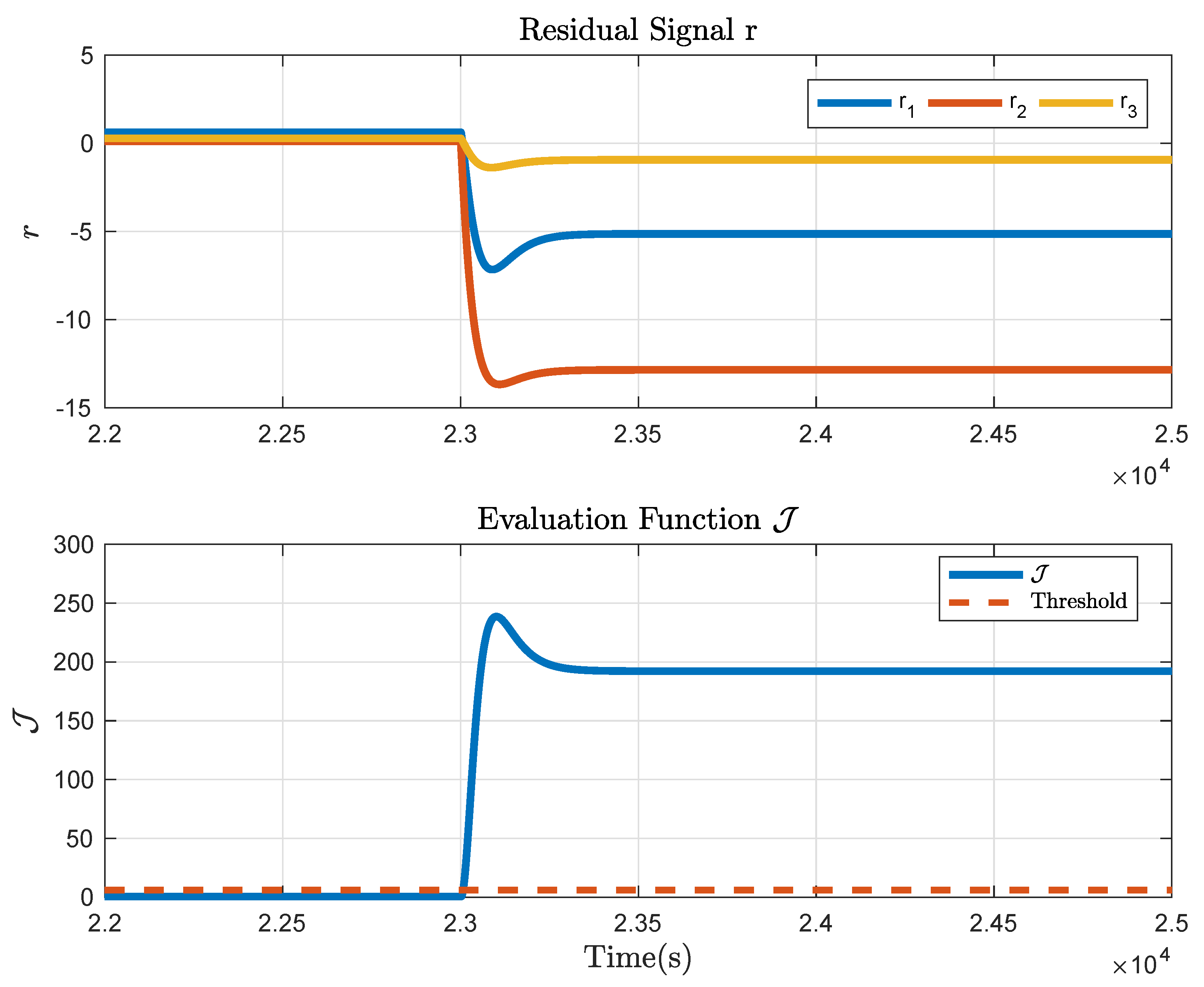
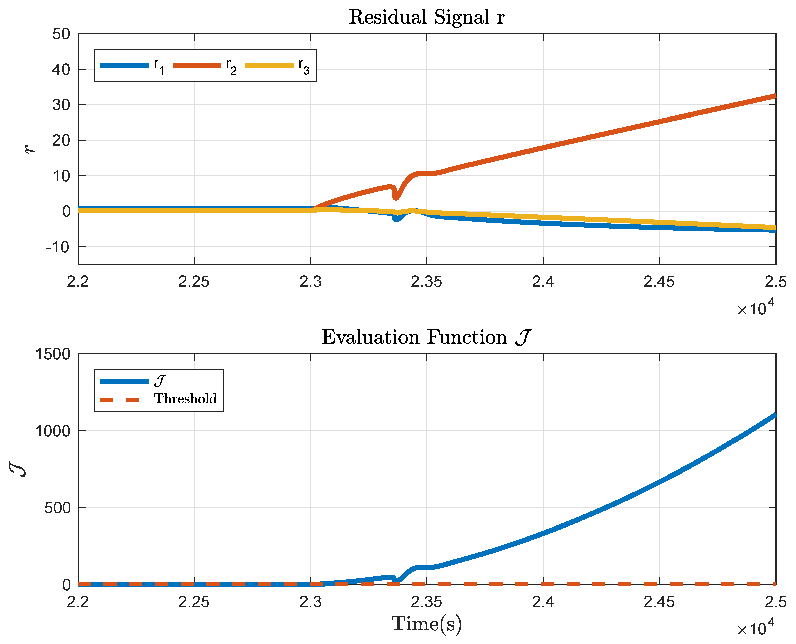
Now, the online configured residual generator is applied to the fault detection implementation to verify its usefulness. Here, two types of fault will be considered and assumed to happen at 23,000 s, respectively. First, consider that a leakage fault happens in the tank 2 with a 20% leakage level at 23,000 s. Figure 8 shows the fault detection result by the online configured residual generator. It can be seen from the figure that the value of the evaluation function exceeds the threshold at 23,005 s, which means that the leakage fault is detected. Then, the usefulness of the fault detection based on the online configuration scheme is illustrated. Moreover, another type of fault, i.e., a drift fault with slope 0.01 occurring in the sensor of water level of tank 2, is considered at 23,000 s. Figure 9 shows the corresponding fault detection result, from which one can see that the drift fault is detected by the proposed optimization configuration algorithm at 23,042 s. According to the above fault detection results, it is clear that the optimization configuration method of this paper can detect the fault accurately and timely. As a consequence, the real-time configuration method proposed in this paper can effectively deal with the system under the influence of operation point changes or uncertainties, and the effectiveness of the method in fault detection implementation is demonstrated.

5. Conclusions

Considering that the changes of operating conditions, practical environment, and some uncertainties may occur in industrial processes, this paper is dedicated to the real-time configuration design for fault detection systems. As an important means of real-time configuration, the gradient optimization scheme is considered and adopted in this work for the real-time configuration implementation. A novel optimization algorithm is developed by virtue of the gradient-based technique, in which the K-gap metric between the residual generator and the current system is minimized. Then, the residual generator parameters can be updated based on the I/O data, and the real-time configuration for fault detection systems is realized to satisfy a particular demand. Finally, the usefulness and merits of the proposed approach are demonstrated through the benchmark case on a three-tank model. One main advantage of this work is that by virtue of the K-gap metric technique together with the gradient-based method, the online-configured residual generator parameters are reliable to guarantee the fault detection performance for industrial systems with changeable operating points. Besides, the input/output data information are sufficiently exploited for the fault detection implementation, which avoids the difficulties of the system identification in practice. As the real-time configuration method is carried out based on the process data, the computation amount would be the main concern of the implementation, especially for large-scale industrial systems, which inspires us to conduct further research in this field. Note that one of the main contributions of this paper is to introduce the K-gap idea into the real-time configuration implementation, which exploits the essential characteristic of fault detection systems. In our future work, the K-gap-based optimization configuration approach will be further extended to systems with nonlinearities and fault-tolerant control issues.

Author Contributions

Conceptualization, H.Z.; Formal analysis, T.L.; Funding acquisition, H.L.; Methodology, H.Z.; Software, H.Z.; Supervision, H.L.; Writing—original draft, H.Z.; Writing—review & editing, H.L. All authors have read and agreed to the published version of the manuscript.

Funding

This work is supported by National Natural Science Foundation of China under Grant U20A20186, 62073104.

Institutional Review Board Statement

Not applicable.

Informed Consent Statement

Not applicable.

Data Availability Statement

Not applicable.

Conflicts of Interest

The authors declare no conflict of interest.

References

  1. Fekih, A.; Xu, H.; Chowdhury, F. Neural networks based system identification techniques for model based fault detection of nonlinear systems. Int. J. Innov. Comput. Inf. Control 2007, 3, 1073–1085. [Google Scholar]
  2. Wang, X.L.; Yang, G.H. Event-triggered fault detection for discrete-time T-S fuzzy systems. ISA Trans. 2018, 76, 18–30. [Google Scholar] [CrossRef] [PubMed]
  3. Son, J.; Du, Y. Model-based stochastic fault detection and diagnosis of Lithium-Ion batteries. Processes 2019, 7, 38. [Google Scholar] [CrossRef] [Green Version]
  4. Mazzoletti, M.A.; Bossio, G.R.; De Angelo, C.H.; Espinoza-Trejo, D.R. A Model-based strategy for interturn short-circuit fault diagnosis in PMSM. IEEE Trans. Ind. Electron. 2017, 64, 7218–7228. [Google Scholar] [CrossRef]
  5. Huang, S.P.; Xiang, Z.R.; Karimi, H.R. Mixed L/L1 fault detection filter design for fuzzy positive linear systems with time-varying delays. IET Control Theory A 2014, 8, 1023–1031. [Google Scholar] [CrossRef]
  6. Poon, J.; Jain, P.; Konstantakopoulos, I.; Spanos, C.; Panda, S.; Sanders, S. Model-based fault detection and identification for switching power converters. IEEE Trans. Power Electron. 2017, 32, 1419–1430. [Google Scholar] [CrossRef]
  7. Yang, C.; Fang, H. A new nonlinear model-based fault detection method using Mann-Whitney test. IEEE Trans. Ind. Electron. 2020, 67, 10856–10864. [Google Scholar] [CrossRef]
  8. Gao, Y.; Xiao, F.; Liu, J.; Wang, R. Distributed soft fault detection for interval type-2 fuzzy-model-based stochastic systems with wireless sensor networks. IEEE Trans. Ind. Inform. 2019, 15, 334–347. [Google Scholar] [CrossRef]
  9. Zhou, S.; Bai, J.; Wu, F. Decentralized fault detection and fault-tolerant control for nonlinear interconnected systems. Processes 2021, 9, 591. [Google Scholar] [CrossRef]
  10. Zhang, P.; Ding, S.X.; Wang, G.Z.; Zhou, D.H. Fault detection of linear discrete-time periodic systems. IEEE Trans. Automat. Control 2005, 50, 239–244. [Google Scholar] [CrossRef]
  11. Zhong, M.; Ding, S.X.; Ding, E.L. Optimal fault detection for linear discrete time-varying systems. Automatica 2010, 46, 1395–1400. [Google Scholar] [CrossRef]
  12. Li, X.; Yang, G.H. Fault detection for linear stochastic systems with sensor stuck faults. Optim. Contr. Appl. Met. 2012, 33, 61–80. [Google Scholar] [CrossRef]
  13. Su, Q.Y.; Li, J. Fault detection for a class of uncertain linear systems. Math. Probl. Eng. 2013, 33, 856914. [Google Scholar] [CrossRef]
  14. Fan, C.; Lam, J.; Xie, X. Fault detection observer design for periodic piecewise linear systems. Int. J. Syst. Sci. 2020, 51, 1622–1636. [Google Scholar] [CrossRef]
  15. Li, L.; Ding, S.X.; Qiu, J.; Yang, Y.; Xu, D. Fuzzy observer-based fault detection design approach for nonlinear processes. IEEE Trans. Syst. Man Cybern. Syst. 2017, 47, 1941–1952. [Google Scholar] [CrossRef]
  16. Li, L.; Ding, S.X.; Yang, Y.; Zhang, Y. Robust fuzzy observer-based fault detection for nonlinear systems with disturbances. Neurocomputing 2016, 174, 767–772. [Google Scholar] [CrossRef]
  17. Zhirabok, A.; Shumsky, A.; Solyanik, S.; Suvorov, A. Fault detection in nonlinear systems via linear methods. Int. J. Appl. Math. Comput. Sci. 2017, 27, 261–272. [Google Scholar] [CrossRef] [Green Version]
  18. Boem, F.; Riverso, S.; Ferrari-Trecate, G.; Parisini, T. Plug-and-Play fault detection and isolation for large-scale nonlinear systems with stochastic uncertainties. IEEE Trans. Automat. Control 2019, 64, 4–19. [Google Scholar] [CrossRef] [Green Version]
  19. Venkateswaran, S.; Liu, Q.C.; Wilhite, B.A.; Kravaris, C. Design of linear residual generators for fault detection and isolation in nonlinear systems. Int. J. Control 2020, 1–17. [Google Scholar] [CrossRef]
  20. Ding, S.X.; Yang, Y.; Zhang, Y.; Li, L. Data-driven realizations of kernel and image representations and their application to fault detection and control system design. Automatica 2014, 50, 2615–2623. [Google Scholar] [CrossRef]
  21. Yin, S.; Wang, G.; Karimi, H.R. Data-driven design of robust fault detection system for wind turbines. Mechatronics 2014, 24, 298–306. [Google Scholar] [CrossRef]
  22. Naderi, E.; Khorasani, K. A data-driven approach to actuator and sensor fault detection, isolation and estimation in discrete-time linear systems. Automatica 2017, 85, 165–178. [Google Scholar] [CrossRef] [Green Version]
  23. Tariq, M.F.; Khan, A.Q.; Abid, M.; Mustafa, G. Data-driven robust fault detection and isolation of three-phase induction motor. IEEE Trans. Ind. Electron. 2019, 66, 4707–4715. [Google Scholar] [CrossRef]
  24. Luo, H.; Li, K.; Kaynak, O.; Yin, S.; Huo, M.; Zhao, H. A robust data-driven fault detection approach for rolling mills with unknown roll eccentricity. IEEE Trans. Control Syst. Technol. 2020, 28, 2641–2648. [Google Scholar] [CrossRef]
  25. Fu, F.; Wang, D.; Li, L.; Li, W.; Wu, Z. Data-driven method for the quantitative fault diagnosability analysis of dynamic systems. IET Control Theory A 2019, 13, 1197–1203. [Google Scholar] [CrossRef]
  26. Yu, D.; Chen, Z.M.; Xiahou, K.S.; Li, M.S.; Ji, T.Y.; Wu, Q.H. A radically data-driven method for fault detection and diagnosis in wind turbines. Int. J. Electr. Power Energy Syst. 2018, 99, 577–584. [Google Scholar] [CrossRef]
  27. Wang, X.; Yang, G.; Zhang, D. Data-driven fault detection for linear systems: A q-step residual iteration approach. Int. J. Robust Nonlinear 2020, 30, 5341–5355. [Google Scholar] [CrossRef]
  28. Li, L.; Ding, S.X.; Peng, X. Distributed data-driven optimal fault detection for large-scale systems. J. Process Control 2020, 96, 94–103. [Google Scholar] [CrossRef]
  29. Kallas, M.; Mourot, G.; Maquin, D.; Ragot, J. Data-driven approach for fault detection and isolation in nonlinear system. Int. J. Adapt. Control Signal Process. 2018, 32, 1569–1590. [Google Scholar] [CrossRef]
  30. Chen, H.T.; Jiang, B.; Chen, W.; Yi, H. Data-driven detection and diagnosis of incipient faults in electrical drives of high-speed trains. IEEE Trans. Ind. Electron. 2019, 66, 4716–4725. [Google Scholar] [CrossRef]
  31. Ding, S.X.; Yin, S.; Zhang, P.; Ding, E.L.; Naik, A. An approach to data-driven adaptive residual generator design and implementation. IFAC Proc. 2009, 42, 941–946. [Google Scholar] [CrossRef]
  32. Chen, J.M.; Yang, F.W. Data-driven subspace-based adaptive fault detection for solar power generation systems. IET Control Theory A 2013, 7, 1498–1508. [Google Scholar] [CrossRef]
  33. Chen, Z.; Peng, T.; Yang, C.; Li, F.; He, Z. An adaptive data-driven fault detection method for monitoring dynamic process. In Proceedings of the IECON 2018-44th Annual Conference of the IEEE Industrial Electronics Society, Washington DC, USA, 21–23 October 2018; pp. 5353–5358. [Google Scholar]
  34. Luo, H. Plug-and-Play Monitoring and Performance Optimization for Industrial Automation Processes; Springer Vieweg: Wiesbaden, Germany, 2017. [Google Scholar]
  35. Ding, S.X. Data-Driven Design of Fault Diagnosis and Fault-Tolerant Control Systems; Springer: New York, NY, USA, 2014. [Google Scholar]
  36. Vinnicombe, G. Uncertainty and Feedback: Hinf Loop-Shaping and the V-Gap Metric; World Science: New York, NY, USA, 2000. [Google Scholar]
  37. Li, L.; Ding, S.X. Gap metric techniques and their application to fault detection performance analysis and fault isolation schemes. Automatica 2020, 118, 109029. [Google Scholar] [CrossRef]
  38. Koenings, T.; Krueger, M.; Luo, H.; Ding, S.X. A data-driven computation method for the gap metric and the optimal stability margin. IEEE Trans. Automat. Control 2018, 63, 805–810. [Google Scholar] [CrossRef]
  39. Li, H.; Yang, Y.; Zhao, Z.; Zhou, J.; Liu, R. Fault detection via data-driven K-gap metric with application to ship propulsion systems. In Proceedings of the 37th Chinese Control Conference (CCC), Guangzhou, China, 27–30 July 2018; pp. 6023–6027. [Google Scholar]
  40. Hanzon, B.; Olivi, M.; Peeters, R.L.M. Balanced realizations of discrete-time stable all-pass systems and the tangential Schur algorithm. Linear Algebra Its Appl. 2006, 418, 793–820. [Google Scholar] [CrossRef]
  41. Verhaegen, M.; Verdult, V. Filtering and System Identification: A Least Squares Approach; Cambridge University Press: Cambridge, UK, 2012. [Google Scholar]
Figure 1. Framework of the online configuration based on K-gap metric.
Processes 10 00276 g001
Figure 2. Schematic diagram of three-tank system.
Processes 10 00276 g002
Figure 3. Input and output data.
Processes 10 00276 g003
Figure 4. Residual signal and evaluation function under the optimization configuration.
Processes 10 00276 g004
Figure 5. K-gap metric under the online optimization configuration.
Processes 10 00276 g005
Figure 6. Optimized parameters of θ A B .
Processes 10 00276 g006
Figure 7. Optimized parameters of θ C .
Processes 10 00276 g007
Figure 8. Fault detection by the optimization configuration under leakage fault.
Processes 10 00276 g008
Figure 9. Fault detection by the optimization configuration under sensor drift fault.
Processes 10 00276 g009
Publisher’s Note: MDPI stays neutral with regard to jurisdictional claims in published maps and institutional affiliations.

