Design of Experiments for Modeling of Fermentation Process Characterization in Biological Drug Production

Abstract

Biological products are increasingly important, and therefore the industry has begun to adopt quality by design, as recommended by the ICH and the U.S. FDA. Smaller companies, however, have faced difficulties in employing full-scale experiments or the quality by design strategy. Thus, this study provides an alternative way to build a model from existing data with experimental software that does not require full-scale experiments. This empirical study hopes to provide a practical way to improve the efficiency of smaller biopharmaceutical companies and researchers. Moreover, the models provided here can be applied to process characterization in recombinant protein production.

1. Introduction

Recently, the pharmaceutical industry has been advised by the ICH [1] and U.S. FDA to adopt a new quality control strategy. The U.S. FDA provides new guidelines to assist the industry under the new strategy, known as quality by design (QBD, ICH Q8 R2) [1,2,3,4]. An increasing number of new drug applications are based on QBD [3].

During the past decade, the number of biological products has been increasing. The target product of this study is a recombinant biological drug from Green AbioTechnology Co., Ltd., in Taiwan. The application for this drug will be sent to the U.S. FDA. The traditional manufacturing process of a biological product often utilizes organisms in the first step to overexpress the product. In the follow-up downstream process, the product is purified. There are several developmental stages before the final commercial manufacturing process can be determined [2]. Often, lab-scale, process characterization, qualification, and final validation studies are necessary.

In the early stages before process validation, manufacturers in the biopharmaceutical industry often engaged in troubleshooting with an existing process that was built by a traditional approach, known as one-factor-at-a-time (OFAT). Few researchers are aware that the recently introduced quality by design (QBD) approach can help in this. In the QBD approach, a useful tool, the design of experiments (DOE), can find the direction and optimized parameters. DOE and model building can potentially help [5,6], not only in terms of time-efficiency, but also in terms of the completeness of the science (design space) [7,8].

A central concept of the principle is to systematically correlate the relationships between the process parameters and the quality attributes [8]. This also implies that the empirical relationships and formulas can be built to assist researchers throughout the process development stages [2,8,9]. In the process of development, continuous improvement of the process parameters is crucial [2]. Model building (during the development stages) can help in determining the next direction or experiments in the beginning, and eventually help with optimizing the current parameters [4]. In the late developmental stages, good control of the quality attributes ensures an acceptable final quality [8]. Finally, an overall picture of the whole design will ensure filing and yield a better quantity or quality of the product [2,8]. The U.S. FDA has granted regulatory flexibility for analytical methods applying QBD [4].

In the early developmental stages and the scale-up stages, however, using a full-scale DOE for the process parameters is usually not a suitable plan. The fermentation process may take 1.5 weeks [10], and the follow-up purification process may take another 1.5 weeks (a recombinant protein produced by Escherichia coli). Thus, it is likely infeasible to fully investigate a fermentation process with five critical process parameters, especially if the initial operation space is not well-defined (due to the possibility of out-of-specification (OOS) events, which waste more time). Thus, the minimum number of experiments is assumed to be on the order of 10, and the full set will take about 15 to 25 weeks (3 to 6 months). Often, such an experiment involves about 10 steps, dozens of quality attributes, and some 50 process parameters, or even dozens of critical process parameters across the steps. For biopharmaceutical researchers in smaller companies or those with very limited budgets and time, full-scale DOE can still be time-consuming and resource-intensive to implement. Moreover, in reality, during this transition stage (to QBD), the first version of the process parameters is built with the OFAT approach. A concept of quality by design and the DOE built on the existing data would be useful for researchers. In this study, DOE researchers can only develop as few as three additional datasets to optimize (at least locally) the volumetric yield and total yield. This approach helps the entire pharmaceutical industry to make more drugs, which have been eagerly requested by patients. This paper explores the suitability and provides a case study on a biological drug developed using this new concept.

In DOE analysis, researchers provide input and collect responses. Usually, the volumetric yield and the final yield are prioritized. Thus, they were chosen as the responses here.

In lab-scale studies (presented below), the research and development studies on quality attributes followed ICH Q8 (R2) guidelines, and the analytical methods for determining purity and activity in the final lot-release specification were pre-validated for at least linearity, specificity, and repeatability. All the quality attributes in the quality target product profile were fully qualified within the lot-release specification after the scale-up batch was finally confirmed. The analytical methods for the lot-release specification were also validated.

2. Materials and Methods

2.1. Chemicals, Bacterial Strains, and Vectors

The chemicals listed here are the ones used in the lab-scale study. The suppliers of the chemicals used on a larger scale (such as in the pilot plant) could be different. Isopropyl β-D-thiogalactoside (IPTG) was purchased from MDBio Inc. (Taipei, Taiwan). The E. coli strain BL21 (DE3) was purchased from Novagen (Madison, WI). Expression vector pET19b carrying cDNA encoding a biological drug, MI001-S, was constructed in the lab.

2.2. Protein Expression, Fermentation, and Purification

The fermentation was performed in a Firstek fermenter (FB-10B or an equivalent that works at 5-L, Firstek Scientific, Taiwan). The cells were harvested by centrifugation at 9000× g for 30 min at 4 °C (pre-cooled). If the cells were not lysed within 12 h, the pellets were refrigerated at −20 °C. Cell lysis was performed by a sonicator (for a smaller volume at or below 0.3 L) or a high-pressure homogenizer at around 85 MPa with the temperature controlled at 10 °C. The process was repeated three times. The initial solution temperature before each lysis process was around 10 °C. The lysis buffer was 0.1 M Tris, 0.3 M NaCl, and 8 M urea at pH 8. The lysate was centrifuged at 30,000× g for 30 min before being filtered through a 0.2 um filter. The purification process required three columns. The filtrate was then dialyzed against the same buffer without 8 M urea. Alternatively, for a volume larger than 1 L, the filtrate was directly loaded into the column, and then three column volumes of buffer were used to slowly elute the buffer without the urea for 3 h. Buffers were temperature controlled to less than 10 °C. The first column was the Ni-NTA affinity column with buffer. The equilibrium buffer contained 0.02 M imidazole. The elution buffer contained 0.3 M imidazole. The next column was an ion-exchange column with an initial NaCl salt concentration of 0.2 M and elution buffer with a salt concentration of 1 M. The follow-up purification was performed with an RP-HPLC machine equipped with a column packed with C18 resin. The equilibrium buffer was water mixed with 0.1% trifluoroacetic acid. The elution buffer contained water, trifluoroacetic, and a high concentration of acetonitrile. The slow linear gradient required three column volumes. The purity and protein concentration were calculated from the UV–VIS absorbance ratio of A280 nm [11] The extinction coefficient was predicted by the ExPASy ProtParam program [11,12].

2.3. Scaling Up Attempts

The current fermentation parameter settings were transferred and scaled up to a 250 L scale fermenter, and the final products of the batches were successful in terms of quantity and quality. The results indicated that the full set of fermentation process parameters could be scaled up. In addition, the scaled-up purification process was also successful.

2.4. Model Building in Design Expert

The predictive model developed during the optimization process was built in the Design Expert software (Minneapolis, MN) version 13.0.8.0. There were two types of models. One was a coded model that normalized the maximum of each variable as +1, the minimum as −1, and the middle point as zero. This model was suitable for visualizing the relative effects across the variables. For the actual model, all the variables were in units. The criteria to accept the most suitable model were the corrected Akaike information criterion (AICc) and the Bayesian information criterion (BIC, priority in this study) [13]. The procedure is shown below, including the steps of model building, selection, and validation:

• Create the new design;
• Use the default regular two-level factorial design to create the table;
• Choose the number of variables (insert additional runs if needed);
• Model building: generate both the factorial design model and the polynomial design models;
• Select candidate models aiming at low AICc and BIC values;
• Validation: compare the models by high R², high adjusted R², low predicted residual error sum of squares (PRESS), low p-values in variables, high p-values in lack of fit, low Std. Dev. (also called root mean square error, RMSE) and low (relative) coefficient of variation (C.V.%), monitor summary of fit and ANOVA;
• Perform model diagnostic analysis to study the residuals.

2.5. Model Building in JMP

The additional predictive model was built in the JMP software (SAS Institute Inc., Cary, NC, USA) trial version 16.1.0. The most suitable model was selected by comparing all the models with the intercept, the main effect, and the primary interactions. The lowest or the next lowest BIC (priority) and AIC models were selected. Furthermore, the root mean square error (RMSE) and the coefficient of determination (R², and adjusted R², typically larger than 0.85) were used to select the best model. We also considered the analyses listed in the previous section, including number 6, validation. After the selection of the best model, the prediction module from the profiler function of the JMP software could be used later, after the model reached an optimized and stable region. For the simulation study, the Monte Carlo simulation approach was conducted in 100,000 simulation runs. The simulation provided a tolerance interval of the process parameters. This function could be useful for researchers.

3. Results

3.1. The Existing Data and the Analyses

This work aimed to bridge the gap between traditional OFAT and the (full-scale) DOE approach. We started with the fermentation record from the first 8 runs (batches), which is presented in

Table 1. Experimental data based on OFAT approach (runs 1 to 8) and three consecutive confirmation runs (runs 9, 10, and 11). The optical density at 600 nm is defined as OD.

Run	Variables			Responses
	[IPTG] (mM)	Temperature (°C)	OD (AU)	Total Yield (AU)	Volumetric Yield (AU/L)
1	0.2	18	25	415	0.136
2	0.4	18	25	758	0.258
3	0.8	18	25	761	0.316
4	0.2	24	75	349	0.180
5	0.8	21	50	795	0.311
6	0.2	21	50	665	0.196
7	0.8	24	75	456	0.202
8	0.4	24	75	407	0.209
9	1	18	48	945	0.482
10	1	18	49	998	0.400
11	1	18	58	1094	0.412

.

All the data were collected using a fed-batch fermenter described in the Materials and Methods section. Thus, the first eight data points were initial scans across three sets of temperature and optical density (OD) values. The latter three were then executed as the final batches. On the basis of the initial search of eight points, we found that the preliminary models suffered from noise and the volumetric yield model was slightly better. The ANOVA analyses indicated that the volumetric yield model had a low p-value at 0.043, and the total yield had a moderate p-value at 0.06. The analyses indicated that the volumetric yield had a significant variable of A = [IPTG] at p-value = 0.003. The RMSE was 0.033, average was 0.226, and C.V.% was 14.68. In contrast, the total yield model returned a RMSE of 106.2, average of 575.8, and C.V.% of 18.45, and the B = temperature variable was moderately significant with p = 0.05. Thus, we looked at the numerical optimization analysis and Figure 1. Both models were in agreement that the optimization direction was (red) color-coded to be at a lower temperature and have a higher inducer concentration. The coded (normalized) equation of the volumetric yield is shown in Equation (1), where A = [IPTG] and B = temperature.

$$Volumetric Yield=0.2471+0.068\times A – 0.036\times B – 0.050\times A\times B$$

(1)

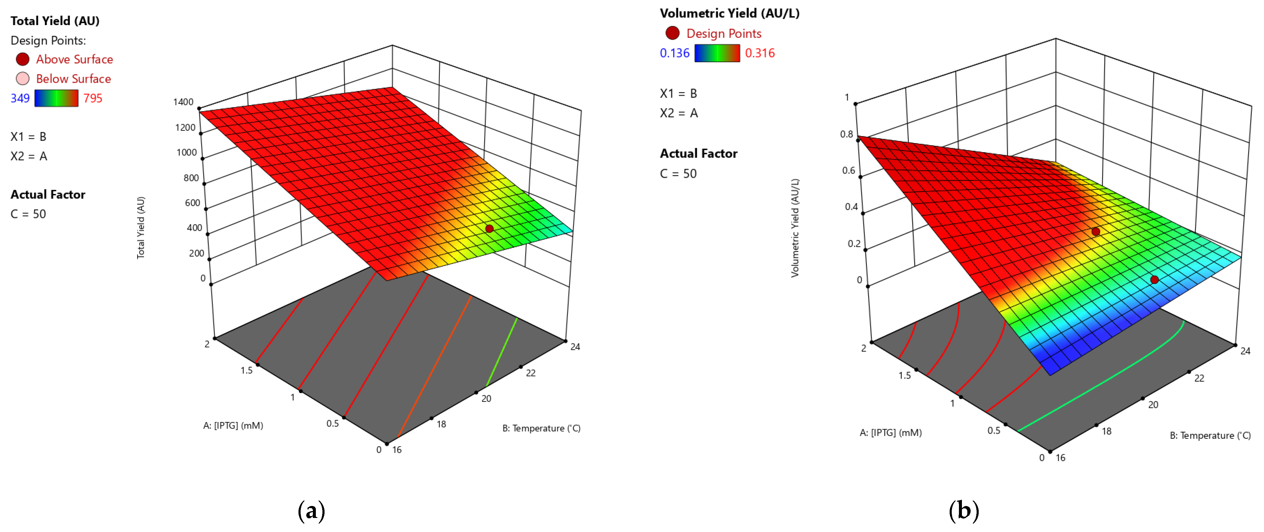
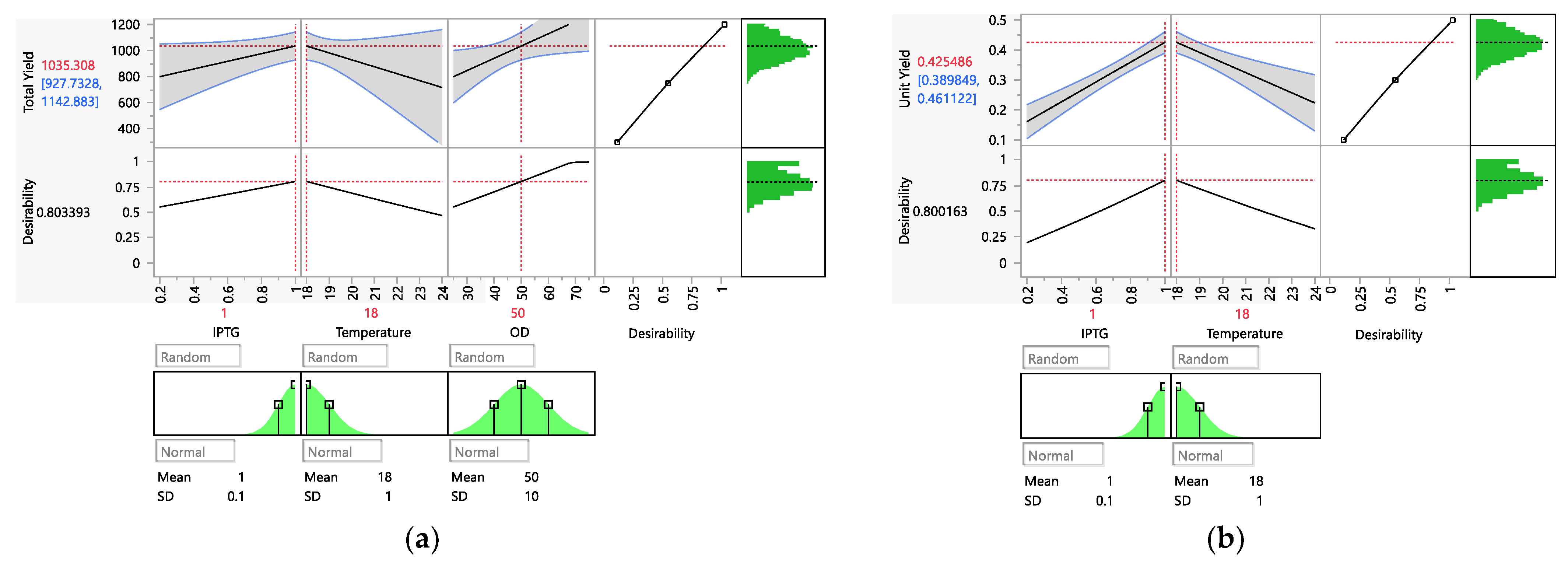
3.2. Optimization and Verification

On the basis of the analysis with the first eight data points, we found that there were two optimization attempts. The verifications are described as follows. In the first, condition 1, the temperature was 18 °C, and the inducer concentration was 1 mM. In the second, condition 2, the temperature was 17 °C, and the inducer concentration was 2 mM. Condition 1 was executed as runs 9, 10, and 11. The quality data confirmed that these conditions worked (Figure 2).

On the basis of the preliminary data, we found that condition 2 returned a higher quantity than condition 1 on the lab scale (a smaller fermenter). Then, both were examined in a CMO plant with a larger fermenter. Both conditions yielded better total product quantities, with 25% increases over run 5 (Table 1). However, the total yield of condition 2 was similar to that of condition 1 in the CMO fermenter. In summary, condition 2 returned a higher yield than condition 1 in a smaller fermenter but returned a similar quantity in a large fermenter.

The results may indicate differences between large and smaller fermenters (i.e., the scale-up parameters might not be suitable in this condition). In addition, the temperature of around 17 °C was a few degrees above the limit of the cold-water system, and therefore the process took more time. In the end, condition 2 was not used because of the higher cost of the inducer and longer time before induction (lower temperature and the limit of the system).

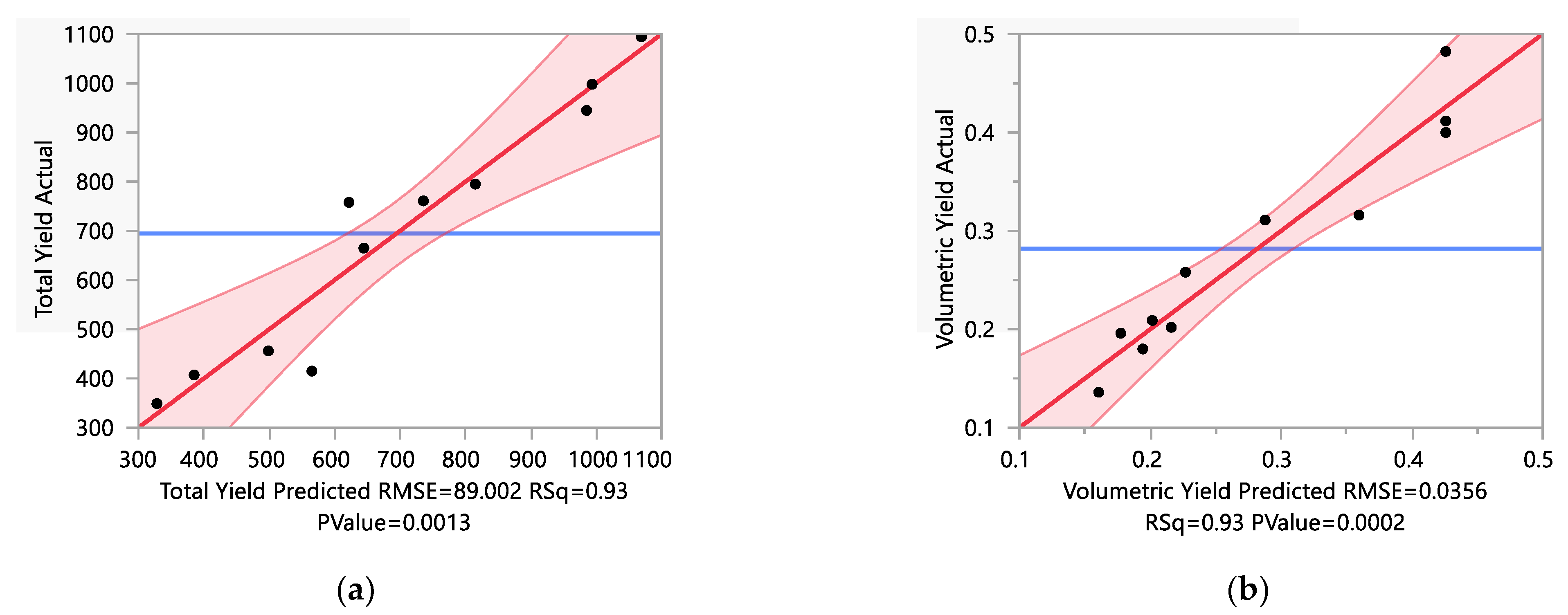
3.3. Final Set of Data and the Characterization of the Model

On the basis of the full data set of 11 runs, we built both of the models. The ANOVA analyses indicated that the total yield model had a low p-value of 0.0013. The RMSE was 89, average was 695, and C.V.% was 12.8. The R² was 0.93, and the adjusted R² was 0.88. The analyses indicated that the total yield had a significant variable of B × C = temperature × OD at p = 0.034 (

Table 2. Regression analysis of the model of the total yield model.

Analysis of Variance
Source	DF	Sum of Squares	Mean Squares	F Ratio
Model	4	623,649.62	155,912	19.6824
Error	6	47,528.51	7921
C. total	10	671,178.14
Parameter Estimates
Term	Estimate	Std Error	t Ratio	Prob > |t|
Intercept	758.4354	64.0169	11.85	<0.0001
IPTG (0.2,1)	113.7417	46.8964	2.43	0.0515
Temperature (18,24)	−129.9934	95.2465	−1.36	0.2213
OD (25,75)	11.5113	100.2911	0.11	0.9124
Temperature*OD	−198.0394	72.6126	−2.73	0.0343 *

* Variable identified as having a significant effect on response (p < 0.05).

). The coded (normalized) equation of the volumetric yield is shown in Equation (2), where A is [IPTG], B is temperature, and C is OD.

$$Total Yield=758.44+113.74\times A – 129.99\times B+11.51\times C – 198.04\times B C$$

(2)

The volumetric yield model returned a low p-value of 0.0002. The RMSE was 0.036, average was 0.282, and C.V.% was 12.6. The R² was 0.93, and the adjusted R² was 0.90. The analyses indicated that the volumetric yield had significant variables of A = [IPTG] at p = 0.003, B = temperature at p = 0.017, and A × B at p = 0.013 (

Table 3. Regression analysis of model of the volumetric yield model.

Analysis of Variance
Source	DF	Sum of Squares	Mean Squares	F Ratio
Model	3	0.11546754	0.038489	30.3715 &
Error	7	0.00887095	0.001267
C. total	10	0.12433849
Lack of Fit
Lack of fit	5	0.00489903	0.00098	0.4934
Pure error	2	0.00397192	0.001986
Total error	7	0.00887095
Parameter Estimates
Term	Estimate	Std Error	t Ratio	Prob > |t|
Intercept	0.2510369	0.012421	20.21	<0.0001
IPTG (0.2,1)	0.0736129	0.016402	4.49	0.0028 *
Temperature (18,24)	−0.042237	0.013629	−3.1	0.0173 *
IPTG * Temperature	−0.059079	0.017984	−3.29	0.0134 *

* Variable identified as having a significant effect on response (p < 0.05); ^&: p = 0.0002.

). The coded (normalized) equation of the volumetric yield is shown in Equation (3), where A is [IPTG] and B is temperature.

$$Volumetric Yield=0.251+0.074\times A – 0.042\times B – 0.059\times A\times B$$

(3)

Because the highest total yield and the volumetric yield were achieved in runs 9, 10, and 11, then using the Point Prediction function in the “Post Analysis” directory, we were able to predict the total yield to be on average 1002 ± 89 (885 to 1120, at 95% C.I., Figure 2a). Similarly, the volumetric yield was predicted to be 0.426 ± 0.036 (0.382 to 0.470 at 95% C.I., Figure 2b).

3.4. Final Set of Data Executed by JMP

On the basis of the full dataset of 11 runs, we also built both the total yield and volumetric yield models with JMP software. After similar procedures, the analyses indicated that both JMP and Design Expert software returned the same final total yield and volumetric yield models. The ANOVA analyses of the total yield are listed in Table 2, and those of the volumetric yield are listed in Table 3. The coded formula for total yield was the same as Equation (2). The coded formula for volumetric yield was the same as Equation (3). The plot of actual versus predicted values is shown in Figure 3.

The highest total yields and volumetric yields were those from runs 9, 10, and 11. Thus, the optimization focused on condition 1, with an inducer concentration of 1 mM and a temperature of 18 °C. The average of the simulations of the total yield was 1035.3 (927.7 to 1142.9). The average of the simulations of the volumetric yield was 0.425 (0.390 to 0.461). Data and distribution are presented in Figure 4.

4. Discussion

Software comparison: This study was analyzed in Design Expert and in JMP. Both programs returned the same models. The differences were in the optimization in the final stage. In Design Expert, a single average with a standard deviation was calculated. In JMP, we set the conditions such that the S.D. of inducer concentration, induction temperature, and induction OD were 1.0 ± 0.1 mM, 18 ± 1 °C, and 50 ± 10, and the additional distribution can be seen in Figure 4. We found these two kinds of software to be similar to the point of equivalence on the basis of this study.

After the models were built on the basis of eight data points, the Design Expert simulations indicated that, for an inducer concentration of 1 mM, induction temperature of 18 °C, and induction OD of 50, the predicted total yield would be 998 ± 110 and the predicted volumetric yield would be 0.40 ± 0.03. The later runs validated the predictions.

In this study, quadratic terms were forced in both software programs. None of the attempts returned significant results, and the ANOVA results were no better than those of these simpler models. Thus, the models were not included.

The final conditions for this drug were found to be 1.0 mM, 18 °C, and 50 induction OD. The expected total yield was simulated to be around 1020, and the volumetric yield, around 0.43. According to experience, the operation space of the inducer concentration was 1.0 ± 0.1 mM, the induction temperature was 18 ± 1 °C, and induction OD was 50 ± 10 (Figure 4). Studies including simulations may serve as supporting data for the determination of the (putative) critical process parameters and development of the fermentation process.

In the downstream process, after three purification steps, the lot-release specification of the final drug substance was around 98 ± 1 (%) in purity. After the first step of purification, the purity was low, with very large uncertainty. On the basis of the preliminary results of the scaling-up batches (data not shown), we found that the purity with a fixed condition after the first column was around 40% to 50%. Thus, the contribution of the fermentation process parameters to the quality of the product seems difficult to detect. Models will suffer from noise. After three steps of purification, the contributions were minimized. Thus, the quality attributes were assumed not to be correlated to the current three process parameters in the fermentation stage.

Provided that more data are analyzed, we can then know whether the simplest models can be applied to other systems. In addition, we hope that the above strategy or models can be applied to other recombinant protein systems.

5. Conclusions

This case study shows that linear regression models built on OFAT data can help researchers easily achieve optimization. From the addition of a few points, the volumetric yield model gained low p-values of 0.0002, with only main effects and primary interaction terms. The variables all significantly contributed to the model. The analysis can serve as supporting data for the determination of the operating space of the process parameters in future drug applications.

References

1. ICH. Pharmaceutical Development Q8(R2). Step 4 Version, August 2009. Available online: https://database.ich.org/sites/default/files/Q8_R2_Guideline.pdf (accessed on 26 November 2021).
2. U.S. Dood & Drug Administration. What Are the Points to Consider for the Role of Models in Quality by Design (qbd). Available online: https://www.fda.gov/regulatory-information/search-fda-guidance-documents/q8-q9-q10-questions-and-answers-appendix-qas-training-sessions-q8-q9-q10-points-consider#V._What_are_the_QBD_ (accessed on 26 November 2021).
3. U.S. Dood & Drug Administration. Quality by Design—Fda Lessons Learned and Challenges for International Harmonization. Available online: https://www.fda.gov/media/85369/download (accessed on 25 November 2021).
4. Tang, Y.; U.S. Dood & Drug Administration. Quality by Design Approaches to Analytical Methods—Fda Perspective. Available online: https://www.fda.gov/media/84046/download (accessed on 25 November 2021).
5. Lebrazi, S.; Niehaus, K.; Bednarz, H.; Fadil, M.; Chraibi, M.; Fikri-Benbrahim, K. Screening and optimization of indole-3-acetic acid production and phosphate solubilization by rhizobacterial strains isolated from acacia cyanophylla root nodules and their effects on its plant growth. J. Genet. Eng. Biotechnol. 2020, 18, 71. [Google Scholar] [CrossRef] [PubMed]
6. Lebrazi, S.; Fadil, M.; Chraibi, M.; Fikri-Benbrahim, K. Screening and optimization of indole-3-acetic acid production by rhizobium sp. Strain using response surface methodology. J. Genet. Eng. Biotechnol. 2020, 18, 21. [Google Scholar] [CrossRef] [PubMed]
7. Giovanni, M. Response surface methodology and product optimization. Food Technol. 1983, 37, 5. [Google Scholar]
8. Chidambaram, N. Cder Regulatory Applications—Investigational New Drug and New Drug Applications. Available online: https://www.fda.gov/media/91746/download (accessed on 26 November 2021).
9. U.S. Dood & Drug Administration. Pat—A-Framework-for-Innovative-Pharmaceutical-Development-Manufacturing-And-QUALITY-assurance. Available online: https://www.fda.gov/media/71012/download (accessed on 26 November 2021).
10. Kelley, B. Industrialization of mab production technology: The bioprocessing industry at a crossroads. Mabs 2009, 1, 443–452. [Google Scholar] [CrossRef] [PubMed] [Green Version]
11. Appel, R.D.; Bairoch, A.; Hochstrasser, D.F. A new generation of information retrieval tools for biologists: The example of the expasy www server. Trends Biochem. Sci. 1994, 19, 258–260. [Google Scholar] [CrossRef]
12. Available online: Http://au.Expasy.Org/tools/protparam-doc.Html, http://au.Expasy.Org/cgi-bin/protparam (accessed on 26 November 2021).
13. Kenneth, P.; Burnham, D.R.A. Multimodel inference: Understanding aic and bic in model selection. Sociol. Methods Res. 2004, 33, 261–304. [Google Scholar]
Figure 1. Numerical optimization presentation of the two models. (a) Total yield model: The design points are depicted in dark red if the corresponding total yield (actual) values were above those of the model (predicted value is the plane) and in pink if the actual value was lower than the predicted value. The predicted values from the model are color-coded in red for high and close to 795 or above, and blue for low. (b) Volumetric yield model: The design points are depicted in dark red if the corresponding total yield (actual) values were above those of the model (predicted value) and in pink if the actual value was lower than the predicted value. The predicted values from the model are color-coded in red for high and close to 0.316 or above and in blue for low. OD values were set as 50.
Processes 10 00237 g001
Figure 2. Numerical optimization presentation of the two models. (a) Total yield model: The design points are depicted in dark red if the corresponding total yield (actual) values were above those of the model (predicted value is the plane) and depicted in pink if the actual value was lower than the predicted value. The predicted values from the model are color-coded as red for high and close to 1094 or above and blue for low. (b) Volumetric yield model: The design points are depicted in dark red if the corresponding total yield (actual) values were above those of the model (predicted value) and depicted in pink if the actual value was lower than the predicted value. The predicted values from the model are color-coded as red for high and close to 0.482 or above and blue for low. OD values were set as 50.
Processes 10 00237 g002
Figure 3. Prediction plot vs. actual plot for (a) total yield model: the uncertainties are shaded red and the R2 = 0.93; (b) volumetric yield model: the uncertainties are shaded red and R2 = 0.93. The statistics can be found in Table 2 and Table 3.
Processes 10 00237 g003
Figure 4. Prediction profiler for process optimization and simulation studies with Monte Carlo simulations of 10,000 runs with different data distribution types (shaded regions) and S.D. The inducer concentration, induction temperature, and induction OD were set at 1.0 ± 0.1 mM, 18 ± 1 °C, and 50 ± 10, respectively. (a) Total yield model; (b) volumetric yield model.
Processes 10 00237 g004