Abstract
In industrial practice, excessive alarms and high alarm rates are mostly generated from unreasonable settings to variable alarm thresholds, which have become the significant causes of impact on operation stability and plant safety. A correlation degree and clustering analysis-based approach was presented to optimize the variable alarm thresholds in this paper. The correlation degrees of variables are first obtained by analyzing correlation relationships among them. Second, the variables are grouped according to the gray correlation coefficients and clustering analysis, given the weight for fault alarm rate (FAR) in each group. An objective function about the FAR, missed alarm rate (MAR), and the maximum acceptable FAR and MAR is then established with variable weight. Eventually, based on an optimization algorithm, the objective function can be optimized for obtaining the optimal alarm threshold. Cases study of the Tennessee Eastman (TE) industrial simulation process and an actual industrial ethylene production process, in comparison to the initial situation, show that the method can effectively reduce FAR according to correlation degrees among variables in the system, and decrease the number of alarms with reduction rates of 40.5% and 35.3%, respectively.
1. Introduction
With the complexity and refinement of the process of industrial production, the production process is more and more inseparable from real-time monitoring of the system. An alarm management system, as an indispensable part in the safety operation of industrial production, has been paid more and more attention by all walks of life. In industrial practice, cases with more false alarms, a higher false alarm rate (FAR) and a missed alarm rate (MAR) always arise in processes [1], which are mainly caused through the unreasonable threshold settings for variables and ineffective management for alarm systems. Based on the studies from EEMUA, the range of alarm numbers that an operator could effectively handle for one alarm is from every 5 min to 10 min [2].
Regarding the methods of alarm optimization, academia has given many methods, each of which plays a certain role in its corresponding system to a greater or lesser extent. There are many kinds of alarm optimization methods, and classification methods are inconclusive. Generally speaking, they can be divided into univariate methods and multivariate methods, threshold optimization methods and algorithm optimization methods, off-line methods and dynamic methods, etc.
For determining the process variable threshold, academia has studied many optimization methods. For instance, in terms of FAR and MAR, an approach for estimating the threshold was proposed on account of an adaptive fuzzy-neural network and genetic learning algorithm [3]. As the threshold can be determined by the deadband, a method with the objective function about FAR and MAR, and the relation between the optimal threshold and deadband to estimate the threshold, was presented [4]. Combining FAR and MAR with a correlation coefficient, an off-line method for optimizing thresholds was given to reduce alarms for multi-variables based on time delay [5]. For improving the robustness classification performance in the system with regard to separation threshold selection, different intelligent pattern classifiers were used to mine industrial batch dryer data to determine thresholds [6]. In addition, there also have many methods in setting thresholds in early warning and damage systems [7,8], alarms reduction [9], systems monitoring [10,11], and performance optimization [6,12].
Over the past five years, based on intelligent algorithms, some similar methods have been improved. For instance, to remove chattering alarms, a univariate method was presented for addressing the reduction of alarms with median filters [13]. Taking the missed alarms and false alarms into account, an off-line univariate approach for determining alarm threshold in debris flow forecasting was presented, with the lowest missed-alarm and false-alarm probabilities [14]. By optimizing positioning accuracy, the pulse-width multiplexing Φ-OTDR and multisensor information fusion algorithm were utilized to reduce the nuisance alarm rate [15]. For target tracking in a chaotic environment, a mul-tivariate approach was proposed to optimize the joint threshold and power allocation strategy with a two-variable nonconvex optimization problem for the cognitive radar network, containing the detection stage and transmitting stage [16]. Based on the test observations, an off-line simple and robust approach was proposed to determine the detection thresholds for detecting defluidization in the early stage [17]. Some approaches about optimal alarm identification [18], design and evaluation analysis for an alarm system [19,20,21,22,23], management framework [24], alarm threshold [25], and an overview of industrial alarm systems [26] also have appeared. Variables in most of the above approaches have not been clustered with optimized thresholds, which could be suitable for analyzing interlinks among similar variables. Therefore, Zhang et al. presented an off-line multivariate method based on ROC curve and sensitivity, considering the sensitivity relationship and clustering analysis among variables, to optimize the alarm threshold [27]. A multivariate alarm clustering method was proposed that takes advantage of the information contained in the alarm logs themselves, of which the clustering analysis for process alarms was achieved through word embedding [28]. Analyzing alarm data, Lucke et al. presented an on-line method that conducted a practical application for alarm flood classification based on a set of historical alarm floods [29]. In the process, for high-dimension variables, the number of alarms needing addressing increases significantly when the number of measurable variables increases. False alarms caused by redundant disturbances will disturb operators, leading to alarms having more significance on the system being missed as a consequence. Thus, clustering variables into groups is necessary for alarm optimization.
Most of the above alarm optimization methods are based on the off-line system optimization, and the results obtained in the corresponding systems are also obvious, large or small, effectively optimizing the production process and reducing losses. Thus, to promptly detect the chattering alarms and effectively reduce the number of chattering alarms, an on-line method was given to detect alarms in a timely manner [30]. As for the HVAC systems, Chakraborty et al. put forward a novel dynamic threshold method with a data-driven model using extreme gradient boosting (XGBoost), which mainly utilized early fault detection [31]. The static and dynamical performance analyses were used to update evidence in designing the industrial alarm system to reduce unnecessary alarms [32]. There are also some corresponding approaches for optimization, such as alarm management strategy [33], alarming mechanism [34], and threshold setting [35], which have promoted the development of dynamic methods to a certain extent.
However, as the current industrial production processes change irregularly, the preceding production process and the following process cannot be consistent all the time, such as the changes caused by different conditions or an abnormal process. In view of the problem, a new alarm threshold optimization method is proposed, which uses the correlation degrees among the variables and clustering analysis. Herein, this paper mainly has four significant contributions. (1) It considers the gray correlation degree analysis. Variables with similar influence on the system can be found out through correlation analysis. (2) It could carry on the group sorting according to the intrinsic clustering analysis. (3) It reduces FAR and also has a significant inhibitory effect on MAR (significantly reduced invalid alarms). (4) It can be used as a reference for real-time online optimization. When connecting the current programs to the computer interface in on-line systems, it could meet the requirements of the fast-changing production processes through setting an update period and data, which would consider the alarm rates. In addition, this method could help operators reduce operation load, make more efficient repair measures in a timely manner, and reduce the losses.
2. Optimum Design Outline
2.1. Alarm Efficiency Index
At present, an alarm system is important for safety, which generally utilizes FAR and MAR as efficiency indices to measure the accuracy of detecting operation conditions [36]. Based on the operation conditions, industrial processes usually contain normal and abnormal situations, which generally use the FAR and MAR to represent the probability directly for a variable when its measured values go beyond the threshold in normal operations, and within the threshold in abnormal operations in an alarm system [37].
The FAR and MAR can be obtained as follows:
Initially, for a variable x, within a period of time, two groups of data under normal and abnormal situations are obtained. Where a group of data are collected as the normal data when the process runs normally and steadily, another set of data are collected as the abnormal data when the process deviates from normal operation state obviously, which contains added disturbance or failure.
Later, for a variable x, the probability density functions f(x) and g(x) under the two situations, respectively, are obtained by fitting the corresponding data, which can be shown in Figure 1, where xT denotes as the alarm threshold. For a certain parameter of the system, xT indicates that the parameter has a well running state under the current threshold. When it exceeds or falls below the current threshold, the process may generate redundant false alarms or missed alarms. Here, false alarms will be activated when normal process variable values (the blue line) falls below xT, and missed alarms will be activated when the abnormal process variable values (red dotted line) exceed xT.
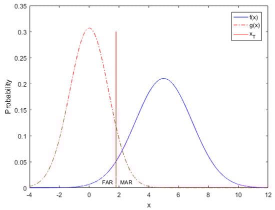
Figure 1.
Process probability density curves of x.
Finally, given the , based on Figure 1 and the Equations (1) and (2) [5,36], the FAR and MAR can be obtained.
The following work in this paper can be conducted when the functions (f(x) and g(x)) for a variable can be fitted which was irrelevant to the distribution.
2.2. Alarm Clustering Analysis
Based on the alarm clustering algorithm, variables can be clustered into groups.
- Correlation degree analysis
A measure of the degree of correlation between two factors in a system that varies from time to time or from object to object is called the correlation degree [38]. In a system process, if the trend of change of the two factors is consistent, that is, the degree of synchronous change is high, then the degree of correlation is high. Conversely, it is lower. Thus, the gray correlation analysis method is a method to measure the correlation degree among factors according to the degree of similarity or difference of development trend among factors, that is, “gray correlation degree”.
Specific calculation steps for correlation analysis:
- (1)
- Determine the reference sequence and comparison sequence. The data sequence that reflects the behavior characteristics of a system is called a reference sequence and the data sequence composed of factors that affect the behavior of a system is called a comparison sequence;
- (2)
- Conduct dimensionless treatment for the reference sequence and comparison sequence.
Due to the different physical meanings of each factor in the system, the dimensionality of the data may not be the same, which is not convenient for comparison, or it is difficult to get the correct conclusion when comparing. Therefore, in the analysis of gray relational degree, dimensionless data processing should be generally required.
- (3)
- Determine the reference sequence and comparison sequence of the gray correlation coefficient ξ(Xi).
The correlation degree is essentially the difference in geometry among curves. So, the difference among curves can be used as a measure of the correlation degree. For a reference sequence , there are several comparison sequences X1, X2, …, Xm, the correlation coefficient ξi(k) of each reference sequence and comparison sequence each time is deduced by the following formula:
where, P is the distinguish coefficient, the value range of which is generally between 0–1, with 0.5 as the common value; represents the absolute difference between the sequences Xi and X0 at point k; l = 1, 2, …, n, is the minimum difference of the first level, which represents the minimum difference between sequences Xj(l) and X0(l) at each point; is the minimum difference of the second level, which represents the minimum difference in all sequences based on the minimum difference found in each sequence; is the maximum difference of the first level, which represents the maximum difference between sequences Xj(l) and X0(l) at each point; is the maximum difference of the second level, which represents the maximum difference in all sequences based on the maximum difference found in each sequence.
In order to avoid the resulting deviation caused by variable units and other factors, it is necessary to conduct standardized processing on variable data.
- (4)
- Calculate the correlation degree
As the correlation coefficient denotes the value of correlation degree between the comparison sequence and the reference sequence at each time, it has more than one value, which could lead the information to be too scattered to facilitate the overall comparison. Therefore, it is necessary to concentrate the correlation coefficient of each moment into a value, that is, to find its average value, as the value expression of the correlation degree between the comparison sequence and the reference sequence.
Correlation degree ri represents the gray correlation degree of comparison sequence Xi to reference sequence X0, also called sequence correlation degree, average correlation degree, and line correlation degree, the formula of which is shown as follows:
The closer the value of ri is to 1, the better the correlation is.
- 2.
- Clustering analysisSpecific clustering steps:
- (1)
- Calculate the gray correlation coefficients between every two variables, then sum the distances;
- (2)
- Calculate the correlation degree standard deviations of the above sums, utilizing wd to denote the deviation result;
- (3)
- Based on the relationship between wd (the value obtained by 0–1 normalization for the summation of the correlation coefficients of one variable to all other variables) and Cg (global correlation degree level), and the relation of Pearson correlation coefficients and correlation levels [39], variables are clustered into groups, listed in Table 1. Then, the variable weight of a variable in one group can be calculated through the data of variables in the group.
 Table 1. Relationship between the values of wd and Cg.
- 3.
- Variable weight calculation
The variable weight of a variable in one group can be determined through the mean square error method with specific steps, as below:
- (1)
- Data normalizationwhere, denotes the initial data of the jth variable in group i.
- (2)
- Mean value
- (3)
- Mean square error
- (4)
- Variable weight
Herein, two efficiency indices are introduced totally, FAR and MAR. Compared with MAR, the correlation degree mainly reflects on FAR, which has a significant effect on the system. Therefore, the weight wij is given for FAR. Meanwhile, MAR/RMAR is used in case of overlarge MAR, where RMAR denotes the maximum acceptable MAR, values of which generally less than the engineering required error (0.05) with 0.01, recommended by [2].
2.3. Threshold Optimization
The optimization objective function, shown as Equation (9), is established according to the alarm information under normal and abnormal situations, which is solved by the numerical optimization method from the point of view of minimizing.
where, denotes the maximum acceptable FAR, the value of which generally less than the engineering required error (0.05) with 0.01, recommended by [2].
Figure 2 depicts the flow chart of a quadratic interpolation optimization algorithm with the basic thought shown as: for F(x) = Min φ(x) (x∈R1), the φ(x) can be fitted by y(x), which consists of some dots. Then, the extreme point μ of y(x) is an estimate value of x*.
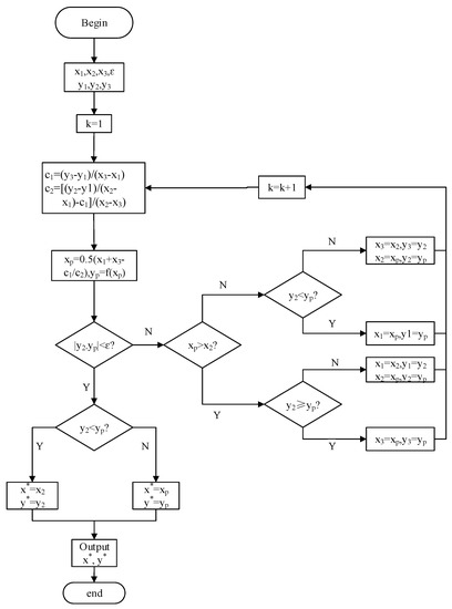
Figure 2.
Flow diagram of quadratic interpolation optimization algorithm.
A threshold optimization algorithm is implemented as follows:
- (1)
- Give the initial interval [x1,x3], three points (x1, y1), (x2, y2), (x3, y3), and convergence precision ε, where, x1 < x2 < x3, ε > 0;
- (2)
- Calculate c1, c2 (where, c1 = (y3 − y1)/(x3 − x1), c2 = [(y2 − y1)/(x2 − x1) − c1]/(x2 − x3)), and xp = 0.5(x1 + x3 − c1/c2), yp = f(xp);
- (3)
- If |y2 − yp| ≥ ε, then go step (4), otherwise, go step (9);
- (4)
- If xp > x2, then go step (5), otherwise, go step (7);
- (5)
- If y2 ≥ yp, then x3 = xp, y3 = yp, return to step (2) otherwise, go step (6);
- (6)
- Let x1 = x2, y1 = y2, x2 = xp, y2 = yp, return to step (2);
- (7)
- If y2 < yp, then x1 = xp, y1 = yp, return to step (2) otherwise, go step (8);
- (8)
- Let x3 = x2, y3 = y2, x2 = xp, y2 = yp, return to step (2);
- (9)
- If y2 < yp, then x* = x2, y* = y2, otherwise, go step (10);
- (10)
- x* = xp, y* = yp;
- (11)
- Output x* = xp, f* = f (x*).
2.4. Optimization Process Description
Figure 3 gives the optimization algorithm, the specific explanations of which are shown as follows:
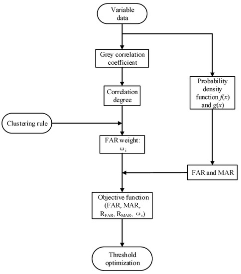
Figure 3.
Flow chart of alarm threshold optimization process.
To begin with, the correlation degrees of variables are obtained by analyzing correlation relationships among them. Subsequently, the variables are grouped according to the gray correlation coefficients and clustering analysis, given the weight ωi for FAR in each group. An objective function about the FAR, MAR, RFAR, RMAR, and ωi is then established with variable weight. Eventually, based on the optimization algorithm, the objective function is optimized for obtaining the optimal alarm threshold.
3. Theory Study—Tennessee Eastman (TE) Simulation Process
3.1. Process Description
TE process was put forward by J. J. Downs and E. F. Vogel. It can be used as a data source, which is commonly utilized for comparing various methods, such as control optimization. Therefore, this work uses the TE simulation process as a case.
Figure 4 shows the flow diagram for a TE process, which contains five major operating units: reactor, condenser, compressor, separator, and stripper. The TE process consists of 15 known failures and 5 unknown failures. Meanwhile, it also consists of 12 operational variables and 41 measured variables. Table 2 lists the selected 10 measured variables for researching the applicability analysis of the method. To verify the accuracy of the results, the same sampling environment (the faults were after 8 simulation hours introduced) should be necessary, sampling interval of which is ΔT = 3 min by considering the time constants of the process in a closed loop [40,41], as the process under the sampling time can be considered reaches a relatively steady running state, which could reflect the running state with a long period of time, to some extent. Meanwhile, 960 groups of data under a normal condition and 500 groups of data under an abnormal condition with failure 6 are collected.
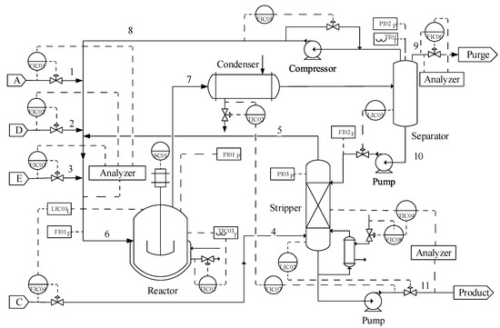
Figure 4.
Flow chart of TE process.
Table 2.
Ten measured variables in TE process.
3.2. Cluster Variables and Calculate Weights
- (1)
- Variable clustering
The selected ten variables can be regarded as 10 vectors with 960 dimensions, containing 960 observations of normal data. Table 3 lists the correlation degree of these ten variables.
Table 3.
Correlation degree of ten variables.
Calculating the sum (dT) of the correlation degree between one variable and all other variables is necessary for treating ten variables as a whole. Table 4 lists the sums and the normalized result (wd).
Table 4.
Sums of the correlation degree and normalized result of ten variables.
Based on the normalization result and criterions given in Table 1, the original ten variables are clustered into four groups. Variables V1 and V2 constitute the first group, variable V3 constitutes the second group, variable V6 constitutes the third group and the rest belong to the last group.
- (2)
- Variable weight
Table 5 lists the weights for variables in four groups.
Table 5.
Variable weights.
For the FAR and MAR, the impact on the system caused by the correlation degree of variables commonly reflect on FAR more directly than MAR, therefore, giving the correlation weight to FAR.
3.3. Optimization Solution
Steps of the optimization solution are listed as below, using the first variable V1 as an example.
First, the probability density function Equations (10) and (11) of V1 in the normal and abnormal cases are fitted with 960 observations of normal data and 500 observations of abnormal data, respectively. Figure 5 shows the corresponding probability density curves.
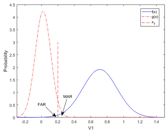
Figure 5.
Process probability density curves of V1.
Second, the objective function is obtained as Equation (12), the parameters of which, including weight w1 = 0.521, Equations (1) and (2), RFAR = RMAR = 0.01, are input into function Equation (9).
Eventually, the objective function is optimized as Figure 6, with optimum xT = 0.22, F(xT) = 6.5098, FAR = 0.00654, MAR = 0.06710. The thresholds of other variables are optimized similarly.
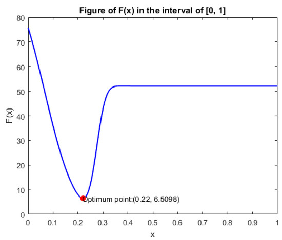
Figure 6.
Optimization result of V1.
Additionally, to verify the effectiveness of this method, some other methods should be utilized for comparison, such as the deadband [42], alarm delay [36], and moving average filter (MAF) with original reference value [27]. The summarized results listed in Table 6.
Table 6.
Optimized results for ten variables.
To verify the effectiveness of the method, an abnormal data set of fault 8 is added. Table 6 lists the results under the two failures (failure 6: f6, failure 8: f8).
3.4. Results and Analysis
Shown in Figure 7, the FAR calculated by the proposed method has an effective reduction in cases with initial thresholds, and the MAR of which under control simultaneously.
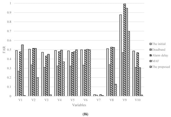
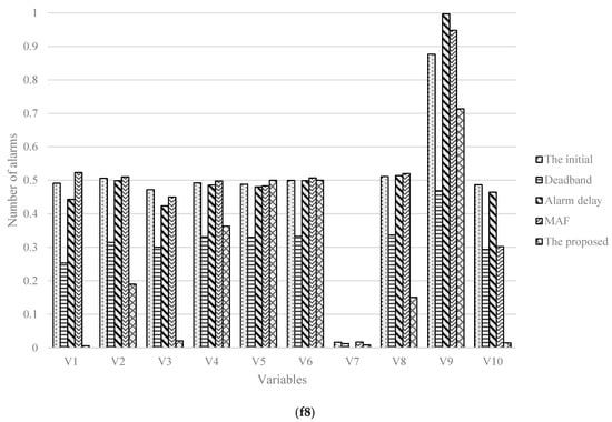
Figure 7.
Histograms of FARs in five cases with two failures (f6,f8).
In Figure 8, the numbers of variable alarms in total under 5 cases under the case with failure 6 (8) are 3532, 3414, 2916, 2928, 1733 (3532, 3417, 2968, 2992, 1744), respectively. Compared with the other four methods, the alarm reduction rates calculated by the presented method are 50.9%, 49.2%, 40.5%, and 40.8% (50.6%, 48.9%, 41.2%, and 41.7%), respectively. From which, it reflects the method could have some impact on the alarm threshold optimization, bring a lower FAR and fewer alarms.
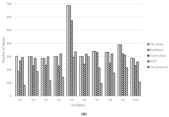
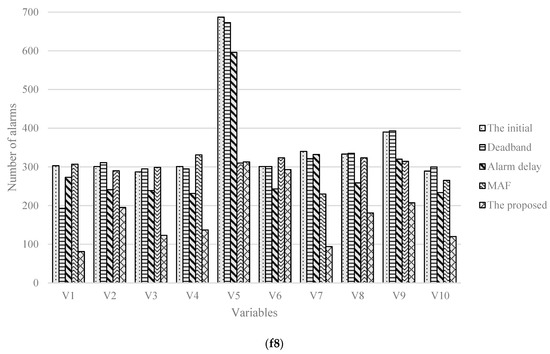
Figure 8.
Histograms of number of alarms in five cases with two failures (f6,f8).
4. Real Industrial Verification—Industrial Ethylene Production Process
4.1. Process Description
To verify the effectiveness of the method in actual industry, an industrial ethylene production process was selected as an actual case, the process of which generally consists of four major processes: cracking, compression, quenching, and separation.
Figure 9 shows the flow chart of the ethylene production process, the separation section of which contains the most of research object. Due to the large number of variables in this process, in order to avoid the influence of blind selection on the results, we try to objectively select variables with correlation relationships among them not easy to judge and which have significant impact on the yield and quality of ethylene through empirical knowledge and analysis. Therefore, ten variables are selected to represent the process, which are listed in Table 7. For this process, the time-lag effect under start-up or shut-down cases is great. Therefore, the data under the steady state are selected as normal data and the data under the state with disturbances are then chosen as abnormal data for study, respectively, are selected for study. In total, 1000 observations of data for 10 variables are extracted with a sampling interval of 1 min, containing 500 observations of normal data and 500 observations of abnormal data with the feed flow of cracking furnace increases by 10%.
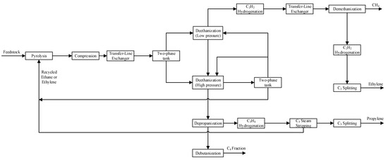
Figure 9.
Flow chart of ethylene production process.
Table 7.
Ten measured variables in ethylene production process.
4.2. Cluster Variables and Calculate Weights
- (1)
- Variable clustering
The selected ten variables can be regarded as 10 vectors with 500 dimensions, containing 500 observations of normal data. Table 8 lists the correlation degree of these 10 variables.
Table 8.
Correlation degree of 10 variables.
Calculating the sum (dT) of the correlation degree between one variable and all other variables is necessary for treating ten variables as a whole. Table 9 lists the sums and the normalized result (wd).
Table 9.
Sums of the correlation degree and normalized result of ten variables.
Based on the normalization result and criterions given in Table 1, the original ten variables are clustered into four groups. Variables V1, V4, and V7 constitute the first group, variables V2 and V8 constitute the second group, variable V10 constitutes the third group and the rest belong to the last group.
- (2)
- Variable weight
Table 10 lists the weights for variables in four groups.
Table 10.
Variable weights.
4.3. Optimization Solution
Steps of the optimization solution are listed as below, using the first variable V1 as an example.
First, the probability density functions Equations (13) and (14) of V1 in normal and abnormal cases are fitted with 500 observations of data, respectively. Figure 10 shows the corresponding probability density curves.
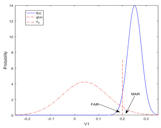
Figure 10.
Process probability density curves of V1.
Second, the objective function is obtained as Equation (15), parameters of which in-cluding weight w1 = 0.453, Equations (1) and (2), RFAR = RMAR = 0.01 are inputted into function Equation (9).
Eventually, the objective function is optimized as Figure 11, with optimum xT = 0.73, F(xT) = 6.5095, FAR = 0.00354, MAR = 0.0661. The thresholds of other variables are optimized similarly.
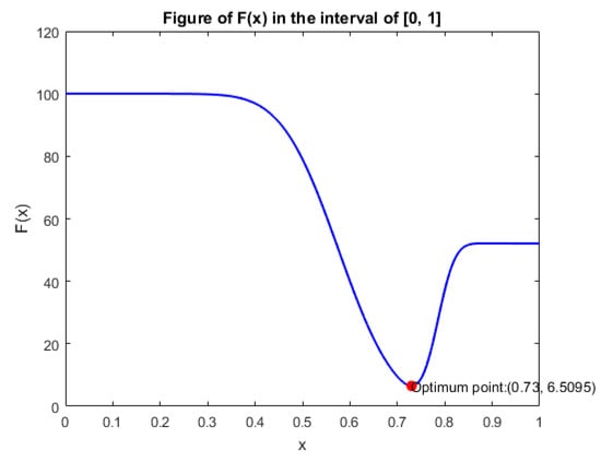
Figure 11.
Optimization result of V1.
To verify the effectiveness of the method, an abnormal data set of the feed flow of cracking furnace decreases by 10% and is added. Table 11 lists the results under the two cases (cracking furnace increases by 10%: c1, cracking furnace decreases by 10%: c2).
Table 11.
Optimized results for 10 variables.
4.4. Results and Analysis
Shown as the Figure 12, the FAR calculated by the proposed method has an effective reduction in cases with initial thresholds, and the MAR of which under control simultaneously.
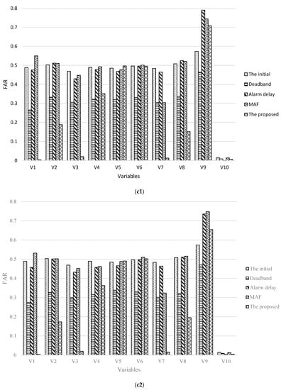
Figure 12.
Histograms of FARs in five cases with two cases (c1,c2).
In Figure 13, the numbers of variable alarms in total under 5 cases under the case of c1 (c2) are 2552, 2434, 2036, 2248, 1316 (2552, 2430, 2129, 2239, 1346), respectively. Compared with the other four methods, the alarm reduction rates calculated by the method are 48.4%, 45.9%, 35.3%, and 41.4% (47.2%, 44.6%, 36.8%, and 39.9%), respectively. From which, it reflects the method could have some impact on the alarm threshold optimization, bring a lower FAR and fewer alarms.
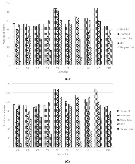
Figure 13.
Histograms of number of alarms in five cases with two cases (c1,c2).
5. Conclusions
In this work, correlation degree and clustering analysis based method is presented to achieve threshold optimization: the gray correlation coefficients of variables are first obtained by analyzing correlation degrees among them; the variables are grouped later according to the correlation degree and clustering analysis, given the weight ωij for FAR in each group; optimization algorithm is finally utilized to optimize objective function about FAR, MAR, RFAR, RMAR, and ωij to complete threshold optimization.
According to the analysis of case theory study with TE simulation process and actual industrial verification for industrial ethylene production process, the results manifest the presented approach can not only reduce FAR, have significant inhibitory effect on MAR, and decrease the number of alarms effectively in total, but could carry on the grouping sorting according to the intrinsic clustering analysis, which could help operators reduce operation load. Meanwhile, it will also leave operators more time to make more efficient repair measures timely and reduce losses through helping them to identify variables that have larger and more rapid impact on system, extend the deteriorative time for abnormity.
Author Contributions
Methodology, Z.W. and G.Z.; Writing—original draft preparation, G.Z.; Writing—review and editing, Z.W. and G.Z.; Supervision, Z.W. All authors have read and agreed to the published version of the manuscript.
Funding
Support for carrying out this work was provided by the National Key R&D Program of China (2018YFB1701103), International (Regional) Cooperation and Exchange Project (61720106008), and National Science Fund for Distinguished Young Scholars (61725301).
Institutional Review Board Statement
Not applicable.
Informed Consent Statement
Not applicable.
Conflicts of Interest
The authors declare no conflict of interest.
References
- Izadi, I.; Shah, S.L.; Shook, D.S.; Chen, T. An Introduction to Alarm Analysis and Design. IFAC Proc. Vol. 2009, 42, 645–650. [Google Scholar] [CrossRef] [Green Version]
- EEMUA. Alarm System: A Guide to Design, Management, and Procurement, 2nd ed.; The Engineering Equipment and Materials Users Association (EEMUA): London, UK, 2007. [Google Scholar]
- Mezache, A.; Slitani, F. A novel threshold optimization of ML-CFAR detector in Weibull clutter using fuzzy-neural networks. Signal Process. 2007, 87, 2100–2110. [Google Scholar] [CrossRef]
- Naghoosi, E.; Izadi, I.; Chen, T. A study on the relation between alarm deadbands and optimal alarm limits. In Proceedings of the American Control Conference, San Francisco, CA, USA, 29 June–1 July 2011. [Google Scholar]
- Han, L.; Gao, H.H.; Xu, Y.; Zhu, Q.X. Combining FAP, MAP and correlation analysis for multivariate alarm thresholds opti-mization in industrial process. J. Loss Prev. Process Ind. 2016, 40, 471–478. [Google Scholar] [CrossRef]
- Levente, L.S.; Konrad, H. Industrial batch dryer data mining using intelligent pattern classifiers: Neural network, neuro-fuzzy and Takagi–Sugeno fuzzy models. Chem. Eng. J. 2010, 157, 568–578. [Google Scholar]
- Burgess, L.P.; Herdman, T.H.; Berg, B.W.; Feaster, W.W.; Hebsur, S. Alarm limit settings for early warning systems to identify at-risk patients. J. Adv. Nurs. 2009, 65, 1844–1852. [Google Scholar] [CrossRef]
- Zhou, H.; Ni, Y.; Ko, J. Structural damage alarming using auto-associative neural network technique: Exploration of environment-tolerant capacity and setup of alarming threshold. Mech. Syst. Signal Process. 2011, 25, 1508–1526. [Google Scholar] [CrossRef]
- Chen, T. On reducing false alarms in multivariate statistical process control. Chem. Eng. Res. Des. 2010, 88, 430–436. [Google Scholar] [CrossRef] [Green Version]
- Jablonski, A.; Barszcz, T.; Bielecka, M.; Breuhaus, P. Modeling of probability distribution functions for automatic threshold calculation in condition monitoring systems. Measurement 2013, 46, 727–738. [Google Scholar] [CrossRef]
- Van Wynsberge, S.; Gilbert, A.; Guillemot, N.; Payri, C.; Andréfouët, S. Alert thresholds for monitoring environmental variables: A new approach applied to seagrass beds diversity in New Caledonia. Mar. Pollut. Bull. 2013, 77, 300–307. [Google Scholar] [CrossRef]
- Simşek, B.; İç, Y.T. Multi-response simulation optimization approach for the performance optimization of an Alarm Monitoring Center. Saf. Sci. 2014, 66, 61–74. [Google Scholar] [CrossRef]
- Sun, Y.; Tan, W.; Chen, T. A method to remove chattering alarms using median filters. ISA Trans. 2018, 73, 201–207. [Google Scholar] [CrossRef] [PubMed]
- Wu, M.-H.; Wang, J.P.; Chen, I.-C. Optimization approach for determining rainfall duration-intensity thresholds for debris flow forecasting. Bull. Eng. Geol. Environ. 2018, 78, 2495–2501. [Google Scholar] [CrossRef]
- Zhong, X.; Zhao, S.; Deng, H.; Gui, D.; Zhang, J.; Ma, M. Nuisance alarm rate reduction using pulse-width multiplexing Φ-OTDR with optimized positioning accuracy. Opt. Commun. 2020, 456, 124571. [Google Scholar] [CrossRef]
- Sun, H.; Li, M.; Zuo, L.; Cao, R. Joint threshold optimization and power allocation of cognitive radar network for target tracking in clutter. Signal Process. 2020, 172, 107566. [Google Scholar] [CrossRef]
- Jaber, S.; Pierre, S.; Jamal, C. A simple and robust approach for early detection of defluidization. Chem. Eng. J. 2017, 313, 144–156. [Google Scholar]
- Venkidasalapathy, J.A.; Mannan, M.S.; Kravaris, C. A quantitative approach for optimal alarm identification. J. Loss Prev. Process. Ind. 2018, 55, 213–222. [Google Scholar] [CrossRef]
- Aslansefat, K.; Gogani, M.B.; Kabir, S.; Shoorehdeli, M.A.; Yari, M. Performance evaluation and design for variable threshold alarm systems through semi-Markov process. ISA Trans. 2020, 97, 282–295. [Google Scholar] [CrossRef]
- Kaced, R.; Kouadri, A.; Baiche, K. Designing alarm system using modified generalized delay-timer. J. Loss Prev. Process. Ind. 2019, 61, 40–48. [Google Scholar] [CrossRef]
- Lucke, M.; Chioua, M.; Grimholt, C.; Hollender, M.; Thornhill, N.F. Integration of alarm design in fault detection and diagnosis through alarm-range normalization. Control. Eng. Pract. 2020, 98, 104388. [Google Scholar] [CrossRef]
- Taheri-Kalani, J.; Latif-Shabgahi, G.; Shooredeli, M.A. On the use of penalty approach for design and analysis of univariate alarm systems. J. Process. Control. 2018, 69, 103–113. [Google Scholar] [CrossRef]
- Wang, J.; Li, H.; Huang, J.; Su, C. A data similarity based analysis to consequential alarms of industrial processes. J. Loss Prev. Process. Ind. 2015, 35, 29–34. [Google Scholar] [CrossRef]
- Goel, P.; Pistikopoulos, E.; Mannan, M.; Datta, A. A data-driven alarm and event management framework. J. Loss Prev. Process. Ind. 2019, 62, 103959–103973. [Google Scholar] [CrossRef]
- Spross, J.; Gasch, T. Reliability-based alarm thresholds for structures analysed with the finite element method. Struct. Saf. 2018, 76, 174–183. [Google Scholar] [CrossRef]
- Wang, J.; Yang, F.; Chen, T.; Shah, S.L. An Overview of Industrial Alarm Systems: Main Causes for Alarm Overloading, Research Status, and Open Problems. IEEE Trans. Autom. Sci. Eng. 2016, 13, 1045–1061. [Google Scholar] [CrossRef]
- Zhang, G.; Wang, Z.; Mei, H. Sensitivity clustering and ROC curve based alarm threshold optimization. Process. Saf. Environ. Prot. 2020, 141, 83–94. [Google Scholar] [CrossRef]
- Cai, S.; Zhang, L.; Palazoglu, A.; Hu, J. Clustering analysis of process alarms using word embedding. J. Process. Control. 2019, 83, 11–19. [Google Scholar] [CrossRef]
- Lucke, M.; Chioua, M.; Grimholt, C.; Hollender, M.; Thornhill, N.F. Advances in alarm data analysis with a practical application to online alarm flood classification. J. Process. Control. 2019, 79, 56–71. [Google Scholar] [CrossRef]
- Wang, J.; Chen, T. An online method for detection and reduction of chattering alarms due to oscillation. Comput. Chem. Eng. 2013, 54, 140–150. [Google Scholar] [CrossRef]
- Chakraborty, D.; Elzarka, H. Early detection of faults in HVAC systems using an XGBoost model with a dynamic threshold. Energy Build. 2019, 185, 326–344. [Google Scholar] [CrossRef]
- Xu, D.L.; Xu, H.Y.; Hu, Y.Z.; Li, J.N. Evidence updating with static and dynamical performance analyses for industrial alarm system design. ISA Trans. 2020, 99, 110–122. [Google Scholar] [CrossRef]
- Zhu, J.; Shu, Y.; Zhao, J.; Yang, F. A dynamic alarm management strategy for chemical process transitions. J. Loss Prev. Process Ind. 2014, 30, 207–218. [Google Scholar] [CrossRef]
- Qi, X.-G.; Wang, H.; Liu, Y.; Chen, G. Flexible alarming mechanism of a general GDS deployment for explosive accidents caused by gas leakage. Process. Saf. Environ. Prot. 2019, 132, 265–272. [Google Scholar] [CrossRef]
- Yu, C.; Wang, H.; Yao, J.; Zhao, J.; Sun, Q.; Zhu, H. A dynamic alarm threshold setting method for photovoltaic array and its application. Renew. Energy 2020, 158, 13–22. [Google Scholar] [CrossRef]
- Xu, J.; Wang, J.; Izadi, I.; Chen, T. Performance Assessment and Design for Univariate Alarm Systems Based on FAR, MAR, and AAD. IEEE Trans. Autom. Sci. Eng. 2012, 9, 296–307. [Google Scholar] [CrossRef]
- Tian, W.; Zhang, G.; Liang, H. Alarm clustering analysis and ACO based multi-variable alarms thresholds optimization in chemical processes. Process. Saf. Environ. Prot. 2018, 113, 132–140. [Google Scholar] [CrossRef]
- Abdou, L.; Taibaoui, O.; Moumen, A.; Ahmed, A.T. Threshold optimization in distributed OS-CFAR system by using simulated annealing technique. In Proceedings of the 2015 4th International Conference on Systems and Control (ICSC), Sousse, Tunisia, 28–30 April 2015; Volume 4, pp. 295–301. [Google Scholar]
- Salleh, F.H.M.; Arif, S.M.; Zainudin, S.; Firdaus-Raih, M. Reconstructing gene regulatory networks from knock-out data using Gaussian Noise Model and Pearson Correlation Coefficient. Comput. Biol. Chem. 2015, 59, 3–14. [Google Scholar] [CrossRef]
- Amin, T.; Khan, F.; Imtiaz, S.A.; Ahmed, S. Robust Process Monitoring Methodology for Detection and Diagnosis of Unobservable Faults. Ind. Eng. Chem. Res. 2019, 58, 19149–19165. [Google Scholar] [CrossRef]
- Hu, C.; Xu, Z.; Kong, X.; Luo, J. Recursive-CPLS-Based Quality-Relevant and Process-Relevant Fault Monitoring With Application to the Tennessee Eastman Process. IEEE Access 2019, 7, 128746–128757. [Google Scholar] [CrossRef]
- Xiao, D.H. Optimization Approached to Multi-Variable Alarm Thresholds with Priorities in Process Productions. Master’s Thesis, Beijing University of Chemical Technology, Beijing, China, 2014. Available online: https://d.wanfangdata.com.cn/thesis/ChJUaGVzaXNOZXdTMjAyMTEyMDESCFkyNjI4NzI1Gghla3J2a3U2cw%253D%253D (accessed on 26 November 2021).
Publisher’s Note: MDPI stays neutral with regard to jurisdictional claims in published maps and institutional affiliations. |
© 2022 by the authors. Licensee MDPI, Basel, Switzerland. This article is an open access article distributed under the terms and conditions of the Creative Commons Attribution (CC BY) license (https://creativecommons.org/licenses/by/4.0/).