1. Introduction
Machine learning (ML) training solves an optimization problem to fit a model by adjusting any number of hyperparameters for an algorithm (e.g., adjusting weights and biases for neural networks). While the training of ML is itself an optimization problem, trained ML models can be used in the constraints or objective functions of other optimization problems. These optimization problems may involve any number of constraints on problem specific parameters and may require uncertainty intervals for better informed decisions. Uncertainty quantification (UQ) is the effort of quantifying and minimizing uncertainty intervals of prediction or regression algorithms with various techniques.
Gekko is an optimization suite in Python that solves optimization problems involving mixed-integer, nonlinear, and differential Equations [
1]. Gekko uses numeric solvers such as the Interior Point Optimizer (IPOPT) [
2] and Advanced Process Optimizer (APOPT) [
3] among others to solve these complex problems. Using first and second derivative information from the provided algebraic equations in the problem statement, Gekko solves a range of different optimization problems, and has been used in various applications such as nuclear waste glass formulation [
4], mosquito population control strategies [
5], small module nuclear reactor design [
6], ammonia production from wind power [
7], smart transportation systems [
8], chemical and process industries [
9], smart-grid electric vehicle charging [
10], optimization of high-altitude solar aircraft [
11], model predictive control of sucker-rod pumping [
12], and LNG-fueled ship design optimization [
13]. Although Gekko solves differential and algebraic equations, it is unable to solve problems with functions that do not have derivative information available. Additionally, because the solution is obtained using operator overloading for automatic differentiation, foreign codes like those from ML algorithms have not been readily implemented into the optimization suite.
The purpose of this study is to integrate ML algorithms with uncertainty quantification (UQ) into Gekko to solve an optimization problem involving the formulation of low-activity waste glass. By interfacing trained ML models into Gekko, the optimization platform is now capable of solving data-based optimization problems with ML models. Model subsets can be trained on a relevant dataset, and then interfaced into Gekko to solve a larger optimization problem. As is discussed in the next section, ML integrated into optimization is particularly applicable to nuclear waste vitrification. Property models can be used for improved glass formulation to approach a true operational optimum. Unlike previous glass formulation models, ML models are able to learn from new glass compositions and improve future formulations. The improved models enable detailed sensitivity calculations that were only previously possible with small fractions of the waste composition [
4]. Practitioners are able to use full waste composition feed vectors containing tens of thousands of potential batches for each evaluated scenario. The choice of Gekko as an optimization package allows future work in dynamic optimization and control. The application of these tools to this complex problem shows the potential to solve similar optimization problems in other fields. This integration has potential applications in fields such as materials science, structural engineering, semiconductor design, and environmental science.
In this study, the LAW Glass problem is explored in the background section. Gekko and solver alternatives are also described. A literature review for both ML and UQ methods is presented; each model and method will be described in theory and the interface between the theory and Gekko will be explained. A brief tutorial for using this package is also presented. The results section of this report will discuss how different ML models and UQ methods performed on the LAW optimization problem in comparison of traditional methods.
2. Background
The US Department of Energy (DOE) manages over 200 million liters of highly radioactive waste biproduct from actinide production [
14]. These wastes, currently stored in underground tanks at Hanford, will be separated into low-activity waste (LAW) and high-level waste (HLW) fractions. Each fraction will be separately vitrified into durable borosilicate glass waste forms in a melter for safe storage, transportation, and disposal [
15]. The schedule and cost of the tank waste treatment mission is dependent on the loading of waste in glass (e.g., the fraction of waste in the final glass [
16]). Formulating glasses for high waste loading is complicated by the high variability of the waste composition, internal recycles within the processing plants, variable performance of pretreatment processes, disparate solubilities, and incidental blending of the wastes prior to vitrification [
14,
17,
18,
19,
20,
21,
22,
23,
24,
25,
26]. This variability results in regularly changing waste feed composition at the melter. The Hanford LAW Vitrification Facility addresses this variability by having multiple glass former additives, the quantity of which can be adjusted to suit individual feed batches. An algorithm is thus required to optimize the glass former additives added to each batch when the batch composition may only be known precisely a few minutes before glass formers must be added.
Algorithms are being developed for optimization of the nuclear waste glass composition to maximize the waste loading [
4,
27]. The optimal waste glass must simultaneously satisfy a range of composition and property constraints aimed at ensuring the safe disposal and efficient processing of the waste. Previous efforts to optimize Hanford waste glasses utilized empirical relationships between glass properties and their compositions, primarily in the form of linear and partial quadratic mixture models [
4,
28,
29,
30,
31,
32,
33]. This approach significantly limits the ability to learn from glass property data being collected in the laboratory and the production facility, which constrains the model forms that may not capture complex, non-linear relationships in properties with composition. Application of modern ML techniques can significantly improve the glass optimization effort leading to solutions that are closer to true optimal glass compositions and the ability to learn from data in real-time.
ML is currently used in glass science to aid discovery of new glasses with desired properties. Rather than use older trial and error approaches, ML algorithms can be used with physics-based modeling to predict glass properties and accelerate discovery of new glass formulations [
34]. With enough data, ML is highly successful at predicting properties of existing and new glasses. Additionally, various ML algorithms (ANN, SVM, and decision tree) have been used to predict waste glass properties such as Young’s modulus, chemical durability, and thermal properties for high-level waste glass [
35]. Previous work has focused on predicting properties associated with different glass compositions. In this study, ML algorithms and optimization are integrated so that the pre-fitted ML models can be used in LAW waste glass formulation, and used to optimize glass composition to have desired properties. The optimization routine can be used to formulate different glasses depending on the feed composition; and maximize waste loading in each potential glass.
For LAW glass, it is desirable to maximize the waste loading of the vitrified glass by adding the necessary additives [
33]. At the same time, certain property constraints need to be met to ensure that the glass can be safely processed, handled and stored properly. These constraints include durability, electrical conductivity, viscosity,
solubility, and others. Electrodes are used to heat and melt the glass, so electrical conductivity is constrained to ensure proper and predicted heating of the melt [
4]. These properties of the glass change with composition of the glass. The waste feed composition is expected to change constantly over the Hanford treatment mission, so the composition of the glass forming chemicals added to the feed must change to adjust for the changing waste composition. The economics of the process are improved by maximizing the mass of glass that comes from waste constituents rather than from glass forming additives. It is also necessary that these property predictions have uncertainty intervals to ensure confidence in the prediction and optimization. The simplified optimization problem uses an electrical conductivity constraint only, as that property is well fitted by ML models. Detailed description of all the property and composition constraints are published elsewhere [
31,
33]. While the presented problem is not a dynamic optimization problem, it is anticipated that a similar optimization formulation will be used for glass formulation and will need to account for changing feed compositions. Due to the complexity of 20 model features and uncertainties, this problem serves as a good proof-of-principle application for the integrated ML tools. Many factors such as melter retention factors, dilution factor, impurities in glass forming chemicals are not included in this simplified waste glass optimization problem.
Other industries are also faced with variable feed or raw material compositions that must be accounted for rapidly in-plant, see for instance references [
36,
37,
38,
39]. The tools developed here are expected to find a wide application in the chemical process industries.
Gekko is one of many optimization packages that exist in the scientific computing world. Other common optimization packages most comparable to Gekko are CasADi [
40], Pyomo [
41], and JuMP [
42] in Julia. Other less common optimization packages include ACADO [
43], ACADOS [
44], AIMMS [
45], AMPL [
46], CProS [
47], CVX [
48], CVXOPT [
49], DIDO [
50], Dymos [
51], GAMS [
52], GPkit [
53], GPOPS II [
54], Gravity [
55], IMPL [
56], InfiniteOpt [
57], MUSCOD-II [
58], NLPy [
59], OMPR [
60], OpenMDAO [
61], OpenOpt [
62], OPTANO [
63], OR-tools [
64], PICOS [
65], PROPT [
66], PSOPT [
67], PuLP [
68], PyOpt [
69], PySCIPOpt [
70], Python-MIP [
71], and YALMIP [
72].
Gekko was chosen among others for the ease of use and object-oriented interface. ML algorithms have already been integrated in some optimization packages; for Pyomo, the optimization and ML toolkit (OMLT) [
73] has introduced neural networks and gradient-boosted trees into solving optimization problems. In Julia’s SciML, the surrogates package implements algorithms like Kriging, SVR, and GPR [
74]. CasADI can also be paired with ML models from Tensorflow and Pytorch for optimization purposes [
75,
76]. The LAW optimization problem was formulated in Gekko previously, and in this study is augmented with ML algorithms and UQ methods. The LAW optimization problem was also formulated with CasADi; however, optimization time was not satisfactory. The pairing of these ML algorithms and optimization formulations is the focus of many studies like this one. ML algorithms like linear regression and ANN have been used in real world optimization problems like humanitarian food aid [
77], and previous studies have explored the potential of applying ML algorithms such as deep neural networks to solve optimization problems within the communications industry [
78].
The inclusion of UQ within an optimization framework with ML algorithms has not been thoroughly explored, so compatible models and UQ methods are applied on the LAW Optimization problem as a proof-of-principle. These efforts integrate ML, but do not address UQ that is compatible with any ML model while performing optimization. This study seeks to bring ML and UQ methods to Gekko and apply it in the context of LAW glass formulation. UQ is necessary for confident decision making based off of optimization solutions, and the speed Gekko offers over alternatives is desired for on-the-fly decision making. The architecture of Gekko also allows future work in dynamic optimization and control.
3. Methods
The following sections are a review of the ML model forms and uncertainty quantification (UQ) Methods. Each model and method was explored and then implemented into Gekko; presented here is much of the theory and logic behind each model and method. The model forms include Gaussian Process Regression (GPR), support vector regression (SVR), artificial neural networks (ANN), and other methods, as well as an example showing how to use these tools. Uncertainty quantification methods include the delta Method, conformal prediction method, ensemble methods, and other model specific methods.
3.1. Models
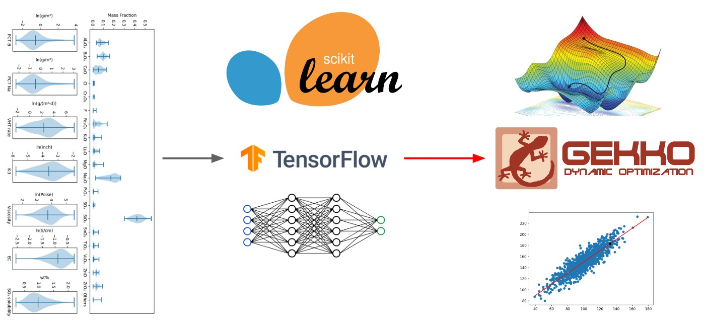
Gradient descent optimization, the optimization method used by Gekko, offers faster optimization time compared to other methods. However, any model or function used with gradient descent must be at least twice differentiable to allow for proper convergence to a solution. Models discussed in this study have this requirement satisfied and are able to be written in mathematical terms that can be interpreted by Gekko. Because of these requirements, each model was individually implemented and rewritten into Gekko. These models are trained in an exterior package, such as Scikit-learn and Tensorflow, and then the trained parameters are imported and used within Gekko. Scikit-learn and Tensorflow are both publicly available packages that implement ML algorithms [
79,
80].
3.1.1. Gaussian Process Regression
Gaussian Process Regression (GPR) is a supervised ML method that can provide prediction values and uncertainty estimates for a given process. The non-parametric method employs Gaussian distributions and pre-defined kernels to approximate an infinite set of functions, and uses the average of these functions after training on the dataset to deliver the predictions [
81]. Based on Bayes’ theorem, GPR estimates and evaluates the probability of a given outcome based on prior knowledge instead of computing exact function parameter values. The process is updated iteratively throughout the training process, and the outcome with the highest probability is used as the final prediction [
82].
The foundational algorithm of a GPR is introduced in Algorithm 1. The algorithm takes in training points (X), target values (y), kernel function, noise, and the sample point as input [
83]. The model outputs the prediction value, the variance for that value, and the log marginal likelihood. The prediction value and variance are used for the actual model prediction and uncertainty, while the log marginal likelihood is used for hyperparameter training. The training algorithm runs in
, while prediction computes in
and variance computes in
.
Of note for this study, the prediction function, line 3 of the GPR Algorithm 1, is calculated by taking the dot product of the pre-computable
values with the diagonal of the kernel function between the sample point and the training set. In order for a model to be used in gradient descent optimization, it must be differentiable; by taking the gradient of this kernel diagonal with respect to the sample point, the gradient of the GPR model can be calculated. As long as the kernel function has a derivative, then the gradient of the model can be calculated and optimized using gradient methods.
| Algorithm 1 The fundamental algorithm for Gaussian Process Regression |
- Input:
X (inputs), y (targets), K (covariance matrix), k (covariance function), (noise level), (test input) -
L := cholesky(K + ) -
-
-
-
-
-
return: (mean), (variance, logp() (log marginal likelihood)
|
The kernel function, or the covariance function, is a function that calculates similarity or closeness between feature points. This function is used to generate and represent infinite functions necessary for a Gaussian process [
81]. The most common kernel function is known as the squared-exponential, or the radial basis function (RBF), shown with other common kernel functions in
Table 1. This specific kernel function has the useful property of being infinitely differentiable. Most kernels include a constant kernel that can be multiplied or added to another or a white noise kernel which would represent noise in the training data set [
79,
83]. Each kernel typically has a length scale parameter which stretches or shrinks the similarity. If one kernel provides inadequate model performance, more kernels can be combined and customized with basic mathematical operations to properly model a process.
GPR offers accurate predictions with uncertainties on most datasets, and can be applied generally with little knowledge of any shape or pattern of the data. The ability to produce uncertainties with those predictions is also useful for better informed decision making and optimization. The method does have drawbacks, however. The most significant problem with GPR is the computation time. As mentioned before, the algorithm runs in . Because of this large time complexity, GPR is not as suitable for data sets larger than a few thousand points. The model is also non-parametric, meaning the necessary parameters needed to describe a model increase with a larger dataset.
In Python, the native language of Gekko, several packages implement training and prediction for GPR. The two most common are Scikit-Learn and GPflow [
79,
84]. Scikit-learn is a general ML package that has several methods; one benefit of this specific implementation is that it stores precomputable parameters and has readable, open-source documentation. GPflow is a Tensorflow based package that is entirely dedicated to GPR; a higher degree of customization and manipulation is available in GPflow when working with the model. The Tensorflow architecture also allows faster computational time for larger datasets. It does not, however, store some precomputable values as Scikit-learn does. Both packages allow for customization of kernel functions.
Gekko creates symbolic equations that are then compiled into byte-code and solved with nonlinear programming solvers. To represent a GPR model in Gekko, the prediction and variance functions are written in terms readable by Gekko. Scikit-learn stores precomputable parameters such as the L matrix and vector from Algorithm 1; these can be imported into a Gekko model and used to predict a function value and uncertainty. As the prediction function is differentiable, this model can be used for gradient-based optimization, and act as an objective function, constraint function, or any necessary intermediate.
3.1.2. Support Vector Regression
Support vector regression (SVR) is a supervised ML regression algorithm based on support vector machines (SVM) [
85]. While SVM is typically used for classification as a maximal margin classifier, SVR is an extension that allows the same method to work in regression applications. SVM is an algorithm that fits hyperplanes, which best separates the training data with the largest margin between the decision border and a set of support vectors. It is originally restricted to feature spaces with linear dependency, while a non-linearly dependent feature space can be transformed using kernel functions such as polynomial and Gaussian kernels [
86]. SVR fits a hyperplane within a predetermined margin to the dataset and uses this plane of best fit for predictions.
Equation (6) is used as the prediction function for the regression model, and is similar to that of GPR, using a kernel based approach. As such, it comes with the same stipulation—the prediction function is differentiable if the kernel function is differentiable. Rather than use the whole training set during prediction, however, SVR selects relevant training points, called support vectors, to factor into the decision function of the regressor. These support vectors are used in conjunction with the optimized vector, bias (b), and kernel function to predict values.
There are several hyperparameters and kernels that can be used to tune SVR. There are four commonly used kernel functions made available in Scikit-learn—the radial basis function (RBF) kernel, linear kernel, polynomial kernel, and the sigmoid kernel. These kernels can be seen in
Table 2. The most common kernel is the RBF kernels. While kernel design is necessary for other algorithms such as GPR, combining or customizing the kernels is not essential for adequate performance.
SVR offers adequate performance and is much less computationally demanding than the other algorithms (e.g., GPR). Rather than use the entire training set in the prediction algorithm like GPR, SVR uses a subset of the training set, the support vectors, for prediction. Because of this, SVR will offer quick predictions no matter the size of the initial training set, while it still has of training time, the prediction is quick at , with m, the number of support vectors used, being less than n.
Drawbacks of SVR include non-robustness, sensitivity to hyperparameter tuning and low flexibility (harder to manipulate) compared to the other advanced algorithms. For instance, it was observed that model performance of SVR is highly dependent on data preparation such as feature scaling and data separation [
87]. In addition, it does not offer prediction intervals, so uncertainty quantification needs to be applied with other packages.
Currently, the most common SVR implementation is through Scikit-learn, based on LIBSVM, a library for SVM, [
79,
85]. Two regression variants exist—
-SVR, where the margin is a hyperparameter, and
-SVR, where the fraction of support vectors is a hyperparameter. Both variants offer similar performance, but solve slightly different optimization problems with different parameters.
Scikit-learn has the necessary precomputed values available to interface to Gekko. These values include the support vectors, the trained matrix, and kernel hyperparameters. Like with GPR, these values are imported into Gekko and used to form the prediction function. While training and validation is still done in Scikit-learn, the SVR is interfaced into Gekko to make the same predictions it would by itself. This allows it to be used to be used for gradient-based optimization.
3.1.3. Artificial Neural Networks
The artificial neural network (ANN) algorithm, inspired by the behavior of biological neurons, contains input, hidden, and output layers. These layers are made of artificial neurons that are interconnected by artificial synapses. The hidden layers include a given number of neurons that take inputs from the input layer, apply mathematical functions, and provide outputs to the output layer. Each neuron weighs the received input values by its associated synapse, where desired outputs are obtained by modifying these weights [
88].The training of a neural network (with back-propagation) is more complex and will not be described in this paper [
89].
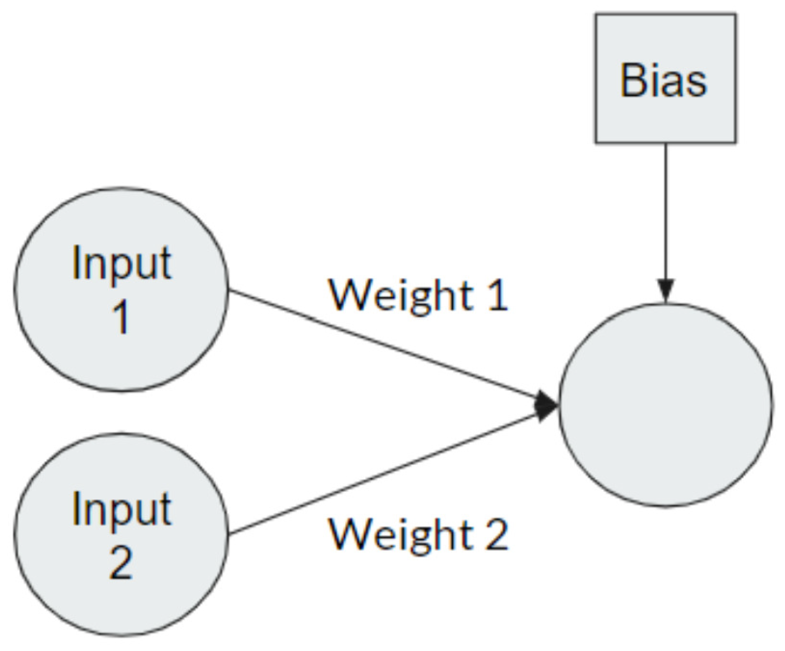
The prediction functions used in both TensorFlow and Scikit-learn neural networks use linear algebra to relate the layers and neurons of the neural network to one another. Each neuron in an input layer has a specific weight that corresponds to an output neuron in the following layer. Each neuron in an output layer also has a corresponding bias value as shown in
Figure 1.
For each neuron connection, there is a bias, weight, and an additional activation function. An additional activation equation, such as the linear rectifier or hyperbolic tangent functions, is generally used to normalize the activation between 0 and 1.
This function is twice differentiable and allows for gradient-based optimization. The prediction functions embedded in TensorFlow and Scikit-learn predict each layer until the final output layer is predicted. Thus, the entire model is twice differentiable and can be implemented into Gekko. The classes that combine Gekko and the model successfully mimic these prediction functions by implementing Equation (11), and are capable of predicting the final output given an input of Gekko variables and a trained model. A trained model is necessary as this provides the needed weights, biases, and activation functions that the model was trained on. These classes are compatible with a wide variety of activation functions included in either Scikit-learn or TensorFlow.
When implementing ANN into the Gekko optimization process, it was found that typical standard scaling functions cannot process Gekko variables. Because the Gekko variables in the optimization model are the original unscaled values, and the models are trained on scaled variables. An additional class was made to scale and unscale Gekko variables. A typical min-max scaling technique is used for this process, similar to the one implemented by Scikit-learn [
79].
Neural networks can be a good choice for a regression model because they provide a fast prediction compared to other ML algorithms like GPR or SVR. In addition, they contain many hyperparameters (number of neurons, number of hidden layers, type of activation function, etc.) with adjustable weights and biases found during training. The performance is dependent on these hyperparameters, and tools such as hyperparameter optimization, improve training results.
Contrarily, there are a few disadvantages to using neural networks. First, incorrect hyperparameter choices can lead to poor training performance. Second, neural networks can have a long training time due to the number of weights and biases that need to be adjusted. Third, typical neural networks do not offer prediction intervals, so they must be paired with an uncertainty method.
3.1.4. Other Methods
Other regression methods have been investigated to determine if they are compatible with Gekko and gradient-based optimization. The most common models are neighborhood based or tree based models that either need to sort the training set or create splits within the training set to produce a regression. These models include K-nearest neighbors, decision tree regressors, random forest regressors, gradient boosted tree regressors, and several others [
79]. Some of these regressors are potentially interesting due to the ability to generate an uncertainty with a point prediction, particularly the gradient boosted tree regressor, which could use a quantile based loss function to generate upper and lower bounds [
90,
91,
92].
However, these regressors have been determined to be infeasible to use with the Gekko optimization package. In order for regression to be made in the optimization package, the models need to be broken down and have first and second derivative information made available. The nature of these models leads to a piece-wise predictor function that does not have a continuous first and second derivative function. For nearest neighbors methods, the distance metric vector for the training set would need to be sorted on every call to the prediction function, yielding piece-wise structure. Likewise, for tree based methods, splits are made within the training set that do not allow for first and second derivatives [
93,
94].
It may be possible for some methods to be interfaced into Gekko. Continuous approximations for these models may exist, as suggested in this paper [
95]. However, in the current state of Gekko and these models, they cannot be interfaced and integrated into the optimization package.
3.1.5. Example Benchmark Problem
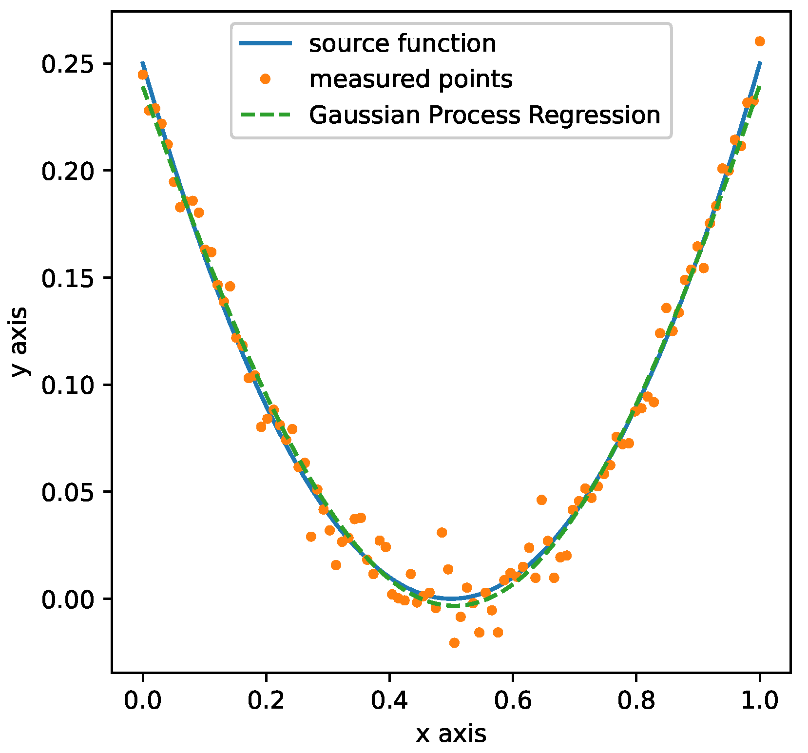
Presented here is an example of using these tools to find the minimum of an objective function. A trivial benchmark function, Equation (12), is used to generate 100 random normally distributed data-points that represent the source function. These data are then used to train and validate a GPR; both the source function and the GPR are then used to find the minimum value of the function. This GPR model has a high performance with an
of 0.981. Source function, generated data, and the GPR model are visualized in
Figure 2.
As an optimization tool, Gekko can calculate the minimum of a provided source function as long as it is described in algebraic terms. If only data is available, however, a ML model can be used to fit the data, and then imported into Gekko, as seen in this example. Below, in Listings 1 and 2, both source function and GPR model are used in Gekko to find the minimum of the function.
| Listing 1. Optimization with Source Function. |
 |
| Listing 2. Optimization with Gaussian Process Regression. |
 |
In
Table 3, the results for this benchmark problem are reported as the converged solution, objective function value, and solve time. Due to data generation with simulated randomness and regression modeling, the solution and objective are not the exact same as the source function optimization. Regardless, this simple case shows that optimization in Gekko is possible when an objective function is a trained ML model. ML models can also be used as intermediate functions and constraints, not just objective functions. Additionally, this exercise is repeatable with all other models previously mentioned.
3.2. Uncertainty Quantification
Uncertainty quantification is often necessary with predictions and estimates to make better informed decisions. For the LAW optimization problem, prediction intervals are used to distance constrained values from the constraint limits. The significance level of the prediction intervals indicate how likely future predictions would fall within the interval; a 95% prediction interval includes 95% of all future values. Thus, a higher significance level results in a larger uncertainty. The following uncertainty methods have been successfully implemented into the Gekko environment with the ML methods. These methods were chosen due to their prevalence in the literature and the ability to pair them with any ML model.
3.2.1. Delta Method
One method of uncertainty uses an equation to calculate a simultaneous upper confidence interval (SUCI). The SUCI works similar to the significance level. A 95% SUCI ensures that there is 95% confidence that the property produced will satisfy the requirements, or lie within the uncertainty boundary. The formula for a
confidence level SUCI on an unlimited number of compositions,
g, using the Working-Hotelling approach is given by [
96], and shown in Equation (13).
where:
s is the root mean squared error associated with the model,
p is the number of model parameters,
is the
th-percentile of the
F-distribution with
p and
degrees of freedom,
n is the number of datapoints used in model fitting,
g is the composition vector, and
G is the matrix of composition vectors used in model development [
31].
This method of uncertainty quantification has been extended and applied to other nonlinear regression models, and is commonly known as the delta method. Any prediction model that can be considered a nonlinear regression model can be used with the delta method. The method can be used to calculate both confidence intervals and prediction intervals. The prediction interval equation is shown in Equation (14).
This method was implemented into Gekko by writing Equation (14) into Gekko legible terms. Training data from any model would need to be saved as the G matrix, and used for future predictions and prediction intervals.
3.2.2. Conformal Method
Conformal prediction (CP) is a model agnostic method that produces well-calibrated uncertainty band for each prediction [
97]. CP uses a predefined nonconformity function to score each training point on the level of conforming, or the similarity to other points of the same label or value. This conformity score serves as a metric in comparing one data point to the rest of the set. A significance level is provided to the calculations to allow for proper calibration. The significance level and conformity scores are used to create an interval at a given significance level—for example, 95%. At the 95% significance level, 95% of the data falls within those prediction intervals, which would indicate proper calibration for an uncertainty method.
The CP method is implemented by the nonconformist package [
98]. It can use any model as the underlying model for inductive conformal predictions. A calibration set must be set aside to calculate the uncertainty—for this paper, a 20% split of the training set was used. The model is then trained, and then the uncertainty is calibrated to provide a constant prediction interval. This trained model and constant prediction interval can be interfaced into Gekko for future predictions with intervals.
3.2.3. Ensemble Method
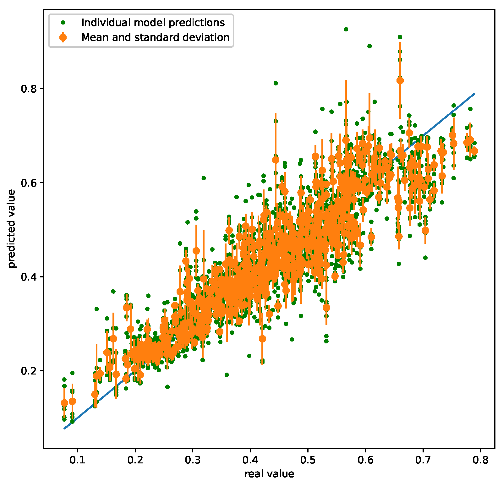
Ensemble methods are techniques that make use of training multiple models to improve the accuracy of the prediction and provide an uncertainty. This is useful for calculating an uncertainty for models with no built in uncertainty method. There are many different ensemble methods; two described in this paper are bootstrapping and resampling.
Bootstrapping is accomplished by training n models on n different training sets. The training data for each model is randomly selected with replacement, meaning the same data point can be used in multiple training sets. Because the training data is randomly selected, each of the n models’ predictions will be slightly different. To implement bootstrapping, n different training sets are created and n different models are trained from a corresponding training set. Thus, each time a prediction is made, an array of n predictions is actually made. The mean value is the ‘true’ prediction for this method and the standard deviation is calculated from the array. The standard deviation is then multiplied by 1.96 or 1.645 to provide an uncertainty with a 95% or 90% significance level, respectively.
Resampling is similar to bootstrapping; however, instead of training
n models on
n training sets,
n models are trained on 1 training set. This method is more effective with neural networks because each training of a new model on the same dataset provides a different set of weights and biases. Resampling is implemented by training multiple models on one training set. An array of predictions is made from these models and the same technique as bootstrapping is followed to calculate a true prediction and uncertainty. Seen in
Figure 3 is an example of an ensemble method of uncertainty using multiple models.
Implementing any form of ensemble uncertainty only requires training multiple models, so implementation into Gekko involves multiple models rather than a single model. As expected, an ensemble with more models demands more computational power as there are more models to run.
3.2.4. Model Specific Uncertainty Methods
Some uncertainty methods are model specific; they can only be used with an appropriate model. Presented here are two model specific uncertainty methods explored; Gaussian uncertainty and a loss function trained neural network.
Gaussian Process Regression is a unique model in that in inherently calculates uncertainty with the prediction. As explained previously, GPR uses kernel functions to approximate an infinite amount of smooth functions that could fit the training points. By using the mean of these functions, a prediction can be achieved; likewise, by using other population statistics, such as standard deviation, a prediction uncertainty can also be calculated.
A newer method for determining uncertainty, specifically designed for neural networks, takes advantage of implementing a custom loss function into TensorFlow. A loss function is a method of expressing how well a model represents the data. Standard loss functions include mean squared error and mean absolute error. These loss functions minimize the sum square of the difference between the model’s prediction value and the true value. Although they work well to find model parameters that represent the data accurately, they provide no uncertainty. Instead of using one of these loss functions, a loss function designed by Dr. Robert Kubler can be implemented [
99] to include model uncertainty. This loss function is defined below.
Kubler’s loss function includes portions of the mean squared error in order to measure how well the model represents the true property. Unlike typical ANN loss functions however, this loss function also includes the standard deviation, . Thus, when the model makes a prediction, it outputs a standard deviation in addition to the property prediction. This standard deviation represents the model’s uncertainty in the new prediction. This is advantageous because it provides an uncertainty along with the prediction, and is faster than other methods like ensemble methods.
There are other models with uncertainty methods specific to them. One such method is the pairing of a gradient descent tree booster [
91] with a loss function, as was done with neural networks. However, due to tree-based regressors not being compatible with the framework of Gekko, this option is not implemented.
4. Results and Discussion
Currently, partial quadratic mixture (PQM) models are commonly used to predict constrained properties as a function of glass composition [
31]. A systematic evaluation of Hanford LAW loading in glasses formulated using these PQM based models were conducted previously [
4]. The PQM model is similar to a linear regression model, with certain compositions and engineered features used as inputs. The performance and uncertainty of these models are adequate and have been validated experimentally, however replacing these with well trained machine learning models can lead to more accurate results and more confidence in the property prediction as well as the overall problem solution (e.g., higher waste loading and/or closer to true optimal glass compositions). In addition, computation time is also evaluated during the testing of these models, because reducing computation time can significantly decrease the total time during case evaluation of thousands of waste batches. PQM results are presented along with ML model results.
For adequate comparison, each of the models are fitted with five-fold cross validation. The dataset has 566 glass composition entries for the electrical conductivity property, with 20 composition features. For each cross validation, an 80–20 random split is used on the dataset; 80% of the data was sectioned off for training purposes, and 20% for testing. For uncertainty comparison, the 90% prediction interval is calculated for each model and UQ method combination; some UQ methods require another split of data be set aside during model training. A dotted line is present on all graphs showing PQM performance for comparison. Results presented in this study includes regression performance on the provided data-set, uncertainty calibration curves, property values with uncertainty values, optimization solve time, and the final waste loading. The objective of the optimization problem is to maximize final waste loading; doing so without giving up certainty or computational time is desired. For the ensemble methods, 20 models are trained and combined for each cross validation run, except for GPR due to the longer computation time, where only 5 models are computed.
4.1. Training Performance
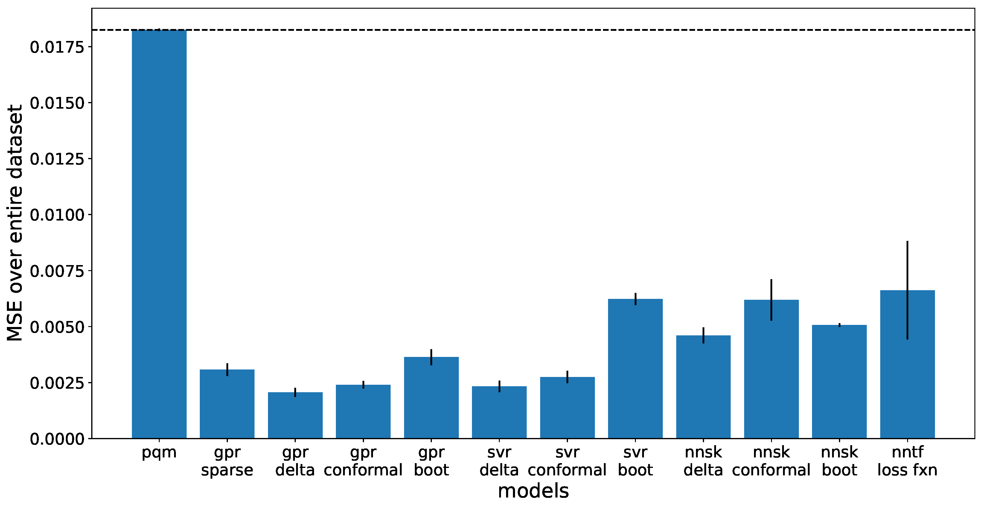
Mean squared error (MSE) is used as a comparison metric between the linear PQM model and the non-linear ML models. The MSE is taken over the entire dataset of 566 glass compositions. As seen in
Figure 4, Each ML model performs significantly better than the PQM model. The highest performing models include the GPR with delta or conformal uncertainty.
As mentioned previously, uncertainty methods change how each model is trained by selecting a different portion of the dataset. Each split is randomly generated. For conformal Prediction uncertainty, a 20% split of the data needs to be taken out as a calibration set, decreasing performance. For bootstrap uncertainty, only half of the training set is used to train each model. For Gaussian uncertainty, a sparse GPR must be used for the sake of computational time, meaning only a small portion, 20%, of the dataset is used for training. All models train better when there is more data to train from, so restricting some data evidently decreases performance. The delta uncertainty method does not require any training data to be removed, so it represents the best trained models without removing additional training data.
4.2. Uncertainty Calibration
UQ and verification of the calculated prediction intervals is a difficult task. Intervals can be underconfident if they are too small and overconfident if they are too wide; in either case, the prediction intervals no longer represent a realistic prediction and become unreliable to use. In order for an UQ method to be valid, it needs to encompass the portion of data that it represents; a 90% prediction interval needs to guarantee that 90% of the dataset falls within those predictions with attached intervals. While a lower uncertainty is more desirable for this optimization application, the lower uncertainty needs to be justified. The metric used for uncertainty calibration is the root mean squared calibration error (RMSCE) [
100]. A lower RMSCE indicates a more calibrated uncertainty measurement.
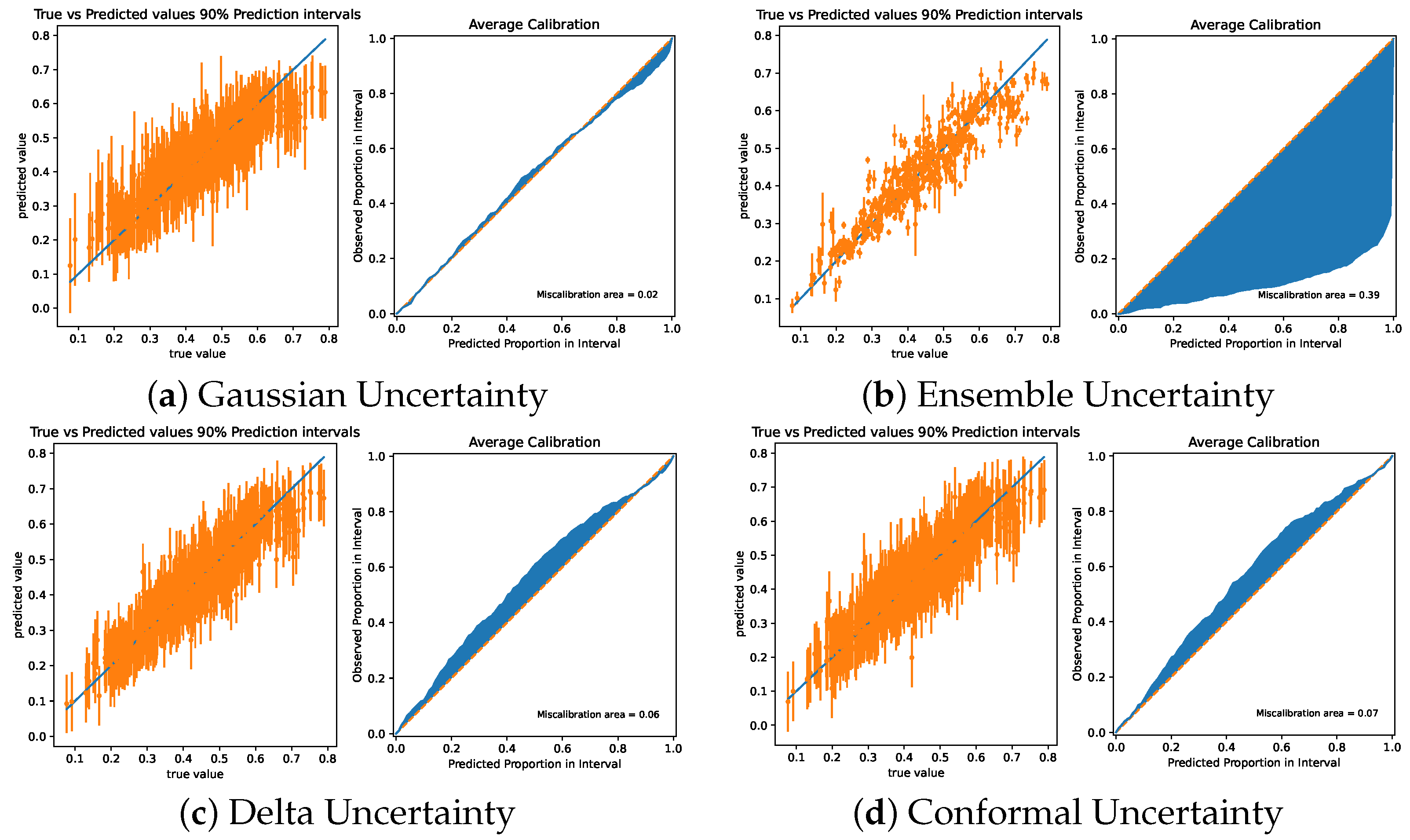
Four characteristic calibration graphics can be found in
Figure 5. Each graphic represents the width of prediction intervals over the dataset as well as the coverage of these intervals. GPR is used as the model to generate these figures. The PQM model with its delta uncertainty method has an RMSCE of 0.0538. Other low RMSCE values are found in the GPR and SVR delta uncertainty method, with an RMSCE of 0.06. conformal uncertainty and delta uncertainty is slightly overconfident for all models. Gaussian uncertainty is well calibrated, with an RMSCE of 0.02. Ensemble uncertainty methods are under confident in most predictions.
These results show that the delta uncertainty method has the lowest RMSCE of the model-agnostic methods, meaning it is the best suited method for UQ in this application. Gaussian and conformal uncertainty methods are also well calibrated. As ensemble uncertainty methods are underconfident, they can’t reliably be used for UQ; the intervals provided by these methods are too small and may not include the measurement. Gaussian uncertainty requires the use of a sparse GPR; although it has a lower RMSCE, it also has a lower training performance. Underconfidence in UQ can lead to property uncertainties being too low and the optimized composition being too close to constraint boundaries; overconfidence can cause the numerical solver to fail and not converge on the solution, as the UQ intervals may be wider than the constraints.
4.3. Optimization Results
The optimization results for the simplified LAW optimization problem are provided here. The objective (waste loading), solve time, constrained property (Electrical Conductivity) and its associated uncertainty are shown on
Figure 6,
Figure 7,
Figure 8 and
Figure 9. Each model was paired with each compatible UQ method and used on the optimization problem to get the results presented.
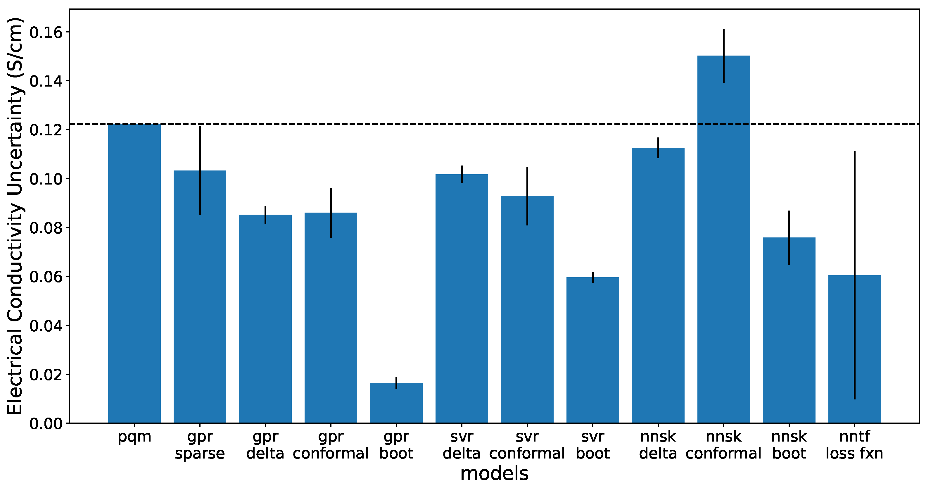
Figure 6 shows results of the 90% prediction interval uncertainty for the electrical conductivity property. These graphs show the width of the 90% interval at the optimal solution composition. The lowest calculated uncertainties can be found in the ensemble of neural networks and the neural network trained with a quantile loss function. However, these uncertainties are less calibrated and more underconfident as described in the previous section, which means they may not be as reliable or trustworthy as the other methods. The lowest calculated uncertainty with highest calibration is found in the delta Uncertainty method with the GPR. The SVR models as well as the ANN with delta uncertainty also had a lower uncertainty than the PQM model.
The electrical conductivity property result is presented in
Figure 7. Typically, a higher EC value is associated with a higher waste loading for the simplified optimization problem. As the uncertainty interval is used to distance the electrical conductivity from constraint bounds, a smaller uncertainty interval allows the property models to approach the upper constraint limit and reach a higher waste loading. Running the optimization problem without uncertainty leads to convergence to the upper limit and a higher waste loading in every case.
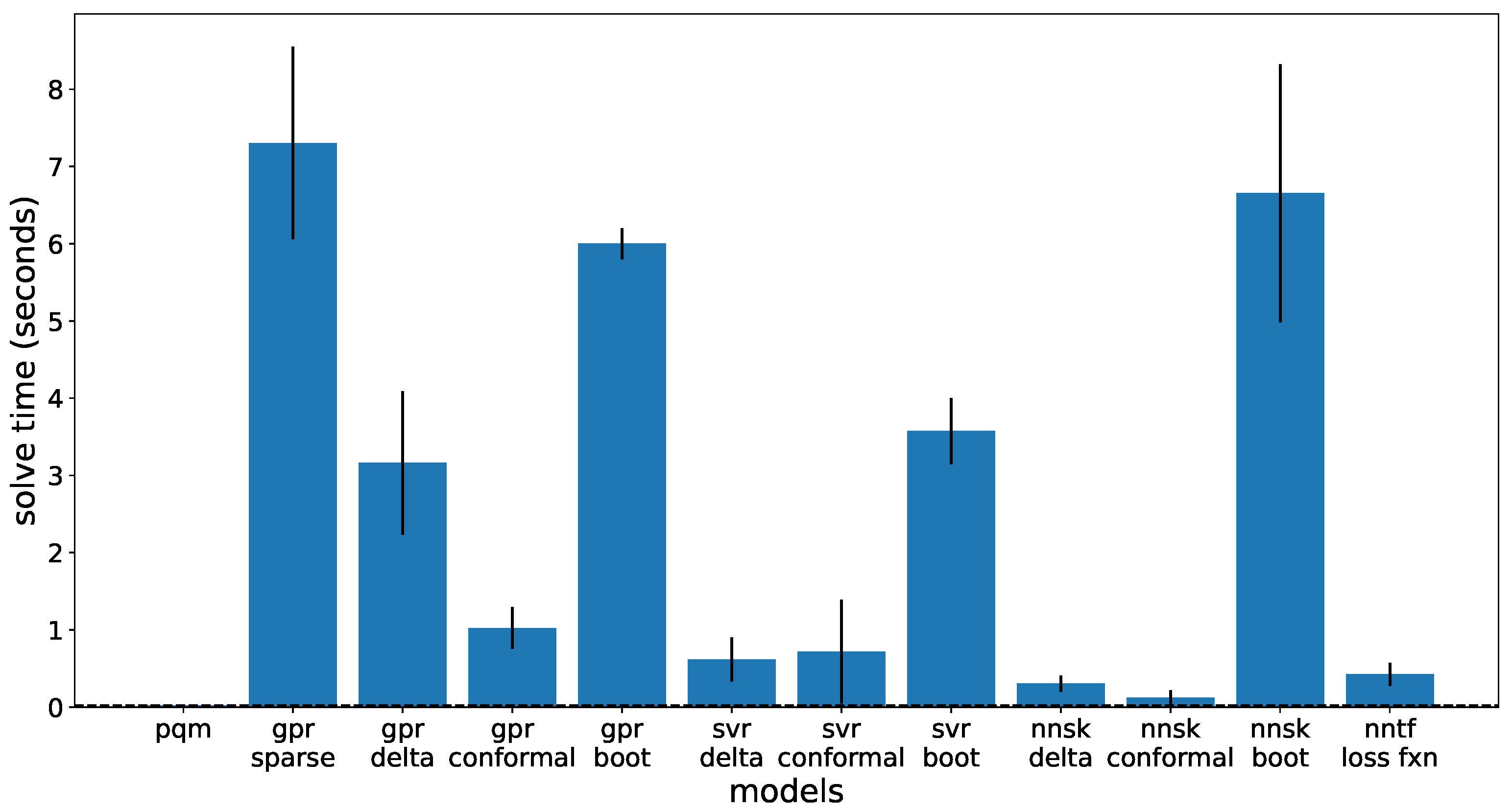
Figure 8 depicts the amount of time to solve the simplified optimization problem. These results were calculated on a personal computer with a 10th gen Intel core i5 processor, so no excessive resources were allocated to run the optimization problem. As the PQM model is similar to a linear regression method, the calculation time is quick (hundredths of a second). The next quickest are the non-bootstrapped neural networks; neural networks are typically fast at predictions due to the simple linear algebra, so this was expected. Both the PQM and neural network models are also parametric models; parametric models do not depend on the size of the training set and are fast because of their smaller scale. The others are non-parametric. SVR methods are the next fastest algorithm for this problem as the support vectors do not represent the entire training set leading to a faster calculation time. GPR tends to be the slowest due to using most of the training set, or, for sparse GPR, running through the computationally large Gaussian uncertainty method. The other slow method is the ensemble of ANN; as this is running 20 neural network calculations, this is expected. In comparison to previous optimization attempts with CasADi [
40], these results are promising. CasADi optimization runs took up to 5 min with GPR due to a different solving method. Having a quicker computational time demonstrates that these models can serve as an effective replacement to more traditional models without a tradeoff in solve time.
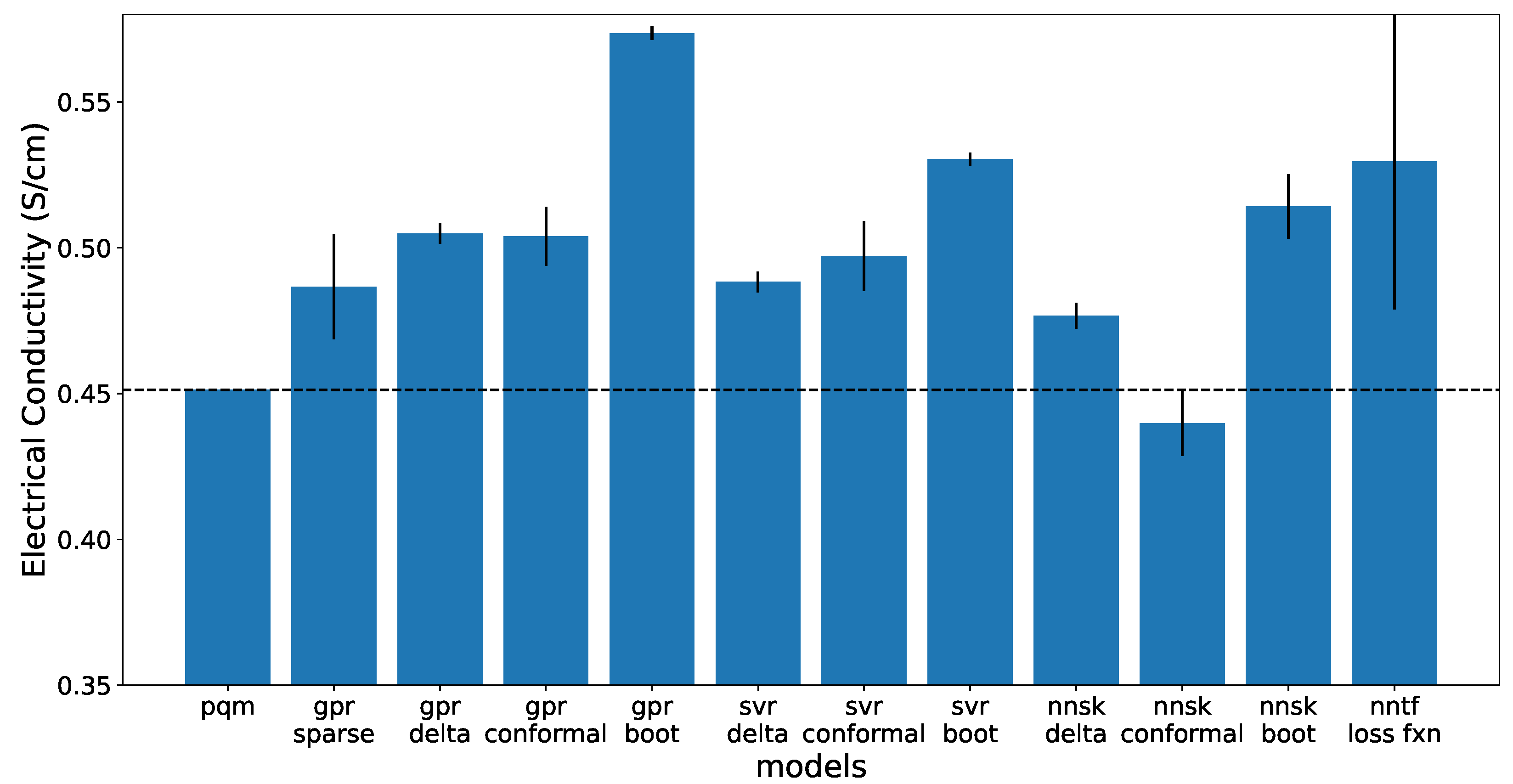
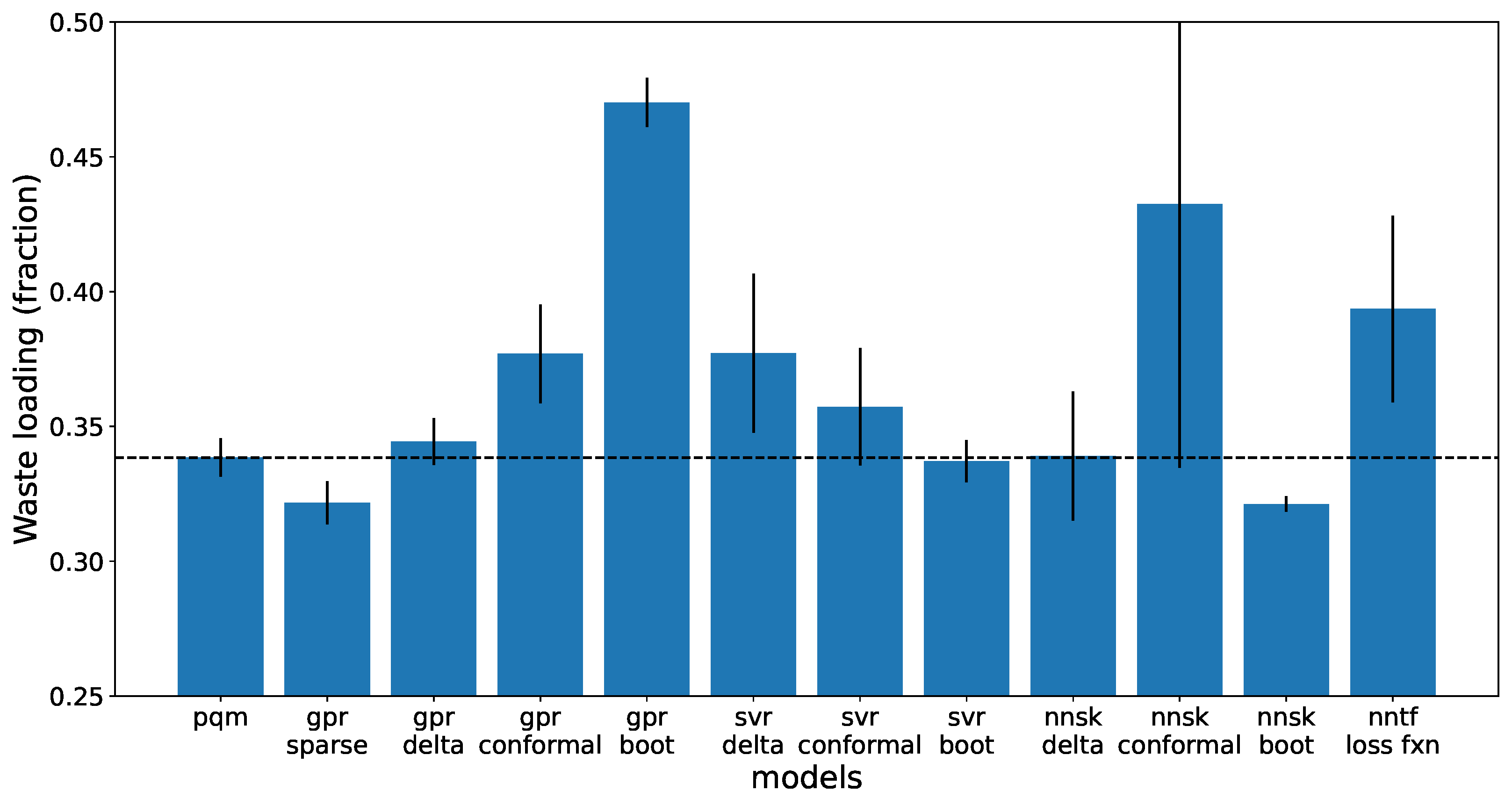
Shown in
Figure 9 is the optimization target, the waste loading. By optimizing different input parameters like composition of glass formers, the numerical optimization routine used by Gekko tries to maximize waste loading. The conformal SVR as well as the delta uncertainty ANN have the highest waste loading, but also have a large variation between the different training splits. Most other models also have a slightly higher average waste loading than a PQM with a slightly larger variance.
For this simplified problem, the objective was to show that ML models with proper UQ could be used to achieve a higher waste loading during numerical optimization in Gekko. Most models trained had higher regression performance than the PQM model, shown in
Figure 4. As shown in
Figure 9, most model and method pairings did result in a higher waste loading; while some model and methods may be questionable due to the high variation between cross validation (SVR delta, ANN conformal, and ANN loss function), others have consistent results. Additionally, the UQ methods presented are as calibrated in as the PQM model and can produce lower uncertainties represented in
Figure 6. For this application, the GPR model with conformal UQ method performs best in all categories judged, with several other model and method pairings performing similarly.
5. Conclusions
In this study, well known ML algorithms are interfaced with the optimization suite, Gekko, in Python. The goal was to see if these ML algorithms, such as GPR, SVR, and ANN could be used in a proof-of-principle optimization problem. Similar attempts have been made before, but few have directly used these algorithms with a gradient-based approach of optimization. Additionally, various methods of uncertainty quantification are also explored and paired with these models: these methods include ensemble methods, model-specific methods, conformal predictions, and the delta method.
These tools are used on an example case study problem, involving the optimization of glass composition to have maximum waste loading in nuclear waste vitrification. Using a simplified optimization problem and comparing to the previous PQM model, the tools developed in this study are capable of achieving higher waste loading at a lower prediction uncertainty. Additionally, the computation time for these tools are compared, with the added benefit of a higher performance of predicting the data. More work remains to be done in the case of testing these models on the full scale version of this problem.
For the Hanford LAW problem, the best applicable model and method combination was determined to be the GPR with conformal Uncertainty. GPR tends to have the best performance among the models examined, as well as a better performance than the PQM model. Additionally, the uncertainty calculated is smaller than that of the PQM model, yet still retains a confident calibration. Most importantly, the waste loading is shown to have noticeably increased when using this model and method combination. For this simplified case study problem, where electrical conductivity was the only property modelled and constrained, GPR with conformal Uncertainty provides the most promising results. Other models and methods, like GPR with delta Uncertainty and some SVR models also perform well.
This case study is just one example of how ML can be used in a physics based optimization environment. Previous models can be replaced or supplemented by higher performing models, without the consequence of slower optimization. Additionally, uncertainty quantification allows these models to reflect a realistic outcome rather than just providing a pointwise prediction. Future work for this endeavor includes investigation into other regression models, further study of UQ, and application in other areas of interest, such as other optimization problems or dynamic control. As Gekko is a public platform, these tools may be used for other applications and problems that require optimization and ML. Validation of the optimization results is future work with the pending startup of the waste melter at the Hanford Waste Treatment and Immobilization Plant. The vitrification plant will operate with two 300-ton melters in the Low Activity Waste Facility. Glass samples from the vitrification plant can provide additional data to refine the machine learned models and optimization strategy.
This effort is an example of bringing modern computational tools like ML and UQ and applying them in industries in need of higher precision and accuracy with their modeling tools. Nuclear waste vitrification at Hanford is a good application of how numerical optimization can be paired with ML and UQ to make better informed decisions in the plant during operation. These decisions need to be made fast and be reliable, as the 20 dimensional input space from the constantly varying glass composition can be challenging to predict with older tools alone. ML can improve waste glass formulation over traditional models, leading to a true maximum of waste loading. This study shows that higher performance and higher confidence is possible without sacrificing computation time. In a complex problem like the one presented, the improved speed of the new methods enable detailed sensitivity analysis. During plant operation, these models can be used for faster decision and optimization while the models learn from each new glass composition. This case study shows that ML and UQ with numerical optimization has a place in other processing plants with similar challenges.
Author Contributions
Conceptualization, X.L., J.V. and J.H.; methodology, L.L.G., K.M., X.L., J.V. and J.H.; software, L.L.G. and K.M.; validation, L.L.G., K.M. and X.L.; resources, X.L. and J.V.; data curation, X.L.; writing—original draft preparation, L.L.G., K.M., X.L., J.R. and J.V.; writing—review and editing, X.L., J.R. and J.V.; visualization, L.L.G. and K.M.; supervision, X.L., J.V. and J.H.; project administration, J.V.; funding acquisition, X.L. and J.V. All authors have read and agreed to the published version of the manuscript.
Funding
Pacific Northwest National Laboratory is a multi-program national laboratory operated for the U.S. Department of Energy by Battelle Memorial Institute under Contract DE-AC06-76RL01830. This project was funded as a subcontract to Brigham Young University to develop machine learning methods for Gekko Optimization Suite in support of nuclear waste modeling and loading optimization.
Institutional Review Board Statement
Not applicable.
Informed Consent Statement
Not applicable.
Data Availability Statement
Acknowledgments
The authors are grateful for the support by the U.S. Department of Energy (DOE), Office of River Protection Waste Treatment and Immobilization Plant (WTP) Project. We would like to thank Zachary D Weller (PNNL) and José Marcial (PNNL) for reviewing the manuscript, Charmayne E. Lonergan (PNNL), Renee L. Russell (PNNL), William C. Eaton (PNNL) and Albert Kruger (ORP) for programmatic support during the conduct of this work.
Conflicts of Interest
The authors declare no conflict of interest. The funders had no role in the design of the study; in the collection, analyses, or interpretation of data; in the writing of the manuscript; or in the decision to publish the results.
References
- Beal, L.D.; Hill, D.C.; Martin, R.A.; Hedengren, J.D. Gekko optimization suite. Processes 2018, 6, 106. [Google Scholar] [CrossRef]
- Waechter, A.; Biegler, L.T. On the Implementation of a Primal-Dual Interior Point Filter Line Search Algorithm for Large-Scale Nonlinear Programming. Math. Program. 2006, 106, 25–57. [Google Scholar] [CrossRef]
- Hedengren, J.; Mojica, J.; Cole, W.; Edgar, T. APOPT: MINLP Solver for Differential and Algebraic Systems with Benchmark Testing. In Proceedings of the INFORMS National Meeting, Phoenix, AZ, USA, 14–17 October 2012. [Google Scholar]
- Lu, X.; Kim, D.S.; Vienna, J.D. Impacts of constraints and uncertainties on projected amount of Hanford low-activity waste glasses. Nucl. Eng. Des. 2021, 385, 111543. [Google Scholar] [CrossRef]
- Almeida, L.; Duprez, M.; Privat, Y.; Vauchelet, N. Mosquito population control strategies for fighting against arboviruses. Math. Biosci. Eng. 2019, 16, 6274–6297. [Google Scholar] [CrossRef] [PubMed]
- Hill, D.; Martin, A.; Martin-Nelson, N.; Granger, C.; Memmott, M.; Powell, K.; Hedengren, J. Techno-economic sensitivity analysis for combined design and operation of a small modular reactor hybrid energy system. Int. J. Thermofluids 2022, 16, 100191. [Google Scholar] [CrossRef]
- Verleysen, K.; Parente, A.; Contino, F. How does a resilient, flexible ammonia process look? Robust design optimization of a Haber-Bosch process with optimal dynamic control powered by wind. Proc. Combust. Inst. 2022, in press. [Google Scholar] [CrossRef]
- Park, Y.M.; Tun, Y.K.; Han, Z.; Hong, C.S. Trajectory Optimization and Phase-Shift Design in IRS-Assisted UAV Network for Smart Railway. IEEE Trans. Veh. Technol. 2022, 71, 11317–11321. [Google Scholar] [CrossRef]
- Mowbray, M.; Vallerio, M.; Perez-Galvan, C.; Zhang, D.; Chanona, A.D.R.; Navarro-Brull, F.J. Industrial data science—A review of machine learning applications for chemical and process industries. React. Chem. Eng. 2022, 7, 1471–1509. [Google Scholar] [CrossRef]
- Zhou, F.; Li, Y.; Wang, W.; Pan, C. Integrated energy management of a smart community with electric vehicle charging using scenario based stochastic model predictive control. Energy Build. 2022, 260, 111916. [Google Scholar] [CrossRef]
- Martin, R.A.; Gates, N.S.; Ning, A.; Hedengren, J.D. Dynamic Optimization of High-Altitude Solar Aircraft Trajectories Under Station-Keeping Constraints. J. Guid. Control Dyn. 2019, 42, 538–552. [Google Scholar] [CrossRef]
- Hansen, B.; Tolbert, B.; Vernon, C.; Hedengren, J.D. Model predictive automatic control of sucker rod pump system with simulation case study. Comput. Chem. Eng. 2019, 121, 265–284. [Google Scholar] [CrossRef]
- Nubli, H.; Sohn, J.M.; Prabowo, A.R. Layout optimization for safety evaluation on LNG-fueled ship under an accidental fuel release using mixed-integer nonlinear programming. Int. J. Nav. Archit. Ocean Eng. 2022, 14, 100443. [Google Scholar] [CrossRef]
- Colburn, H.A.; Peterson, R.A. A history of Hanford tank waste, implications for waste treatment, and disposal. Environ. Prog. Sustain. Energy 2021, 40, e13567. [Google Scholar] [CrossRef]
- Bernards, J.K.; Hersi, G.A.; Hohl, T.M.; Jasper, R.T.; Mahoney, P.D.; Pak, N.K.; Reaksecker, S.D.; Schubick, A.J.; West, E.B.; Bergmann, L.M.; et al. River Protection Project System Plan; U.S. Department of Energy: Washington, DC, USA, 2020. [Google Scholar]
- Vienna, J.D. Nuclear waste vitrification in the United States: Recent developments and future options. Int. J. Appl. Glass Sci. 2010, 1, 309–321. [Google Scholar] [CrossRef]
- Hill, R.C.P.; Reynolds, J.G.; Rutland, P.L. A Comparison of Hanford and Savannah River Site High-Level Wastes; American Nuclear Society: La Grange Park, IL, USA, 2011; Volume 1, pp. 114–117. [Google Scholar]
- Bolling, S.D.; Reynolds, J.G.; Ely, T.M.; Lachut, J.S.; Lamothe, M.E.; Cooke, G.A. Natrophosphate and kogarkoite precipitated from alkaline nuclear waste at Hanford. J. Radioanal. Nucl. Chem. 2020, 323, 329–339. [Google Scholar] [CrossRef]
- Daniel, R.; Peterson, R.; Westman, B.; Burns, C. Impact of dilution-induced precipitates on the filtration of Hanford liquid tank wastes. Sep. Sci. Technol. 2022, 57, 2635–2651. [Google Scholar] [CrossRef]
- Dixon, D.R.; Westesen, A.M.; Hall, M.A.; Stewart, C.M.; Lang, J.B.; Cutforth, D.A.; Eaton, W.C.; Peterson, R.A. Vitrification of Hanford Tank Wastes for Condensate Recycle and Feed Composition Changeover Testing; Washington River Protection Solutions, LLC: Richland, WA, USA, 2021. [Google Scholar] [CrossRef]
- McGinnis, C.P.; Welch, T.D.; Hunt, R.D. Caustic leaching of high-level radioactive tank sludge: A critical literature review. Sep. Sci. Technol. 1999, 34, 1479–1494. [Google Scholar] [CrossRef]
- Pegg, I.L. Behavior of technetium in nuclear waste vitrification processes. J. Radioanal. Nucl. Chem. 2015, 305, 287–292. [Google Scholar] [CrossRef]
- Reynolds, J.G. The apparent solubility of aluminum (III) in Hanford high-level waste. J. Environ. Sci. Health Part A 2012, 47, 2213–2218. [Google Scholar] [CrossRef]
- Reynolds, J.G.; Cooke, G.A.; Herting, D.L.; Warrant, R.W. Salt Mineralogy of Hanford High-Level Nuclear Waste Staged for Treatment. Ind. Eng. Chem. Res. 2013, 52, 9741–9751. [Google Scholar] [CrossRef]
- Reynolds, J.; Tardiff, B. A Rothmund–Kornfeld model of Cs+–K+–Na+ exchange on spherical resorcinol-formaldehyde (sRF) resin in Hanford nuclear waste. J. Radioanal. Nucl. Chem. 2016, 309, 813–818. [Google Scholar] [CrossRef]
- Russell, R.; Snow, L.; Peterson, R. Methods to Avoid Post-Filtration Precipitation in Treatment of High-Level Waste. Sep. Sci. Technol. 2010, 45, 1814–1821. [Google Scholar] [CrossRef]
- Vienna, J.D. Compositional models of glass/melt properties and their use for glass formulation. Procedia Mater. Sci. 2014, 7, 148–155. [Google Scholar] [CrossRef]
- Kruger, A.A.; Cooley, S.K.; Joseph, I.; Pegg, I.L.; Piepel, G.F.; Gan, H.; Muller, I. Final Report—ILAW PCT, VHT, Viscosity, and Electrical Conductivity Model Development, VSL-07R1230-1; USDOE Office of Environmental Management (EM): Washington, DC, USA, 2013. [Google Scholar] [CrossRef]
- Kruger, A.A.; Kim, D.S.; Vienna, J.D. Preliminary ILAW Formulation Algorithm Description, 24590 Law RPT-RT-04-0003, rev. 1. Hanford Tank Waste Treatment and Immobilization Plant; Office of Scientific and Technical Information, U.S. Department of Energy: Oak Ridge, TN, USA, 2013. [Google Scholar] [CrossRef]
- Kruger, A.A.; Piepel, G.F.; Landmesser, S.M.; Pegg, I.L.; Heredia-Langner, A.; Cooley, S.K.; Gan, H.; Kot, W.K. Final Report—IHLW PCT, Spinel T1%, Electrical Conductivity, and Viscosity Model Development, VSL-07R1240-4; Hanford Site (HNF): Richland, WA, USA, 2013. [Google Scholar] [CrossRef]
- Vienna, J.; Heredia-Langner, A.; Cooley, S.; Holmes, A.; Kim, D.S.; Lumetta, N. Glass Property-Composition Models for Support of Hanford WTP Law Facility Operation; Pacific Northwest National Lab. (PNNL): Richland, WA, USA, 2022. [Google Scholar] [CrossRef]
- Vienna, J.; Piepel, G.; Kim, D.S.; Crum, J.; Lonergan, C.; Stanfill, B.; Riley, B.; Cooley, S.; Jin, T. 2016 Update of Hanford Glass Property Models and Constraints for Use in Estimating the Glass Mass to be Produced at Hanford by Implementing Current Enhanced Glass Formulation Efforts; Pacific Northwest National Lab. (PNNL): Richland, WA, USA, 2016. [Google Scholar] [CrossRef]
- Lumetta, N.; Kim, D.S.; Vienna, J. Preliminary Enhanced Law Glass Formulation Algorithm; Pacific Northwest National Lab. (PNNL): Richland, WA, USA, 2022. [Google Scholar] [CrossRef]
- Liu, H.; Fu, Z.; Yang, K.; Xu, X.; Bauchy, M. Machine learning for glass science and engineering: A review. J. Non-Cryst. Solids X 2019, 4, 100036. [Google Scholar] [CrossRef]
- Hu, G.; Pfingsten, W. Data-driven machine learning for disposal of high-level nuclear waste: A review. Ann. Nucl. Energy 2023, 180, 109452. [Google Scholar] [CrossRef]
- Le Tallec, X.; Zeghal, S.; Vidal, A.; Lesouëf, A. Effect of influent quality variability on biofilter operation. Water Sci. Technol. 1997, 36, 111–117. [Google Scholar] [CrossRef]
- Eksteen, J.; Frank, S.; Reuter, M. Dynamic structures in variance based data reconciliation adjustments for a chromite smelting furnace. Miner. Eng. 2002, 15, 931–943. [Google Scholar] [CrossRef]
- Cutler, C.; Eksteen, J. Variance propagation in toll smelting operations treating multiple concentrate stockpiles. J. S. Afr. Inst. Min. Metall. 2006, 106, 221–227. [Google Scholar]
- Zhang, H.; Wang, L.; Han, Z.; Liu, Q.; Wang, W. A robust data reconciliation method for fast metal balance in copper industry. Control Eng. Pract. 2020, 105, 104648. [Google Scholar] [CrossRef]
- Andersson, J.A.; Gillis, J.; Horn, G.; Rawlings, J.B.; Diehl, M. CasADi: A software framework for nonlinear optimization and optimal control. Math. Program. Comput. 2019, 11, 1–36. [Google Scholar] [CrossRef]
- Bynum, M.L.; Hackebeil, G.A.; Hart, W.E.; Laird, C.D.; Nicholson, B.L.; Siirola, J.D.; Watson, J.P.; Woodruff, D.L. Pyomo–Optimization Modeling in Python, 3rd ed.; Springer Science & Business Media: Berlin/Heidelberg, Germany, 2021; Volume 67. [Google Scholar]
- Dunning, I.; Huchette, J.; Lubin, M. JuMP: A modeling language for mathematical optimization. SIAM Rev. 2017, 59, 295–320. [Google Scholar] [CrossRef]
- Houska, B.; Ferreau, H.J.; Diehl, M. ACADO toolkit—An open-source framework for automatic control and dynamic optimization. Optim. Control Appl. Methods 2011, 32, 298–312. [Google Scholar] [CrossRef]
- Verschueren, R.; Frison, G.; Kouzoupis, D.; Frey, J.; Duijkeren, N.V.; Zanelli, A.; Novoselnik, B.; Albin, T.; Quirynen, R.; Diehl, M. acados—A modular open-source framework for fast embedded optimal control. Math. Program. Comput. 2022, 14, 147–183. [Google Scholar] [CrossRef]
- Bisschop, J. AIMMS—Optimization Modeling; Lulu.com: Morrisville, NC, USA, 2006. [Google Scholar]
- Fourer, R.; Gay, D.; Kernighan, B. AMPL; Boyd Fraser: Danvers, MA, USA, 1993; Volume 117. [Google Scholar]
- Misra, S.; Buttazoni, L.R.; Avadiappan, V.; Lee, H.J.; Yang, M.; Maravelias, C.T. CProS: A web-based application for chemical production scheduling. Comput. Chem. Eng. 2022, 164, 107895. [Google Scholar] [CrossRef]
- Grant, M.; Boyd, S. Graph implementations for nonsmooth convex programs. In Recent Advances in Learning and Control; Blondel, V., Boyd, S., Kimura, H., Eds.; Lecture Notes in Control and Information Sciences; Springer: Berlin/Heidelberg, Germany, 2008; pp. 95–110. [Google Scholar]
- Andersen, M.; Dahl, J.; Liu, Z.; Vandenberghe, L. Interior-point methods for large-scale cone programming. In Optimization for Machine Learning; The MIT Press: Cambridge, MA, USA, 2011; pp. 55–83. [Google Scholar]
- Ross, I.M. User’s Manual for DIDO: A MATLAB Application Package for Solving Optimal Control Problems; Tomlab Optimization: Vasteras, Sweden, 2004; p. 65. [Google Scholar]
- Falck, R.; Gray, J.S.; Ponnapalli, K.; Wright, T. dymos: A Python package for optimal control of multidisciplinary systems. J. Open Source Softw. 2021, 6, 2809. [Google Scholar] [CrossRef]
- Bisschop, J.; Meeraus, A. On the development of a general algebraic modeling system in a strategic planning environment. In Applications; Springer: Berlin/Heidelberg, Germany, 1982; pp. 1–29. [Google Scholar]
- Burnell, E.; Damen, N.B.; Hoburg, W. GPkit: A human-centered approach to convex optimization in engineering design. In Proceedings of the 2020 Chi Conference on Human Factors in Computing Systems, Honolulu, HI, USA, 25–30 April 2020; pp. 1–13. [Google Scholar]
- Patterson, M.A.; Rao, A.V. GPOPS-II: A MATLAB software for solving multiple-phase optimal control problems using hp-adaptive Gaussian quadrature collocation methods and sparse nonlinear programming. ACM Trans. Math. Softw. (TOMS) 2014, 41, 1. [Google Scholar] [CrossRef]
- Hijazi, H.; Wang, G.; Coffrin, C. Gravity: A mathematical modeling language for optimization and machine learning. Mach. Learn. Open Source Softw. Workshop NeurIPS 2018, 2018, 1–5. [Google Scholar]
- Kelly, J.D.; Menezes, B.C. Industrial Modeling and Programming Language (IMPL) for off-and on-line optimization and estimation applications. In Optimization in Large Scale Problems; Springer: Berlin/Heidelberg, Germany, 2019; pp. 75–96. [Google Scholar]
- Pulsipher, J.L.; Zhang, W.; Hongisto, T.J.; Zavala, V.M. A unifying modeling abstraction for infinite-dimensional optimization. Comput. Chem. Eng. 2022, 156, 107567. [Google Scholar] [CrossRef]
- Leineweber, D.B.; Schäfer, A.; Bock, H.G.; Schlöder, J.P. An efficient multiple shooting based reduced SQP strategy for large-scale dynamic process optimization: Part II: Software aspects and applications. Comput. Chem. Eng. 2003, 27, 167–174. [Google Scholar] [CrossRef]
- Orban, D. NLPy—A large-scale optimization toolkit in Python. In Cahier du GERAD G-2014-xx, GERAD, Montréal, QC, Canada. 2014; In preparation. [Google Scholar]
- Schumacher, D. OMPR: Model and Solve Mixed Integer Linear Programs; R Package Version 1.0.2. 2022. Available online: https://github.com/dirkschumacher/ompr (accessed on 5 November 2022).
- Gray, J.S.; Hwang, J.T.; Martins, J.R.; Moore, K.T.; Naylor, B.A. OpenMDAO: An open-source framework for multidisciplinary design, analysis, and optimization. Struct. Multidiscip. Optim. 2019, 59, 1075–1104. [Google Scholar] [CrossRef]
- Kroshko, D. OpenOpt: Free Scientific-Engineering Software for Mathematical Modeling and Optimization. 2007. Available online: http://www.openopt.org (accessed on 5 November 2022).
- DemİR, Y. Mathematical Programming with C#. NET. Electron. Lett. Sci. Eng. 2021, 17, 96–104. [Google Scholar]
- Perron, L. Operations research and constraint programming at google. In Proceedings of the International Conference on Principles and Practice of Constraint Programming, Perugia, Italy, 12–16 September 2011; Springer: Berlin/Heidelberg, Germany, 2011; p. 2. [Google Scholar]
- Sagnol, G.; Stahlberg, M. PICOS: A python interface to conic optimization solvers. J. Open Source Softw. 2022, 7, 3915. [Google Scholar] [CrossRef]
- Rutquist, P.E.; Edvall, M.M. Propt-Matlab Optimal Control Software; Tomlab Optim. Inc.: Vallentuna, Sweden, 2010; Volume 260. [Google Scholar]
- Becerra, V.M. Solving complex optimal control problems at no cost with PSOPT. In Proceedings of the 2010 IEEE International Symposium on Computer-Aided Control System Design (CACSD), Yokohama, Japan, 8–10 September 2010; pp. 1391–1396. [Google Scholar]
- Mitchell, S.; Consulting, S.M.; Dunning, I. PuLP: A Linear Programming Toolkit for Python; The University of Auckland: Auckland, New Zealand, 2011. [Google Scholar]
- Perez, R.E.; Jansen, P.W.; Martins, J.R. pyOpt: A Python-based object-oriented framework for nonlinear constrained optimization. Struct. Multidiscip. Optim. 2012, 45, 101–118. [Google Scholar] [CrossRef]
- Maher, S.; Miltenberger, M.; Pedroso, J.P.; Rehfeldt, D.; Schwarz, R.; Serrano, F. PySCIPOpt: Mathematical Programming in Python with the SCIP Optimization Suite. In Mathematical Software–ICMS 2016; Springer International Publishing: Cham, Switzerland, 2016; pp. 301–307. [Google Scholar] [CrossRef]
- Santos, H.G.; Toffolo, T.A. Tutorial de desenvolvimento de métodos de programação linear inteira mista em python usando o pacote Python-MIP. Pesqui. Oper. Para O Desenvolv. 2019, 11, 127–138. [Google Scholar] [CrossRef]
- Löfberg, J. YALMIP: A Toolbox for Modeling and Optimization in MATLAB. In Proceedings of the CACSD Conference, Taipei, Taiwan, 2–4 September 2004. [Google Scholar]
- Ceccon, F.; Jalving, J.; Haddad, J.; Thebelt, A.; Tsay, C.; Laird, C.D.; Misener, R. OMLT: Optimization & Machine Learning Toolkit. arXiv 2022, arXiv:2202.02414. [Google Scholar] [CrossRef]
- Surrogates.jl. 2019. Available online: https://github.com/SciML/Surrogates.jl (accessed on 5 November 2022).
- Salzmann, T.; Kaufmann, E.; Arrizabalaga, J.; Pavone, M.; Scaramuzza, D.; Ryll, M. Real-time Neural-MPC: Deep Learning Model Predictive Control for Quadrotors and Agile Robotic Platforms. arXiv 2022, arXiv:2203.07747. [Google Scholar] [CrossRef]
- Tensorflow and Casadi. 2018. Available online: https://web.casadi.org/blog/tensorflow/ (accessed on 5 November 2022).
- Maragno, D. Optimization with Machine Learning-Based Modeling: An Application to Humanitarian Food Aid. Ph.D. Thesis, Alma Mater Studorium-Universita di Bologna, Bologna, Italy, 2020. [Google Scholar]
- Dahrouj, H.; Alghamdi, R.; Alwazani, H.; Bahanshal, S.; Ahmad, A.A.; Faisal, A.; Shalabi, R.; Alhadrami, R.; Subasi, A.; Al-Nory, M.T.; et al. An overview of machine learning-based techniques for solving optimization problems in communications and Signal Processing. IEEE Access 2021, 9, 74908–74938. [Google Scholar] [CrossRef]
- Pedregosa, F.; Varoquaux, G.; Gramfort, A.; Michel, V.; Thirion, B.; Grisel, O.; Blondel, M.; Prettenhofer, P.; Weiss, R.; Dubourg, V.; et al. Scikit-learn: Machine Learning in Python. J. Mach. Learn. Res. 2011, 12, 2825–2830. [Google Scholar]
- Abadi, M.; Agarwal, A.; Barham, P.; Brevdo, E.; Chen, Z.; Citro, C.; Corrado, G.S.; Davis, A.; Dean, J.; Devin, M.; et al. TensorFlow, Large-Scale Machine Learning on Heterogeneous Systems. 2015. Available online: https://zenodo.org/record/6574269#.Y2t2g-RBxPY (accessed on 5 November 2022).
- Wang, J. An Intuitive Tutorial to Gaussian Processes Regression. arXiv 2020, arXiv:2009.10862. [Google Scholar] [CrossRef]
- Han, T.; Stone-Weiss, N.; Huang, J.; Goel, A.; Kumar, A. Machine learning as a tool to design glasses with controlled dissolution for healthcare applications. Acta Biomater. 2020, 107, 286–298. [Google Scholar] [CrossRef]
- Rasmussen, C.E.; Williams, C.K.I. Gaussian Processes for Machine Learning; MIT Press: Cambridge, MA, USA, 2008. [Google Scholar]
- Matthews, A.G.d.G.; van der Wilk, M.; Nickson, T.; Fujii, K.; Boukouvalas, A.; León-Villagrá, P.; Ghahramani, Z.; Hensman, J. GPflow: A Gaussian process library using TensorFlow. J. Mach. Learn. Res. 2017, 18, 1–6. [Google Scholar]
- Chang, C.C.; Lin, C.J. LIBSVM. ACM Trans. Intell. Syst. Technol. 2011, 2, 1–27. [Google Scholar] [CrossRef]
- Alcobaça, E.; Mastelini, S.M.; Botari, T.; Pimentel, B.A.; Cassar, D.R.; de Leon Ferreira de Carvalho, A.C.P.; Zanotto, E.D. Explainable Machine Learning Algorithms For Predicting Glass Transition Temperatures. Acta Mater. 2020, 188, 92–100. [Google Scholar] [CrossRef]
- Lu, X.; Sargin, I.; Vienna, J.D. Predicting nepheline precipitation in waste glasses using ternary submixture model and machine learning. J. Am. Ceram. Soc. 2021, 104, 5636–5647. [Google Scholar] [CrossRef]
- Cassar, D.R.; de Carvalho, A.C.; Zanotto, E.D. Predicting glass transition temperatures using neural networks. Acta Mater. 2018, 159, 249–256. [Google Scholar] [CrossRef]
- Chollet, F. Keras. 2015. Available online: https://keras.io (accessed on 5 November 2022).
- Blog: Quantile Loss Function for Machine Learning. Evergreen Innovations. 2021. Available online: https://www.evergreeninnovations.co/blog-quantile-loss-function-for-machine-learning/ (accessed on 5 November 2022).
- Kandi, S. Prediction Intervals in Forecasting: Quantile Loss Function. 2019. Available online: https://medium.com/analytics-vidhya/prediction-intervals-in-forecasting-quantile-loss-function-18f72501586f (accessed on 5 November 2022).
- Descamps, B. Regression prediction intervals with XGBOOST. In Get Uncertainty Estimates in Regression Neural Networks for Free; Towards Data Science: Toronto, ON, Canada, 2020. [Google Scholar]
- Altman, N.S. An introduction to kernel and nearest-neighbor nonparametric regression. Am. Stat. 1992, 46, 175. [Google Scholar] [CrossRef]
- Gross, K. Tree-Based Models: How They Work (in Plain English!). 2020. Available online: https://blog.dataiku.com/tree-based-models-how-they-work-in-plain-english#:~:text=Tree%2Dbased%20models%20use%20a,classification%20(predicting%20categorical%20values) (accessed on 5 November 2022).
- Plötz, T.; Roth, S. Neural Nearest Neighbors Networks. CoRR 2018, abs/1810.12575. Available online: http://xxx.lanl.gov/abs/1810.12575 (accessed on 5 November 2022).
- Working, H.; Hotelling, H. Applications of the theory of error to the interpretation of trends. J. Am. Stat. Assoc. 1929, 24, 73. [Google Scholar] [CrossRef]
- Shafer, G.; Vovk, V. A tutorial on conformal prediction. J. Mach. Learn. Res. 2008, 9, 371–421. [Google Scholar]
- Linusson, H.; Samsten, I.; Zajac, Z.; Villanueva, M. nonconformist. 2022. Available online: https://github.com/donlnz/nonconformist (accessed on 5 November 2022).
- Kübler, R. Get Uncertainty Estimates in Regression Neural Networks for Free; Towards Data Science: Toronto, ON, Canada, 2022. [Google Scholar]
- Chung, Y.; Char, I.; Guo, H.; Schneider, J.; Neiswanger, W. Uncertainty Toolbox: An Open-Source Library for Assessing, Visualizing, and Improving Uncertainty Quantification. arXiv 2021, arXiv:2109.10254. [Google Scholar]
| Publisher’s Note: MDPI stays neutral with regard to jurisdictional claims in published maps and institutional affiliations. |
© 2022 by the authors. Licensee MDPI, Basel, Switzerland. This article is an open access article distributed under the terms and conditions of the Creative Commons Attribution (CC BY) license (https://creativecommons.org/licenses/by/4.0/).


 ,
, 


