Adaptive Composite Fault Diagnosis of Rolling Bearings Based on the CLNGO Algorithm

Abstract

In this paper, a novel composite fault diagnosis method combining adaptive feature mode decomposition (FMD) and minimum noise amplitude deconvolution (MNAD) is proposed. Firstly, chaos mapping and leader mutation selection strategy were introduced to improve the Northern Goshawk algorithm (NGO), and a chaotic leadership Northern Goshawk optimization (CLNGO) algorithm was proposed. The advantages of the CLNGO algorithm in convergence accuracy and speed were verified by 12 benchmark functions. Then, a new index called sparse pulse and cyclicstationarity (SPC) is proposed to evaluate signal sparsity. Finally, SPC is used as the fitness function of CLNGO to optimize FMD and MNAD. The optimal decomposition mode n and filter length of FMD, and filter length L and noise ratio $\rho$ of MNAD are selected. The CLNGO-FMD is used to decompose signal into different modes. The signal is reconstructed based on the kurtosis criterion and the CLNGO-MNAD method is used to reduce the noise of the reconstructed signal twice. The experimental results show that the proposed method can achieve the enhancement of weak features and the removal of noise to extract the fault feature frequency adaptively. Compared with EMD, VMD, MOMEDA, MCKD and other methods, the proposed method has better performance in fault feature frequency extraction, and it is effective for the diagnosis of single faults and composite faults.

1. Introduction

Rolling bearings (REBs) have played a vital role in the industrial field, but a poor working environment can easily cause their failure. Because of their unique structural design, several parts interact with each other, and the fault is often a combination of two or more kinds. When the sensor collects the signal, it will be affected by the surrounding environment and its own noise, which increases the difficulty of the extraction of fault features. Therefore, the processing of noise and the complete separation of multiple faults are the difficulties in the study of composite faults. Nowadays, the commonly used fault diagnosis methods are mainly based on expert systems [1], data-driven [2], and model-based [3], etc. The essence of fault diagnosis is a pattern recognition process, including signal preprocessing, feature extraction and fault classification [4]. The accuracy of feature extraction directly affects the recognition result, which is a key step in fault diagnosis. Therefore, it is very important to study how to achieve a clear and effective feature representation method.

In recent years, with the progress of science and technology and the development of big data, data-driven fault diagnosis methods have become a popular direction [5]. At the same time, the vibration signal acquisition process is portable, and the fault type in rotating machinery can be identified by analyzing signals in different states. Sometimes, the signal may contain background noise, which makes the pulse caused by the fault partially or completely submerged, greatly increasing the difficulty of feature extraction. Therefore, solving the noise problem in the signal is a key step in fault diagnosis. In engineering problems, the signal is preprocessed first to eliminate the noise in the original signal or to enhance the fault characteristic information, and then an envelope analysis can determine whether the fault characteristic frequency is included. Many classical methods have been applied to signal preprocessing, such as empirical mode decomposition (EMD) [6], wavelet transform (WT) [7], Fourier transform (FFT) [8], etc., which can highlight the periodic pulse of fault signals and reduce the difficulty of feature extraction. For example, Dragomiretskiy et al. [9] proposed the variated mode decomposition (VMD) algorithm to separate noise from other different types of information in signals. Ye et al. [10] used VMD to decompose signals and select the components containing the main fault features to reconstruct the signals, and combined this with a support vector machine optimized by the PSO algorithm, to realize fault diagnosis of REBs. Cheng [11] et al. proposed the SOSO-MAIHND method for signal denoising, and proposed an enhanced periodic empirical mode decomposition (EPMD) method to realize the feature extraction of composite faults in REBs. Li [12] et al. proposed a method based on iterative autocorrelation (IAC) and multi-point optimal minimum entropy deconvolution correction (MOMEDA). Using MOMEDA’s enhancement effect on periodic pulses in signals, the fault feature extraction of REBs under strong background noise was realized. Zeng [13] et al. proposed a K-SVD denoising method based on SOSO, which realized bearing fault diagnosis by combining SOSO’s enhancement of weak pulses and the good denoising effect of the K-SVD algorithm. In 2022, Miao [14] et al. proposed a new signal decomposition theory based on feature mode decomposition for REB fault diagnosis. Experiments show that the FMD method can realize the complete separation of different types of fault information in composite fault signals.

In addition, because the blind deconvolution algorithm (BD) can significantly reduce the signal noise and other interference, it provides another solution for the fault diagnosis of REBs. This method filters the original signal by searching the optimal inverse filter. For example, Wiggins [15] et al. proposed the minimum entropy deconvolution method (MED). Sun [16] et al. proposed the adaptive sparse representation minimum entropy deconvolution method (AdaSRMED), which improved the shortcomings of MED, and verified the feasibility of the method through experiments. Sun [17] et al. proposed the adaptive CYCBD method to realize the fault feature extraction of gearboxes, and McDonald et al. [18] proposed the maximum correlation kurtosis deconvolution (MCKD), which is an ideal method for early weak fault feature extraction of low signal-to-noise ratio signals. Fang [19] et al. proposed the minimum noise amplitude deconvolution (MNAD) method to achieve feature enhancement by attenuating the periodic noise in the signal.

The above methods are useful for bearing fault diagnosis in different environments, but the input parameters, such as the decomposition levels of VMD and FMD, and the filter lengths of CYCBD and MCKD, need to be manually set, which have a great impact on the results. In recent years, intelligent optimization algorithms such as the whales optimization algorithm (WOA) [20], gray wolf optimization algorithm (GWO) [21], Harris hawk optimization algorithm (HHO) [22], honey badgers algorithm (HBA) [23], goshawk optimization algorithm (NGO) [24], particle swarm optimization (PSO) and shuffled frog leaping algorithm (SFLA) have been proposed, and the optimal parameter value can be selected adaptively by the optimization algorithm. For example, Ma [25] et al. used the cuckoo search algorithm (CS) to optimize MCKD to select the filter length and deconvolution period. Sun [10] et al. used the chimpanzee optimization algorithm (CHOA) to optimize CYCBD to select the filter length and cycle frequency, Shao [26] et al. used the vibrating Harris eagle algorithm (VHHO) to optimize the support vector machine (SVM) to select the optimal parameters, and realized the feature classification of different faults.

In recent years, deep learning and machine learning methods have been well applied in the field of fault diagnosis. Wang [27] et al. proposed a deep feature enhanced reinforcement learning method using the Elu activation function to improve the neural network, and established a deep Q network to achieve the accurate classification of compound faults. To improve diagnostic accuracy and generalization performance, Tang [28] et al. proposed a bi-directional deep belief network (Bi-DBN) method for fault diagnosis, which limits the effect of training data quality on the diagnosis accuracy, and realized a high-precision diagnosis. Li [29] et al. proposed a dual-stage attention-based recurrent neural network (DA-RNN) and convolutional block attention module (CBAM), indicating that the proposed method has promising potential for rolling bearings under imbalanced data conditions. Although the fault diagnosis method based on deep learning has made some achievements, it still has some shortcomings, such as the weak explanatory ability of deep learning [30], large predictive results and uncertainties of model diagnosis, and difficulty in guaranteeing universality, which still need to be further improved.

Based on the above analysis, this paper proposes a chaotic leadership Northern Goshawk optimization algorithm (CLNGO) to optimize the FMD and MNAD to achieve composite fault feature extraction methods. Firstly, CLNGO is used to decompose the signal into different types of faults and other components such as noise, and then CLNGO is used to reduce the noise of the reconstructed signal twice. Finally, the fault characteristic frequency is identified in the envelope spectrum of the signal. The main contents of this paper include:

• Chaos leadership strategy to improve the NGO algorithm;
• CLNGO algorithm to optimize FMD to select the optimal number of modes n and filter length L;
• CLNGO algorithm to optimize MNAD to select the optimal filter length L and noise ratio $\rho$;
• Proposed index to measure signal sparsity: SPC.

The rest is as follows: Section 2 introduces the theoretical basis of the algorithm, Section 3 introduces the improvement of the CLNGO algorithm and the process of CLNGO optimizing NGO and MNAD, Section 4 is the performance test of the CLNGO algorithm, Section 5 verifies the effectiveness of the proposed method through data analysis, and Section 6 is the conclusion.

2. Materials and Methods

2.1. Northern Goshawk Optimization Algorithm (NGO)

This section describes the NGO algorithm. NGO is a population optimization algorithm proposed by Mohammad [24] et al. in 2021, which is represented by Equation (1) with the Northern Goshawk as the search member.

$$X=\left[\begin{array}{c}{X}_1\\ X_2\\ ⋮\\ X_N\end{array}\right]={\left[\begin{array}{l}{x}_{11} x_{12}\cdots x_{1m}\\ x_{21} x_{22}\cdots x_{2m}\\ ⋮ ⋮ ⋮\\ x_{N1} x_{N1}\cdots x_{Nm}\end{array}\right]}_{N\times m}$$

(1)

where $X$ is the number of eagles, $X_i$ is the ith solution, $N$ is the number of populations, $m$ is the number of variables.

The objective function value is calculated by Equation (2).

$$F(X)={\left[\begin{array}{c}{F}_1=F(X_1)\\ F_2=F(X_2)\\ ⋮\\ F_N=F(X_N)\end{array}\right]}_{N\times 1}$$

(2)

where $F$ is the value of the objective function.

The NGO algorithm updates individuals by simulating the predation strategy of the Northern Goshawk. There are two phases in NGO:

• Phase 1: Exploration:

The Northern Goshawk randomly selects a prey to achieve global search. The main process is represented by Equations (3)–(5).

$$P_i=X_k,i,k=1,2,\cdots ,N$$

(3)

$$X_{i,j}^{new,p1}=\{\begin{array}{l}{x}_{i,j}+r(p_{i,j}-I\ast x_{i,j}) F_{Pi}<F_i\\ x_{i,j}+r(x_{i,j}-p_{i,j}) \mathrm{other}\end{array}$$

(4)

$$X_i=\{\begin{array}{l}{X}_i^{new,p1} F_i^{new,p1}<F_i\\ X \mathrm{other}\end{array}$$

(5)

where $P_i$ is the position of prey of the ith eagle, $F_i$ is value of the objective function, $r$ is a random number between 0 and 1, $X_i^{new,p1}$ is a new status for $i\mathrm{th}$ solution, and the value of I is either 1 or 2.

2.

Phase 2: Exploitation:

Suppose the eagle pursues its prey in a circle of radius R. The mathematical model of phase 2 is Equations (6)–(8).

$$X_{i,j}^{new,p2}=x_{i,j}+R(2r-1)x_{i,j}$$

(6)

$$R=0.02(1-\raisebox{1ex}{$t$}\!\left/ \!\raisebox{-1ex}{$T$}\right.)$$

(7)

$$X_i=\{\begin{array}{l}{X}_i^{new,p2} F_i^{new,P2}<Fi\\ X_i \mathrm{other}\end{array}$$

(8)

where $t$ is the current iteration number, $T$ is the maximum number of iterations, $X_i^{new,p2}$ is a new status for $i\mathrm{th}$ solution, $X_{i,j}^{new,p2}$ is the new state of the $j\mathrm{th}$ dimension, and $F_i$ is value of the objective function.

The NGO algorithm updates the position and fitness values and finds the optimal solution by repeating the above two phases.

2.2. Feature Mode Decomposition (FMD)

FMD is a signal decomposition theory proposed by Miao [14] et al., which utilizes the advantages of correlation kurtosis to realize signal decomposition in a non-recursive way. Firstly, the filter is initialized to update the filter coefficient iteratively, and the adaptive filter is designed. Secondly, the fault information is separated by combining the periodicity and impulse of the fault signal.

$x(n)$ is a signal of length L, and FMD is to solve the following constraint problem:

$$\begin{array}{l}\underset{\left\{f_k(l)\right\}}{\arg \max }\left\{C{K}_M(u_k)={\displaystyle \sum _{n=1}^N{({\displaystyle \prod _{m=0}^M{u}_k(n-m{T}_s)})}^2/({\displaystyle \sum _{n=1}^M{u}_k{(n)}^2{)}^{M+1}}}\right\}\\ s.t.u_k(n)={\displaystyle \sum _{l=1}^L{f}_k(l)x(n-l+1)}\end{array}$$

(9)

where $u_k(n)$ is $k\mathrm{th}$ mode, $f_k$ is $k\mathrm{th}$ filter of length L, and $T_s$ is the input period. M is the order of shift.

The decomposition process is represented as:

$$u_k=X{f}_k$$

(10)

where

$$u_k=\left[\begin{array}{c}{u}_k[1]\\ ⋮\\ u_k[N-L+1]\end{array}\right],X=\left[\begin{array}{c}x(1) \cdots x(L)\\ \cdots \\ x(N-L+1)\cdots x(N)\end{array}\right],fk=\left[\begin{array}{c}{f}_k(1)\\ ⋮\\ f_k(L)\end{array}\right]$$

The correlation kurtosis (CK) of each mode is calculated as:

$$C{K}_M(u_k)=\frac{u_k^H{W}_M{u}_k}{u_k^H{u}_k}$$

(11)

where $H$ is the conjugate transpose, and $W_M$ is the weighted correlation matrix.

$$W_M=\left[\begin{array}{l}{\left({\displaystyle \prod _{m=0}^M{u}_k(1-m{T}_s)}\right)}^2 \cdots 0 \\ ⋮ {\left({\displaystyle \prod _{m=0}^M{u}_k(2-m{T}_s)}\right)}^2 ⋮\\ \ddots \\ 0 \cdots {\left({\displaystyle \prod _{m=0}^M{u}_k(N-L+1-m{T}_s)}\right)}^2\end{array}\right]$$

Substituting Equation (10) in Equation (11),

$$C{K}_M(u_k)=\frac{f_k^H{X}^H{W}_{M}X{f}_k}{f_k^H{X}^{H}X{f}_k}=\frac{f_k^H{R}_{XWX}{f}_k}{f_k^H{R}_{XX}{f}_k}$$

(12)

where $R_{XWX}$ is the weighted correlation matrix, and $R_{XX}$ is the correlation matrix. The maximum value of the filter coefficient in Equation (12) is the maximum eigenvalue in Equation (13).

The filter coefficient is updated according to Equation (13) and terminates when the signal CK value reaches the maximum. The accuracy of $T_s$ plays a decisive role in the decomposition result of FMD. FMD theory estimates the fault period by using the characteristic that the autocorrelation spectrum of the signal produces the local maximum value at the period location.

$$R_{XWX}{f}_k=R_{XX}{f}_k\lambda$$

(13)

The autocorrelation coefficient of $x(n)$ is $R_x(\tau )$, the expression of $R_x(\tau )$ about the lag τ is:

$$C{K}_M(u_k)=\frac{f_k^H{X}^H{W}_{M}X{f}_k}{f_k^H{X}^{H}X{f}_k}=\frac{f_k^H{R}_{XWX}{f}_k}{f_k^H{R}_{XX}{f}_k}$$

(14)

The $T_s$ of each filtered signal is chosen as the first local maximum point ${\tau }_1$ after the zero crossing of the autocorrelation spectrum, $T_{\mathrm{s}}={\tau }_1$.

In practice, if each FIR initialized by the Hanning window is continuously updated, the signal will be over-decomposed and the computation cost will be huge. In order to eliminate mode aliasing, FMD preferentially selects the mode with the largest correlation coefficient (CC) and gives up the part with the smaller CK value from the two modes with the largest CC. The CC values of $u_p$ and $u_q$ of the two modes are calculated by Equation (15):

$$C{C}_{pq}=\frac{{\displaystyle {\sum }_{n=1}^N(u_p(n)-{\overline{u}}_p)(u_q(n)-{\overline{u}}_q)}}{\sqrt{{\displaystyle {\sum }_{n=1}^N{(u_p(n)-{\overline{u}}_p)}^2}}\sqrt{{\displaystyle {\sum }_{n=1}^N{(u_q(n)-{\overline{u}}_q)}^2}}}$$

(15)

where ${\overline{u}}_p$ and ${\overline{u}}_q$ is the average value.

In summary, the FMD decomposition steps are as follows:

• Input signal and parameters of FMD;
• Initialize the filter bank;
• The filtered signal is obtained through Equation $u_k^i=x^{*}{f}_k^i(k=1,2,\cdots K)$, and $*$ is the convolution operation;
• Estimate the period $T_k^i$ and update the filter coefficients;
• Determine whether the iterations termination condition is satisfied. If yes, next step, otherwise, return to 3;
• Compute the CC value for each of the two modes, construct the matrix $C{C}_{K\times K}$ and find the mode with the largest CC value;
• Determine whether K reaches the value of n. If yes, next step, otherwise, return to 3;
• End the FMD and save the results.

2.3. Minimum Noise Amplitude Deconvolution (MNAD)

The ratio of the mean amplitude of the labeled noise points to the root mean square (RMS) is defined as the periodic noise amplitude ratio (PNAR), which is calculated as follows:

$$PNAR(y,t_{noise})=\frac{\sqrt{N}}{M}\frac{t_{noise}\cdot \left|y\right|}{{\Vert y\Vert }_2}$$

(16)

where $N$ is the length of the signal, $M$ is the number of noise points, ${\Vert \cdot \Vert }_2$ is the 2-norm, and $t_{noise}={\left[0,\cdots 0,1,\cdots 1,0,\cdots 0,1,\cdots \right]}_{1\times N}$ (1 is repeated shocks to the signal, 0 is the noise point).

The noise ratio of the filtered signal is defined as:

$$\rho =N/T$$

(17)

where $N$ is the length of continuous noise points, $T$ is the failure period.

The essence of MNAD is to construct the filter to minimize the PNAR of the signal. The representation is as follows:

$$\mathrm{MNAD}:\underset{f}{\min }PNAR(y,t_{noise})=\underset{f}{\min }\frac{\sqrt{N}}{M}\frac{t_{noise}\left|y\right|}{{\Vert y\Vert }_2}$$

(18)

MNAD is a new method based on BD [19], and is an iterative solution process, which is divided into two steps:

• Calculate the gradient:

$$g=\frac{\partial PNAR(y,t_{noise})}{\partial f}=\frac{\partial PNAR(y,t_{noise})}{\partial y}\cdot \frac{\partial y}{\partial f}$$

(19)

The filtering process of BD is expressed as:

$$y=x\ast f$$

(20)

where $f$ is a filter of length L.

The matrix form of Equation (20) is:

$$y=X_0^{T}f$$

(21)

where

$$f={\left[\begin{array}{c}{f}_1\\ f_2\\ ⋮\\ f_L\end{array}\right]}_{},X_0=\left[\begin{array}{l}{x}_1 x_2 x_3 \cdots x_N\\ 0 x_1 x_2 \cdots x_{N-1}\\ \cdots \\ 0 0 0 \cdots x_{N-L+1}\end{array}\right]$$

It can be deduced from Equation (21):

$$\frac{\partial y}{\partial f}=\frac{\partial (x\ast f)}{\partial f}=X_0$$

(22)

2.

Update filter $f$ with the Adam algorithm;

Assuming the gradient at iteration $t$ is $g_t$, the first and second order momentum estimates are calculated:

$$\begin{array}{l}{m}_t={\beta }_1\cdot m_{t-1}+(1-{\beta }_1)\cdot g_t\\ {\nu }_t={\beta }_2\cdot {\nu }_{t-1}+(1-{\beta }_2)\cdot g_t\odot g_t\\ m_0=0,{\nu }_0=0\end{array}$$

(23)

where ${\beta }_1=0.9$, which is first-order momentum decay coefficient, and ${\beta }_2=0.999$, which is second-order momentum decay coefficient.

${\widehat{m}}_t$ and ${\widehat{\nu }}_t$ are calculated by Equation (24)

$${\widehat{m}}_t=\frac{m_t}{1-{\beta }_1^t};{\widehat{\nu }}_t=\frac{{\nu }_t}{1-{\beta }_2^t}$$

(24)

The updated method of each generation filter is as follows:

$$f_t=f_{t-1}-\frac{\alpha }{\sqrt{{\widehat{\nu }}_t}+\epsilon }\cdot {\widehat{m}}_t$$

(25)

where $\epsilon =1\times {10}^{-8}$.

Adam automatically adjusts the learning rate through ${\beta }_1$ and ${\beta }_2$ to avoid PNAR falling into local minima. MNAD needs to use the formula to calculate the failure period $T$ or fault character frequency (FCF) in advance. In addition, the values of input parameters $\rho$ and $L$ greatly affect the results. Therefore, the CLNGO-MNAD method is proposed to adaptively select the optimal parameters for fault feature extraction.

3. Proposed Methods

3.1. Chaotic Leadership Northern Goshawk Optimization (CLNGO)

Aiming at the shortcomings of the NGO algorithm in terms of convergence accuracy and speed, this paper introduces chaotic mapping and a leader mutation selection strategy to improve NGO. A new CLNGO algorithm is proposed, and its excellent performance is verified by 12 benchmark functions. The test results are in Section 4 of the paper.

Chaos is a nonlinear random phenomenon, which is very effective in improving the performance of the algorithm. Based on this, sinusoidal chaotic mapping is introduced in this paper, and a sinusoidal chaotic number is used to replace the random number in the population initialization stage, and then Equations (4) and (6) are rewritten as follows:

$$X_{i,j}^{new,p1}=\{\begin{array}{l}{x}_{i,j}+c{m}_1(p_{i,j}-I\ast x_{i,j}) F_{Pi}<F_i\\ x_{i,j}+c{m}_2(x_{i,j}-p_{i,j}) \mathrm{other}\end{array}$$

(26)

$$X_{i,j}^{new,p2}=x_{i,j}+R(2c{m}_3-1)x_{i,j}$$

(27)

where $c{m}_i$ is a sinusoidal chaotic number between 0 and 1.

In the second phase of the NGO algorithm, the leader mutation selection strategy is introduced in the location update of the goshawk chasing prey to achieve a wider range of search to improve the search ability of the algorithm. The eagle’s optimal position vector is defined as $X_{best}^t$, and its fitness value in population N is calculated from the new position vector $X(new)$. The second and third optimal position of the goshawk are obtained as $X_{best-1}^t,X_{best-2}^t$, and the new position vector of $X_{i,j}^{new1,p2}$ is:

$$\begin{array}{l}{X}_{i,j}^{new1,p2}=X_{i,j}^{new,p2}+R(2c{m}_3-1)(2\ast X_{best}^t-(X_{best-1}^t+X_{best-2}^t))\\ +(2\ast c{m}_4-1)(X_{best}^t-X_{i,j}^{new,p2})\end{array}$$

(28)

where $c{m}_i$ is a sinusoidal chaotic number between 0 and 1.

3.2. CLNGO Optimized FDM and MNAD

When compound faults occur in bearings, different features and noise interfere with each other and are difficult to separate. Therefore, in this paper, a CLNGO-FMD algorithm is used to process the original signal to separate the fault features and noise, and then the signal is reconstructed based on the kurtosis criterion. CLNGO-MNAD is used to denoise twice and extract the characteristic frequencies of the inner and outer rings, respectively. In order to make FMD and MNAD obtain better results, in this paper, a new index describing fault characteristic information, sparse pulse and cyclic stationarity, is proposed as the objective function of the CLNGO algorithm to adaptively select the optimal solution. Figure 1 is a flow chart of CLNGO optimizing FMD and MNAD, and SPC is calculated using the following formula:

Calculate the envelope $z(t)$ of $x(t)$:

$$\begin{array}{l}\widehat{x}(t)=H(x(t)= \frac{1}{\pi }{\displaystyle {\int }_{-\infty }^{+\infty } \frac{x(u)}{t-u}du}\\ z(t)=\sqrt{x{(t)}^2+\widehat{x}{(t)}^2}\\ z(t)=z(t)-mean(z(t))\end{array}$$

(29)

Calculate the autocorrelation of $z(t)$:

$$r_z(\tau )={\displaystyle \int z(t)z(t+\tau )}d\tau$$

(30)

SPC is defined as Equation (31):

$$SPC=GISES\ast \left[{\displaystyle \sum _{i=1}^M\frac{\left(\frac{r_z(i{N}_T)}{r_z(0)-r_z(i{N}_T)}\right)}{M}}\right]$$

(31)

where $N_T$ is the lag of the first local maximum of autocorrelation, $N$ is the length of $x(t)$, and $GISES$ is the Gini index of the square envelope spectrum [31].

4. Performance Analysis of the CLNGO Algorithm

To verify the performance of the method proposed in this paper, WOA, GWO, PSO, NGO, SFLA and HBA were selected for comparative experiments. For the high-dimensional function, the maximum number of iterations of the algorithm was set to 500 and the population number was 100; for the low-dimensional function, the maximum number of iterations was set to 100 and the population number was 50. A total of 12 test functions were selected for analysis. Each test function was tested 30 times independently, and the average value and standard deviation were recorded to test the convergence accuracy and stability of the algorithm. The results are shown in Appendix A.

4.1. High-Dimensional Single Objective Functions

Table 1. Four high-dimensional single objective functions (Dim = 30).

Function	Range	$\mathit{F}\mathit{m}\mathit{i}\mathit{n}$
$f_1(x)={\displaystyle \sum _{i=1}^n{x}_i{}^2}$	[−100, 100]	0
$f_2(x)={\displaystyle \sum _{i=1}^n\left|x_i\right|}+{\displaystyle \prod _{i=1}^n\left|x_i\right|}$	[−10, 10]	0
$f_3(x)={{\displaystyle \sum _{i=1}^n\left({\displaystyle \sum _{j=1}^i{x}_j}\right)}}^2$	[−100, 100]	0
$f_4(x)=max\left\{\left|x_i\right|,1\le i\le n\right\}$	[−100, 100]	0

shows four high-dimensional single objective functions with unique best solutions, which were used to test the local development ability of the CLNGO.

Figure 2 shows the iteration curve of the high-dimensional single-objective function. CLNGO was superior to other algorithms in terms of convergence speed. It can be seen from Appendix A, when the CLNGO was solving the optimal solution of the four functions, the average value, optimal solution and variance obtained from 30 experiments were all the smallest, indicating that the CLNGO was the best in terms of stability and calculation accuracy.

4.2. High-Dimensional Multi-Objective Test Function

Table 2. Five high-dimensional multi-objective test functions (Dim = 30).

Function	Range	$\mathit{F}\mathit{m}\mathit{i}\mathit{n}$
$f_5(x)={\displaystyle \sum _{i=1}^n[x_i{}^2-10\cos (2\pi x_i)+10]}$	[−5.12, 5.12]	0
$\begin{array}{l}{f}_6(x)=-20\exp (-0.2\sqrt{\frac{1}{n}{\displaystyle \sum _{i=1}^n{x}_i{}^2}})\\ -\exp (\frac{1}{n}{\displaystyle \sum _{i=1}^n\cos (2\pi x_i)})+20+e\end{array}$	[−32, 32]	0
$f_7(x)=\frac{1}{4000}{\displaystyle \sum _{i=1}^n{x}_i{}^2-{\displaystyle \prod _{i=1}^n\cos (\frac{x_i}{\sqrt{i}})}}+1$	[−600, 600]	0
$\begin{array}{l}{f}_8(x)=\frac{\pi }{n}\left\{10\sin (\pi y_1)+{\displaystyle \sum _{i=1}^{n-1}{(y_i-1)}^2[1+10{\sin }^2(\pi y_{i+1})]+{(y_n-1)}^2}\right\}\\ +{\displaystyle \sum _{i=1}^{n}u(x_i,10,100,4),y_i=1+\frac{x_i+1}{4}}\\ u(x_i,a,k,m)=\{\begin{array}{l}k{(x_i-\mathrm{a})}^{\mathrm{m}} x_i>a\\ 0 -1<x_i<a\\ k{(-x_i-\mathrm{a})}^{\mathrm{m}} x_i<-a\end{array}\end{array}$	[−50, 50]	0

shows four high-dimensional multi-objective test functions with one global optimal solution and multiple local optimal solutions, which were used to test the local search and global search capabilities of the algorithm.

Figure 3 shows the iteration curves of four high-dimensional multi-objective functions. CLNGO algorithm is the optimal choice compared to other algorithms in terms of convergence speed. It can be seen from Appendix A that in the 30 test results of f₅, the WOA, NGO, HBA and CLNGO algorithms were consistent in terms of convergence accuracy and stability, while the results of the PSO and SFLA algorithms were relatively poor. For function f₈, the PSO was superior to other algorithms in terms of convergence accuracy and stability. For functions f₆ and f₇, the test results of the HBA and CLNGO algorithms were consistent, and the stability and convergence accuracy were optimal compared with the others.

4.3. Low-Dimensional Test Functions

Table 3. Fixed-dimension test functions.

Function	Range	Dim	$\mathit{F}\mathit{m}\mathit{i}\mathit{n}$
$f_9(x)={\left(\frac{1}{500}+{\displaystyle \sum _{j=1}^{25}\frac{1}{j+{\displaystyle \sum _{i=1}^2{(x_i-a_i{}_j)}^6}}}\right)}^{-1}$	[−65, 65]	2	1
$f_{10}(x)={{\displaystyle \sum _{i=1}^{11}\left[ai-\frac{x_1(b_i{}^2+b_i{x}_2)}{b_i{}^2+b_i{x}_3+x_4}\right]}}^2$	[−5, 5]	4	0.0003
$f_{11}(x)=-{\displaystyle \sum _{i=1}^4{c}_i\exp \left(-{\displaystyle \sum _{j=1}^6{a}_{ij}{(x_j-p_i{}_j)}^2}\right)}$	[0, 1]	6	−3.32
$f_{12}(x)=-{{\displaystyle \sum _{i=1}^7\left[(X-a_i){(X-a_i)}^T+c_i\right]}}^{-1}$	[0, 10]	4	−10.403

shows four low-dimensional test functions with fixed dimensions, which measure the global search and local development ability of the algorithm in low-dimensional space, and were used to test and verify the convergence speed, stability and convergence accuracy of the CLNGO algorithm more comprehensively.

Figure 4 shows the iteration curves of four low-dimensional test functions. The CLNGO had good search ability and was the best compared to other algorithms in terms of convergence accuracy and speed. It can be seen from Appendix A, for functions f₉, f₁₁ and f₁₂, the seven algorithms could all find the optimal solution in 30 tests, but the stability was poor. For the four low-dimensional test functions, the CLNGO algorithm was optimal in terms of convergence accuracy and stability.

Based on the above analysis, the CLNGO algorithm proposed in this paper is superior to the other seven algorithms in terms of convergence speed, convergence accuracy and stability and can be used as a new method to solve practical problems.

5. Experimental Study

CLNGO was used to optimize the FMD and MNAD algorithms, and the parameter is set to the filter number $K=8$ [5] (the recommended value is [5, 10]), the filter length $L$, and the number of decomposition modes n were [30, 100] and [1, 7] (K > n), respectively. The parameter noise ratio $\rho$ and filter length $L$ of MNAD were [0.1, 0.9] and [200, 1000], respectively. The maximum number of iterations of CLNGO M = 15 and the number of populations N = 5.

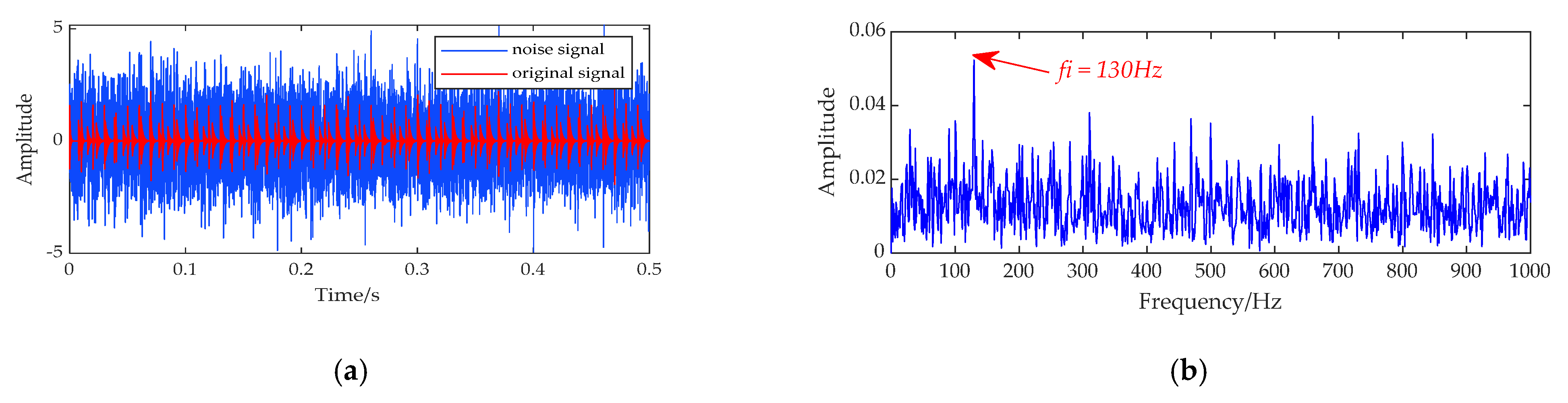
5.1. Simulation Signal

To construct the simulation signal of the bearing outer ring fault:

$$y_1(t)=y_0{e}^{-2\pi \varsigma f_{n}t}\sin 2\pi f_n\sqrt{1-{\varsigma }^2}t$$

(32)

where $y_0=2$, $\varsigma =0.1$ is the damping coefficient, $f_n=3000Hz$ is the natural frequency, and $f_o=100Hz$ is the fault character frequency.

To construct the simulation signal of the bearing inner ring fault:

$$\{\begin{array}{l}{y}_2(t)={\displaystyle {\sum }_i{A}_{i}h(t-iT-{\tau }_i)}\\ A_i=1+A_0\cos (2\pi f_{r}t)\\ h(t)=\exp (-Ct)\sin (2\pi f_{n}t)\end{array}$$

(33)

where rotation frequency $f_r=30Hz$, attenuation index $C=700$, initial amplitude of the signal $A_0=0.3$, natural frequency $f_n=3000Hz$, fault character frequency $f_i=130Hz$.

If signal $y_1(t)$ and $y_2(t)$ are superimposed and noise $n(t)$ with SNR = −5 is added, then the simulated composite fault signal is: $y(t)=y_1(t)+y_2(t)+n(t)$.

The sampling frequency was set as $20KHz$, and the number of sampling points N = 10,000. Figure 5 shows the time domain waveform (a) and envelope spectrum (b) of the simulation signal. From Figure 5b, only 1 time of the characteristic frequency of the inner ring fault can be seen, and it is impossible to determine whether the bearing is faulty.

CLNGO-FMD was used to decompose the signal. The optimal parameters of FMD were L = 82 and n = 3. The convergence curve of SPC (Figure 6a) and the time domain (Figure 6b) of each mode showed that the signal was decomposed into three layers.

The kurtosis values of each component were calculated as 3.4618, 3.0763, 3.0787, and the mode 1 with the largest value was selected for CLNGO-MNAD analysis. For outer ring feature extraction, FCF = 100 Hz, the convergence curve of the SPC value is shown in Figure 7a, the time-domain waveform in Figure 7b, the envelope spectrum in Figure 7c, and the optimal parameters were L = 660, $\rho =0.84$. For inner ring feature extraction, FCF = 130 Hz, the SPC iteration curve is shown in Figure 8a, the time domain in Figure 8b and the envelope spectrum in Figure 8c, and the optimal parameters were L = 800, $\rho =0.9$, from which the fault feature frequency and its frequency doubling component can be clearly seen. Furthermore, their values were close to the theoretical values.

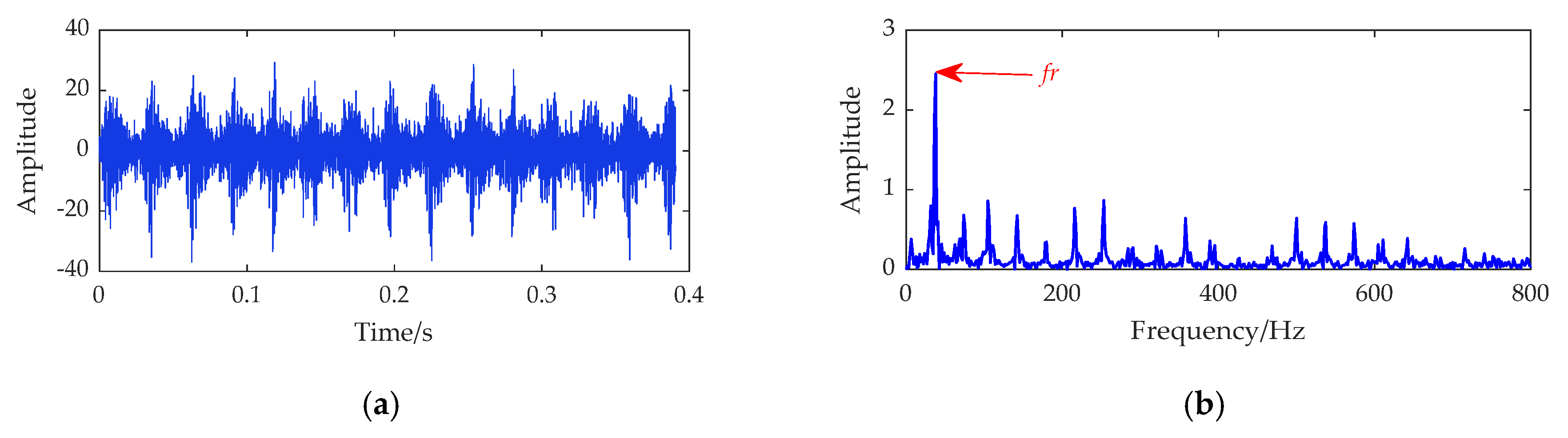
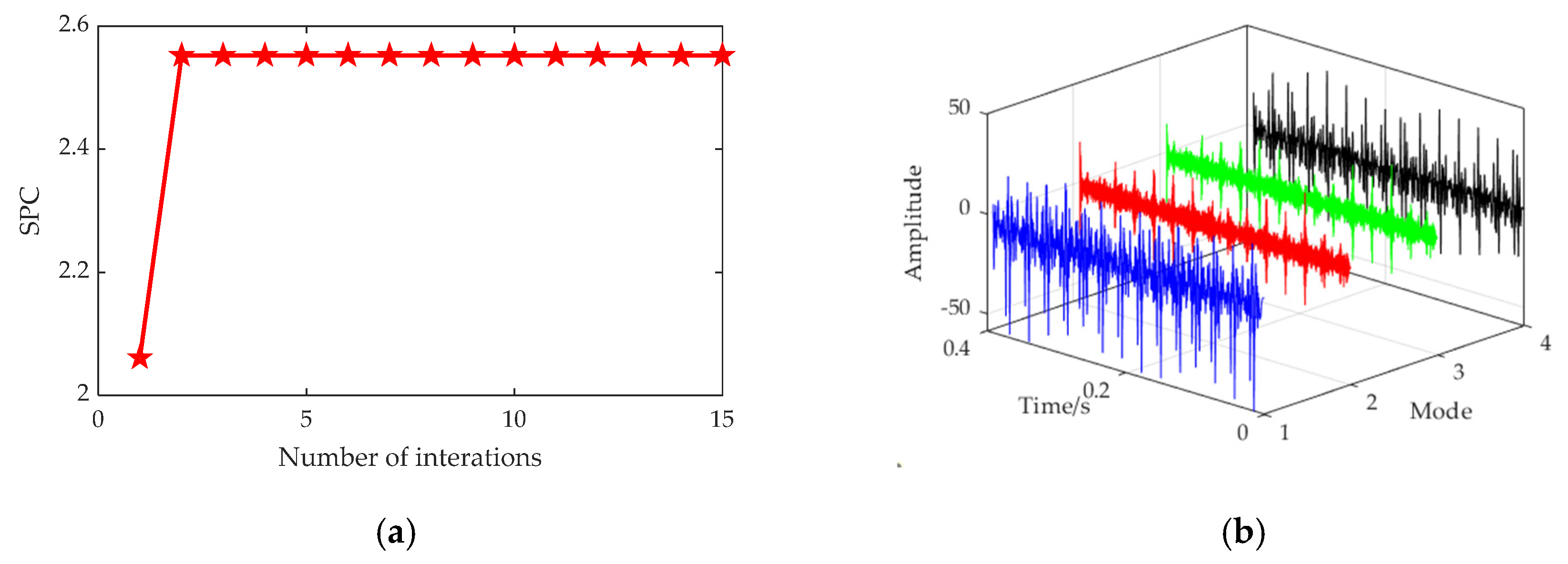
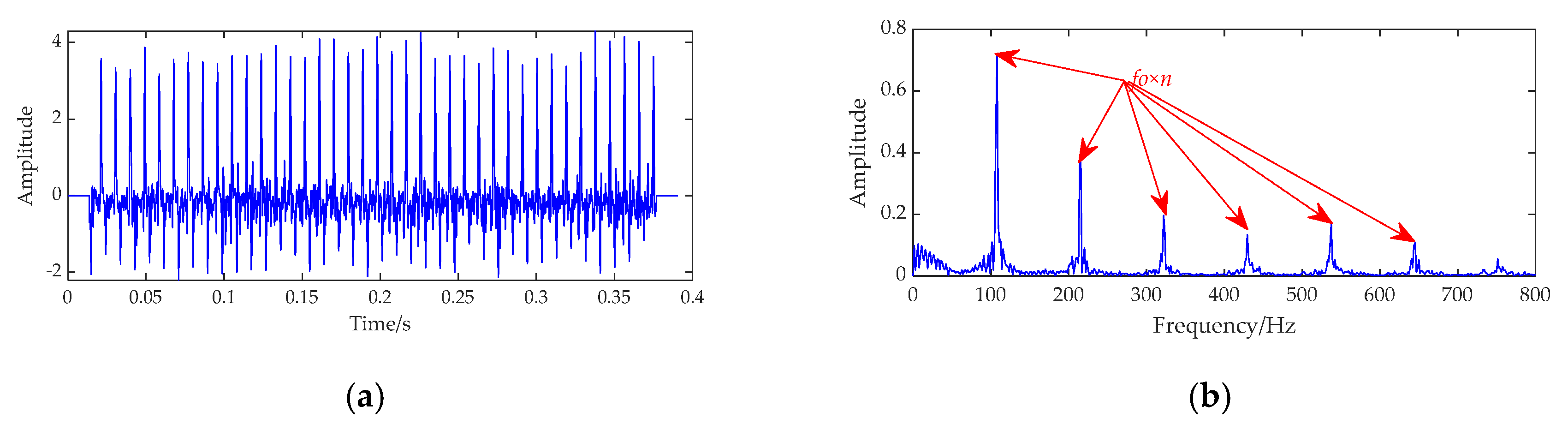
5.2. Experimental Analysis

Data from Xi‘an Jiaotong University’s bearing accelerated life test bench were selected for analysis [32].

Table 4. LDK UER204 model bearing parameters.

Middle Diameter of Bearing	Contact Angle	Diameter of Ball Bearing	Number of Ball Bearings
D = 34.55 mm	$\alpha =0°$	d = 7.92 mm	z = 8

shows the bearing parameters (sampling frequency $f=\mathrm{25,600}\mathrm{Hz}$).

The calculation formula of the bearing fault characteristic frequency is as follows:

$$f_i=\frac{n}{60}(1+\frac{d}{D}\cos \alpha )\frac{z}{2}$$

(34)

$$f_o=\frac{n}{60}(1-\frac{d}{D}\cos \alpha )\frac{z}{2}$$

(35)

where $n$ is rotation speed.

5.2.1. Inner Ring Fault

The later data of Bearing 2_1 were selected, and the bearing speed was $n=2250r/\min$. The frequency of $f_i=184\mathrm{Hz}$ was calculated using Equation (34), and the sampling number was set to 10,000. Figure 9 is the time domain diagram (a) and envelope spectrum (b) of the signal. In Figure 9b, we can only see the signal conversion frequency $f_r$, and cannot observe the bearing fault characteristic frequency and other frequency doubling components. Therefore, it is not possible to directly analyze whether the bearing is faulty from the envelope diagram of the original signal, and further analysis of the signal is needed.

CLNGO-FMD was used to decompose the signal. The optimal parameters of FMD were L = 69 and n = 4. The convergence curve of SPC (Figure 10a) and the time-domain (Figure 10b) of each mode showed that the signal was decomposed into three layers.

The calculated kurtosis of each mode was 5.2620, 8.4633, 9.4400, and 5.2869. The two modes 2 and 3 with the largest values were selected for reconstruction and secondary noise reduction and envelope analysis using CLNGO-MNAD. The optimal parameters of MNAD were L = 720, $\rho =0.85$ The result is shown in Figure 11 using CLNGO-MNAD. The fault characteristic frequency was 183.6 Hz and its multiple (Figure 11c), which proved that the inner ring of the bearing was damaged. The kurtosis values of modes 1 and 4 were both greater than 3 and had obvious periodic impact, which were reconstructed and analyzed using CLNGO-MNAD. The result is shown in Figure 12, which proves that this method can be used for bearing inner ring fault diagnosis.

5.2.2. Outer Ring Fault

The early data of Bearing 1_2 were selected, and the bearing speed s $n=2100r/\min$. The frequency of $f_o=107.9\mathrm{Hz}$ was calculated using Equation (34), and the fault feature extraction method for the inner ring and outer ring was the same. The results are presented in this section. The optimal parameters for the CLNGO-FMD were L = 50, n = 5. The optimal parameters of the CLNGO-FMD were L = 800, $\rho =0.88$. Figure 13 shows the time-domain waveform and envelope spectrum of the outer ring fault signal, and Figure 14 shows the decomposition results using CLNGO-FMD. The calculated kurtosis values of each mode were 3.8346, 3.0806, 4.7528, 3.3982, and 3.4149, and the signal was reconstructed and processed further. Figure 15 shows the result by CLNGO-MNAD.

5.2.3. Composite Fault (Inner Ring and Outer Ring Damage)

Bearing 1_5 late fault data were selected, and the bearing speed was, $f_o=107.9\mathrm{Hz}$ and $f_i=172.1\mathrm{Hz}$ were calculated using Equations (34) and (35), The feature extraction process was the same as that in Section 5.2, and only the results are presented in this section, The optimal parameters of FMD were L = 4, n = 5. The optimal parameters of MNAD when extracting outer ring features were L = 730, $\rho =0.16$, Figure 16 shows the time-domain waveform and envelope spectrum of the composite fault signal. Figure 17 shows the result of the decomposition using CLNGO-FMD.

By observing mode 1 in Figure 17, the impact component was obvious and periodically distributed. The envelope analysis of mode 1 is shown in Figure 18, $f_o$ and its frequency double can be clearly seen, which proves that CLNGO-FMD can adaptively realize the separation of different faults. However, CLNGO-FMD cannot realize the feature extraction of the inner circle, which still needs further analysis. The calculated kurtosis of each mode is 2.8012, 4.2408, 3.0139, 3.2462, 4.4881, and the signal was reconstructed and processed further. Figure 19 shows the results processed using CLNGO-MNAD.

In Figure 19b, the characteristic frequency of outer ring faults appears, indicating that FMD still has shortcomings in separating different faults and needs further improvement.

5.2.4. Comparison and Analysis

The EMD-MNAD, VMD-MNAD, FMD-MCKD and FMD-MOMEDA methods were selected for comparison. This section only analyzes the outer ring fault. Parameter settings of the algorithm are shown in

Table 5. Parameter settings for different algorithms.

Algorithm	MNAD	VMD	FMD	MCKD	MOMEDA
Parameter Settings	L = 40 ρ = 5	K = 6 α = 1500	L = 40 N = 5	L = 600 T = 230	L = 600 T =230

, and the results are shown in Figure 20. It is obvious that the proposed method is superior to other methods in feature extraction.

6. Conclusions

To solve the problem that it is difficult to extract features from rolling bearing composite faults, this paper proposes a feature extraction method based on the CLNGO algorithm to optimize FMD and MNAD, and verifies its effectiveness through simulation signals and experimental data. The main contributions of this paper are as follows: (1) The NGO algorithm is improved by introducing chaotic mapping and leader mutation selection strategy, and it is verified that CLNGO is superior to NGO in both convergence speed and convergence accuracy. (2) The CLNGO algorithm is used to select key parameters in FMD and MNAD, which makes it self-adaptive. Compared with VMD and EMD, FMD, this method can realize better separation of fault information and noise, and the proposed method is superior to MOMEDA and MCKD combined with envelope analysis in terms of fault feature extraction. (3) A new indicator SPC representing signal sparsity features is proposed as the fitness function of CLNGO, and the optimal parameters of FMD and MNAD are adaptively selected. The proposed method realizes the second denoising of signals and the separation of different fault information in composite faults, which provides a new method for rolling bearing fault diagnosis.

References

1. Berredjem, T.; Benidir, M. Bearing faults diagnosis using fuzzy expert system relying on an Improved Range Overlaps and Similarity method. Expert Syst. Appl. 2018, 108, 134–142. [Google Scholar] [CrossRef]
2. Qian, C.H.; Jiang, Q.S.; Shen, Y.; Huo, C.; Zhang, Q. An intelligent fault diagnosis method for rolling bearings based on feature transfer with improved DenseNet and joint distribution adaptation. Meas. Sci. Technol. 2022, 33, 025101. [Google Scholar] [CrossRef]
3. Song, X.J.; Zhao, W.X. A Review of Rolling Bearings Fault Diagnosis Approaches Using AC Motor Signature Analysis. Proc. CSEE 2021, 42, 1582–1596. [Google Scholar] [CrossRef]
4. Zhang, Y.H.; Zhou, T.T.; Subburam, V. Fault diagnosis of rotating machinery based on recurrent neural networks. Measurement 2021, 171, 108774. [Google Scholar] [CrossRef]
5. Zhang, F.; Sun, W.L.; Wang, H.; Xu, T. Fault Diagnosis of a Wind Turbine Gearbox Based on Improved Variational Mode Algorithm and Information Entropy. Entropy 2021, 23, 794. [Google Scholar] [CrossRef]
6. Cai, J.H.; Hu, W.W.; Wang, X.C. Fault diagnosis of rolling bearing based on EMD-ICA de-noising. J. Mach. Des. 2015, 32, 17–23. [Google Scholar] [CrossRef]
7. Bai, L.; Xi, W. Early Fault Diagnosis of Rolling Bearing Based Empirical Wavelet Transform and Spectral Kurtosis. In Proceedings of the 2018 IEEE International Conference on Prognostics and Health Management (ICPHM), Seattle, WA, USA, 11–13 June 2018; pp. 1–6. [Google Scholar]
8. Gundewar, S.K.; Kane, P.V. Bearing fault diagnosis using time segmented Fourier synchrosqueezed transform images and convolution neural network. Measurement 2022, 203, 111855. [Google Scholar] [CrossRef]
9. Dragomiretskiy, K.; Zosso, D. Variational Mode Decomposition. IEEE Trans. Signal Process. 2014, 62, 531–544. [Google Scholar] [CrossRef]
10. Ye, M.; Yan, X.; Jia, M. Rolling Bearing Fault Diagnosis Based on VMD-MPE and PSO-SVM. Entropy 2021, 23, 762. [Google Scholar] [CrossRef]
11. Cheng, J.; Yang, Y.; Shao, H.; Pan, H.; Zheng, J.; Cheng, J. Enhanced periodic mode decomposition and its application to composite fault diagnosis of rolling bearings. ISA Trans. 2021, 125, 474–491. [Google Scholar] [CrossRef]
12. Li, T.Y.; Kou, Z.M.; Wu, J.; Yang, F. Application of Adaptive MOMEDA with Iterative Autocorrelation to Enhance Weak Features of Hoist Bearings. Entropy 2021, 23, 789. [Google Scholar] [CrossRef] [PubMed]
13. Zeng, M.; Chen, Z. SOSO Boosting of the K-SVD Denoising Algorithm for Enhancing Fault-Induced Impulse Responses of Rolling Element Bearings. IEEE Trans. Ind. Electron. 2020, 67, 1282–1292. [Google Scholar] [CrossRef]
14. Miao, Y.H.; Zhang, B.; Li, C.; Lin, J.; Zhang, D. Feature Mode Decomposition: New Decomposition Theory for Rotating Machinery Fault Diagnosis. IEEE Trans. Ind. Electron. 2022, 70, 1949–1960. [Google Scholar] [CrossRef]
15. Wiggins, R.A. Minimum entropy deconvolution. Geoexploration 1978, 16, 21–35. [Google Scholar] [CrossRef]
16. Sun, Y.H.; Yu, J.B. Adaptive Sparse Representation-Based Minimum Entropy Deconvolution for Bearing Fault Detection. IEEE Trans. Instrum. Meas. 2022, 71, 3513010. [Google Scholar] [CrossRef]
17. Sun, H.; Liang, F.W.; Liu, Y.; Liu, K.; Wang, Z.; Zhang, T. Application of a Novel Improved Adaptive CYCBD Method in Gearbox Compound Fault Diagnosis. IEEE Access 2021, 9, 133835–133848. [Google Scholar] [CrossRef]
18. Mcdonald, G.L.; Zhao, Q.; Zuo, M.J. Maximum correlated kurtosis deconvolution and application on gear tooth chip fault detection. Mech. Syst. Signal Process. 2012, 33, 237–255. [Google Scholar] [CrossRef]
19. Fang, B.; Hu, J.; Yang, C.; Cao, Y.; Jia, M. A blind deconvolution algorithm based on backward automatic differentiation and its application to rolling bearing fault diagnosis. Meas. Sci. Technol. 2022, 33, 025009. [Google Scholar] [CrossRef]
20. Mirjalili, S.; Lewis, A. The Whale Optimization Algorithm. Adv. Eng. Softw. 2016, 95, 51–67. [Google Scholar] [CrossRef]
21. Mirjalili, S.; Lewis, A. Grey Wolf Optimizer. Adv. Eng. Softw. 2013, 69, 46–61. [Google Scholar] [CrossRef] [Green Version]
22. Hashim, F.A.; Houssein, E.H.; Hussain, K.; Mabrouk, M.S.; Al-Atabany, W. Honey Badger Algorithm: New Metaheuristic Algorithm for Solving Optimization Problems. Math. Comput. Simul. 2021, 192, 84–110. [Google Scholar] [CrossRef]
23. Heidari, A.A.; Faris, H.; Aljarah, I.; Mafarja, M.; Chen, H. Harris hawks optimization: Algorithm and applications. Future Gener. Comput. Syst. 2019, 97, 849–872. [Google Scholar] [CrossRef]
24. Dehghani, M.; Hubalovsky, S.; Trojovsky, P. Northern Goshawk Optimization: A New Swarm-Based Algorithm for Solving Optimization Problems. IEEE Access 2021, 9, 162059–162080. [Google Scholar] [CrossRef]
25. Ma, L.L.; Jiang, H.; Ma, T.; Zhang, X.; Shen, Y.; Xia, L. Fault Prediction of Rolling Element Bearings Using the Optimized MCKD–LSTM Model. Machines 2022, 10, 342. [Google Scholar] [CrossRef]
26. Wang, B.; Lei, Y.G.; Li, N. A Hybrid Prognostics Approach for Estimating Remaining Useful Life of Rolling Element Bearings. J. Eng. 2020, 69, 401–412. [Google Scholar] [CrossRef]
27. Wang, R.X.; Jiang, H.K.; Zhu, K.; Wangm, Y.; Liu, C. A deep feature enhanced reinforcement learning method for rolling bearing fault diagnosis. Adv. Eng. Inform. 2022, 54, 101750. [Google Scholar] [CrossRef]
28. Tang, J.H.; Wu, J.M.; Hu, B.; Liu, J. Towards a fault diagnosis method for rolling bearing with Bi-directional deep belief network. Appl. Acoust. 2022, 192, 108727. [Google Scholar] [CrossRef]
29. Li, J.; Liu, Y.H.; Li, Q.J. Intelligent fault diagnosis of rolling bearings under imbalanced data conditions using attention-based deep learning method. Measurement 2022, 189, 110500. [Google Scholar] [CrossRef]
30. Li, Y.F.; Han, T. Deep Learning Based Industrial Equipment Prognostics and Health Management: A Review. J. Vib. Meas. Diagn. 2022, 42, 835–847+1029. [Google Scholar] [CrossRef]
31. Miao, Y.H.; Wang, J.J.; Zhang, B.Y.; Li, H. Practical framework of Gini index in the application of machinery fault feature extraction. Mech. Syst. Signal Process. 2021, 165, 108333. [Google Scholar] [CrossRef]
32. Lei, Y.G.; Han, T.Y.; Wang, B.; Li, N.; Yan, T.; Yang, J. XJTU-SY Rolling Element Bearing Accelerated Life Test Datasets: A Tutorial. J. Mech. Eng. 2019, 55, 1–6. [Google Scholar] [CrossRef]
Figure 1. Flowchart of CLNGO optimizing FMD and MNAD.
Processes 10 02532 g001
Figure 2. Convergence curve of the high-dimensional single objective function. (a) The convergence curve of function f1. (b) The convergence curve of function f2. (c) The convergence curve of function f3. (d) The convergence curve of function f4.
Processes 10 02532 g002
Figure 3. Convergence curve of the high-dimensional multi-objective function. (a) The convergence curve of function f5. (b) The convergence curve of function f6. (c) The convergence curve of function f7. (d) The convergence curve of function f8.
Processes 10 02532 g003aProcesses 10 02532 g003b
Figure 4. Convergence curve of the low-dimensional test functions. (a) The convergence curve of function f9. (b) The convergence curve of function f10. (c) The convergence curve of function f11. (d) The convergence curve of function f12.
Processes 10 02532 g004
Figure 5. Time-domain waveforms (a) and envelope spectrum (b) of simulation signal. (a) Time-domain waveform. (b) Envelope spectrum.
Processes 10 02532 g005
Figure 6. Simulation signal is decomposed by CLNGO-FMD. (a) Convergence curve of SPC. (b) Time-domain waveform.
Processes 10 02532 g006
Figure 7. Outer ring fault feature extraction using CLNGO-MNAD. (a) Convergence curve of SPC. (b) Time-domain waveform. (c) Envelope spectrum.
Processes 10 02532 g007
Figure 8. Inner ring fault feature extraction using CLNGO-MNAD. (a) Convergence curve of SPC. (b) Time-domain waveform. (c) Envelope spectrum.
Processes 10 02532 g008
Figure 9. Time-domain waveforms (a) and envelope spectrum (b) of inner ring fault signal. (a) Time-domain waveform. (b) Envelope spectrum.
Processes 10 02532 g009
Figure 10. Inner ring fault signal is decomposed by CLNGO-FMD. (a) Convergence curve of SPC. (b) Time-domain waveform.
Processes 10 02532 g010
Figure 11. The results for modes 2 and 3 are processed by CLNGO-MNAD. (a) Convergence curve of SPC. (b) Time-domain waveform. (c) Envelope spectrum.
Processes 10 02532 g011
Figure 12. The results for modes 1 and 4 are processed by CLNGO-MNAD.
Processes 10 02532 g012
Figure 13. Outer ring fault signal. (a) Time-domain waveform. (b) Envelope spectrum.
Processes 10 02532 g013
Figure 14. Decomposition results of outer fault signals using CLNGO-FMD.
Processes 10 02532 g014
Figure 15. Outer ring fault signal. (a) Time-domain waveform using CLNGO-MNAD. (b) Envelope spectrum of using CLNGO-MNAD.
Processes 10 02532 g015
Figure 16. Composite fault signal. (a) Time-domain waveform. (b) Envelope spectrum.
Processes 10 02532 g016
Figure 17. Decomposition results of composite fault signals using CLNGO-FMD.
Processes 10 02532 g017
Figure 18. Envelope spectrum of mode 1.
Processes 10 02532 g018
Figure 19. Feature extraction of inner ring in composite fault signal. (a) Time-domain waveform using CLNGO-MNAD. (b) Envelope spectrum using CLNGO-MNAD.
Processes 10 02532 g019
Figure 20. Comparing the results of different methods (outer fault signals).
Processes 10 02532 g020