

Causal Plot: Causal-Based Fault Diagnosis Method Based on Causal Analysis


Abstract
1. Introduction
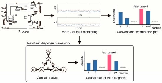
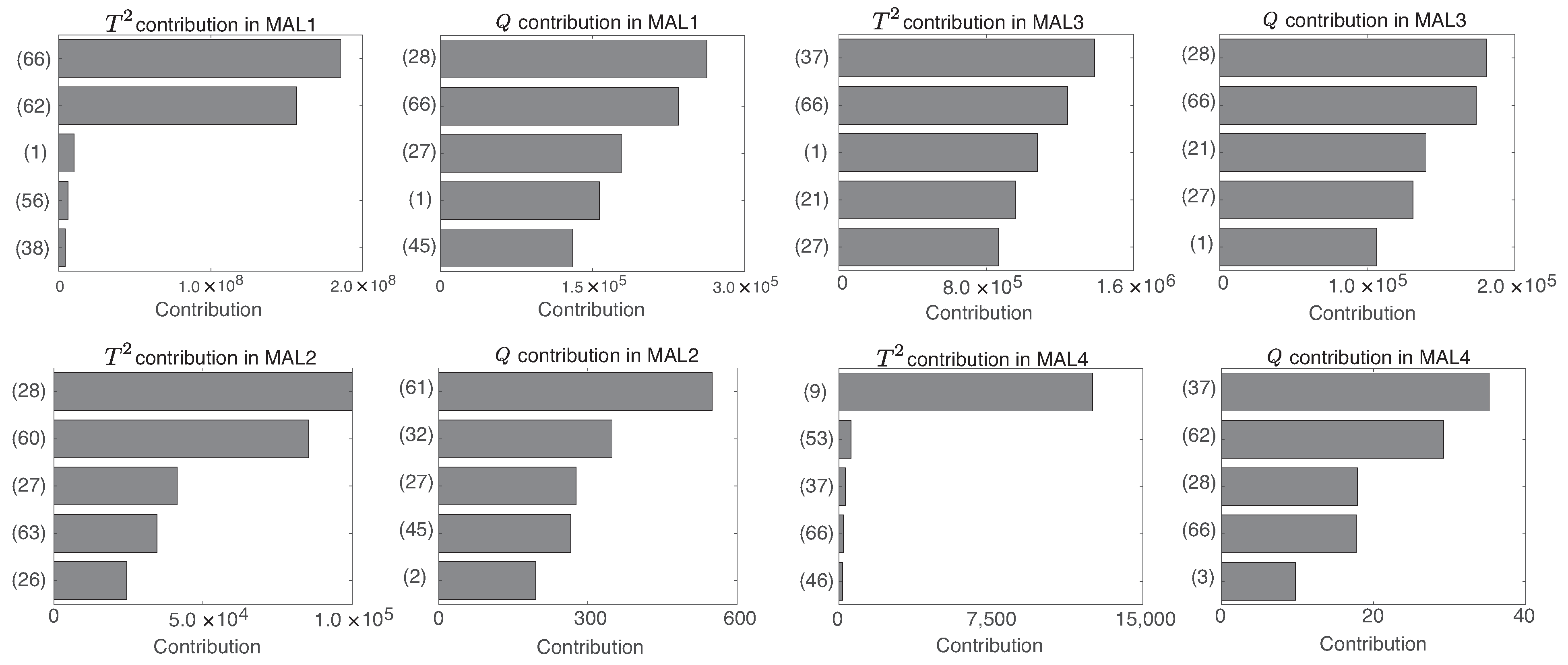
2. Contribution Plot
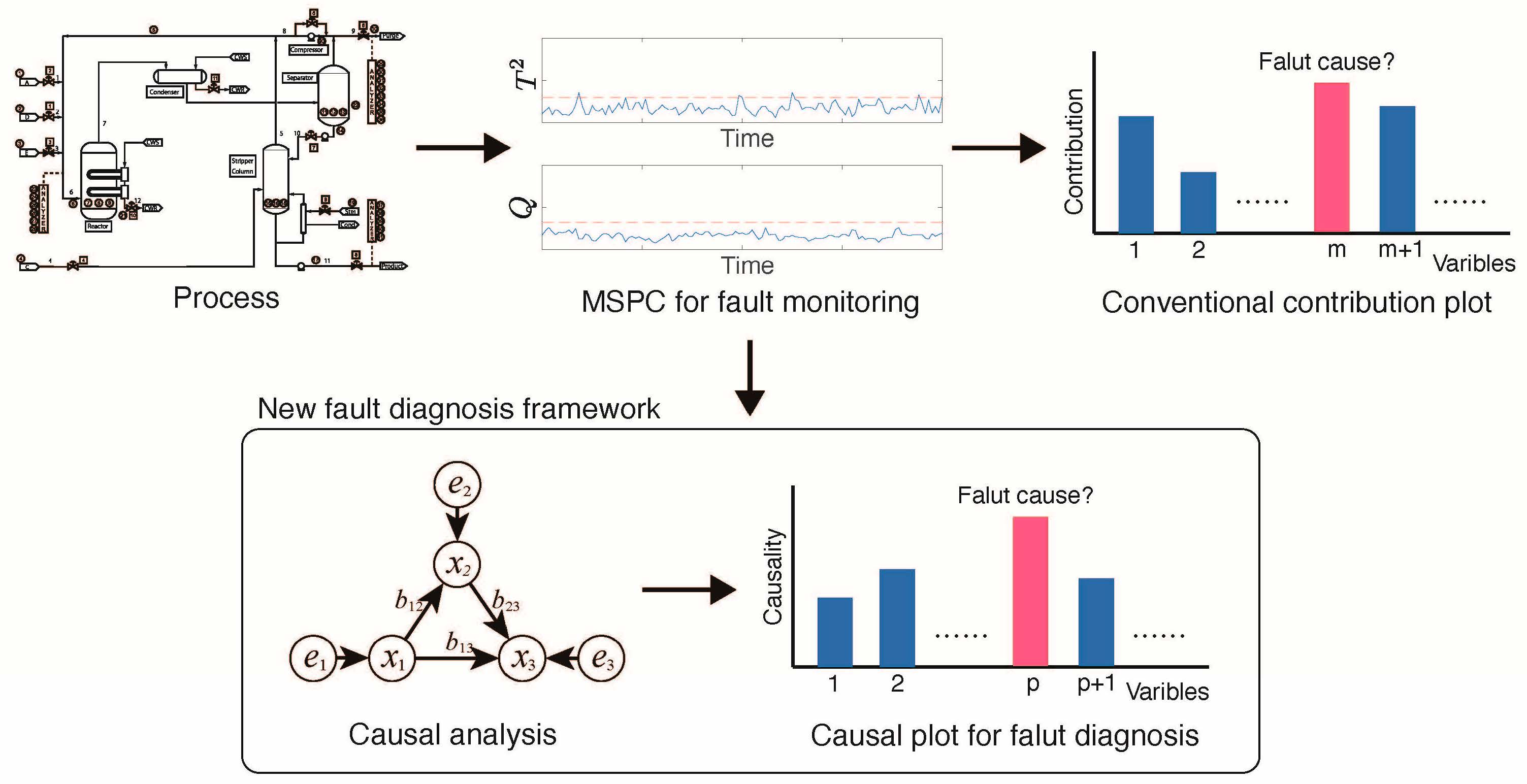
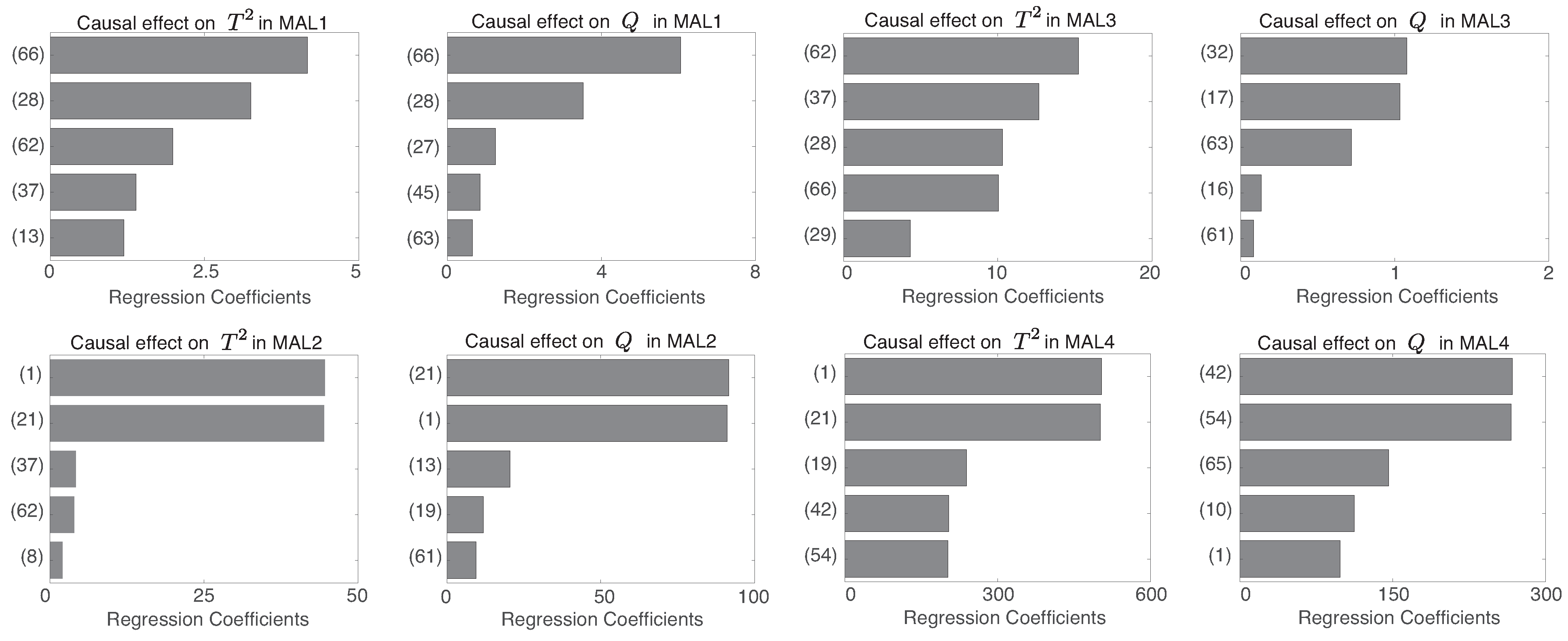
3. Causal Plot
- Generate the ith input vector when a fault is detected between times s and .
- Merge into one matrix: .
- Apply to LiNGAM and calculate the LiNGAM coefficient matrix .
- Extract the th column vector of as the causal plot.
4. Case Study
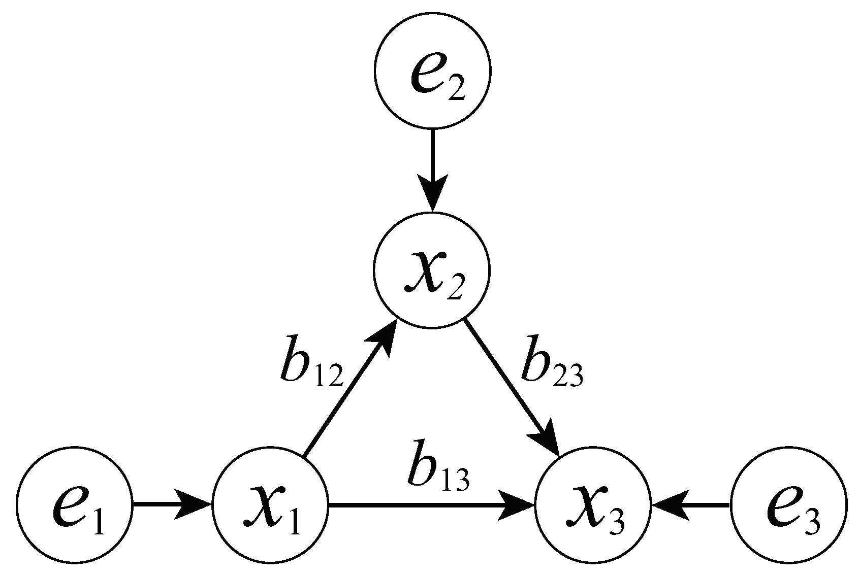
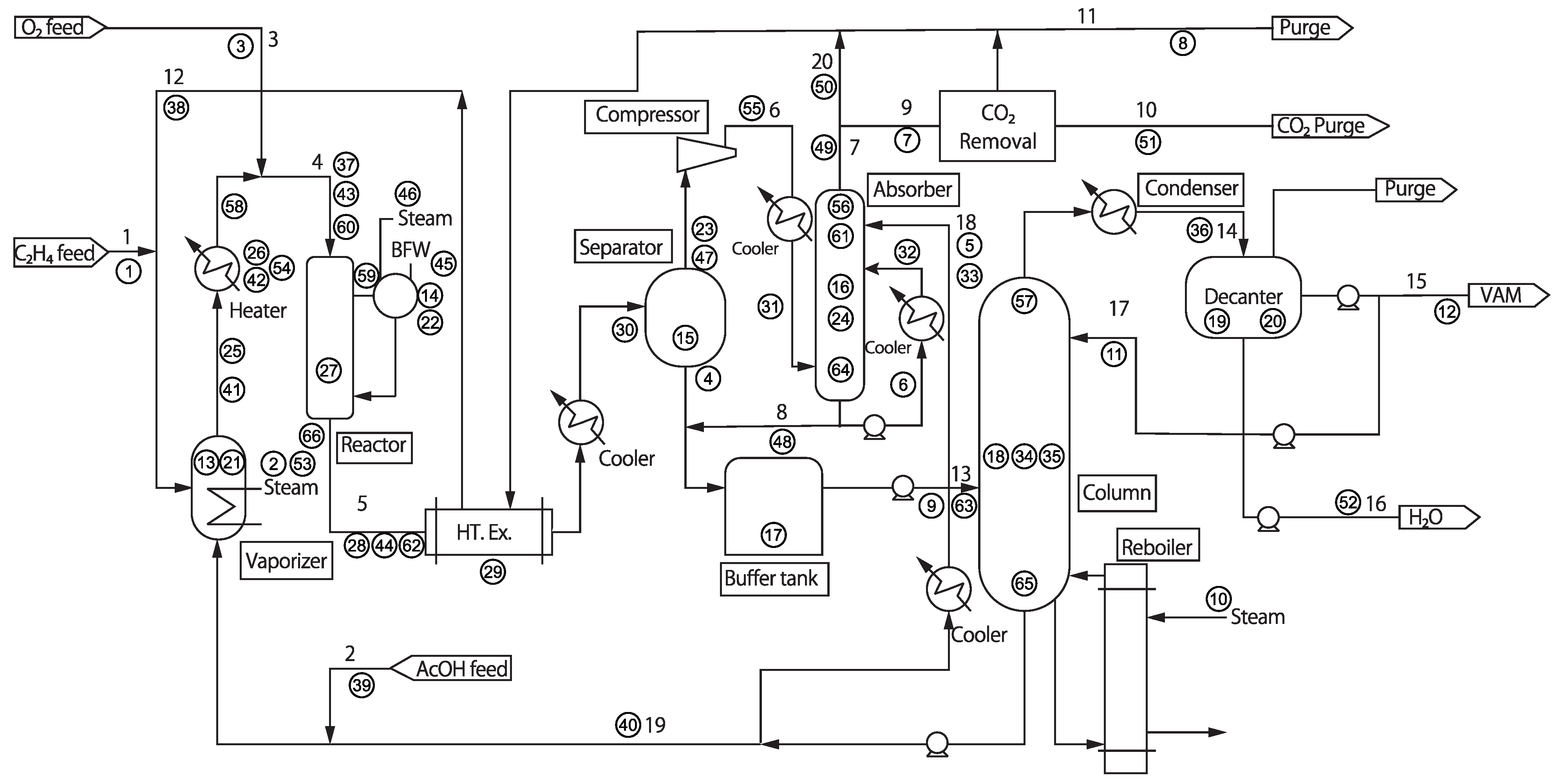
4.1. VAM Process
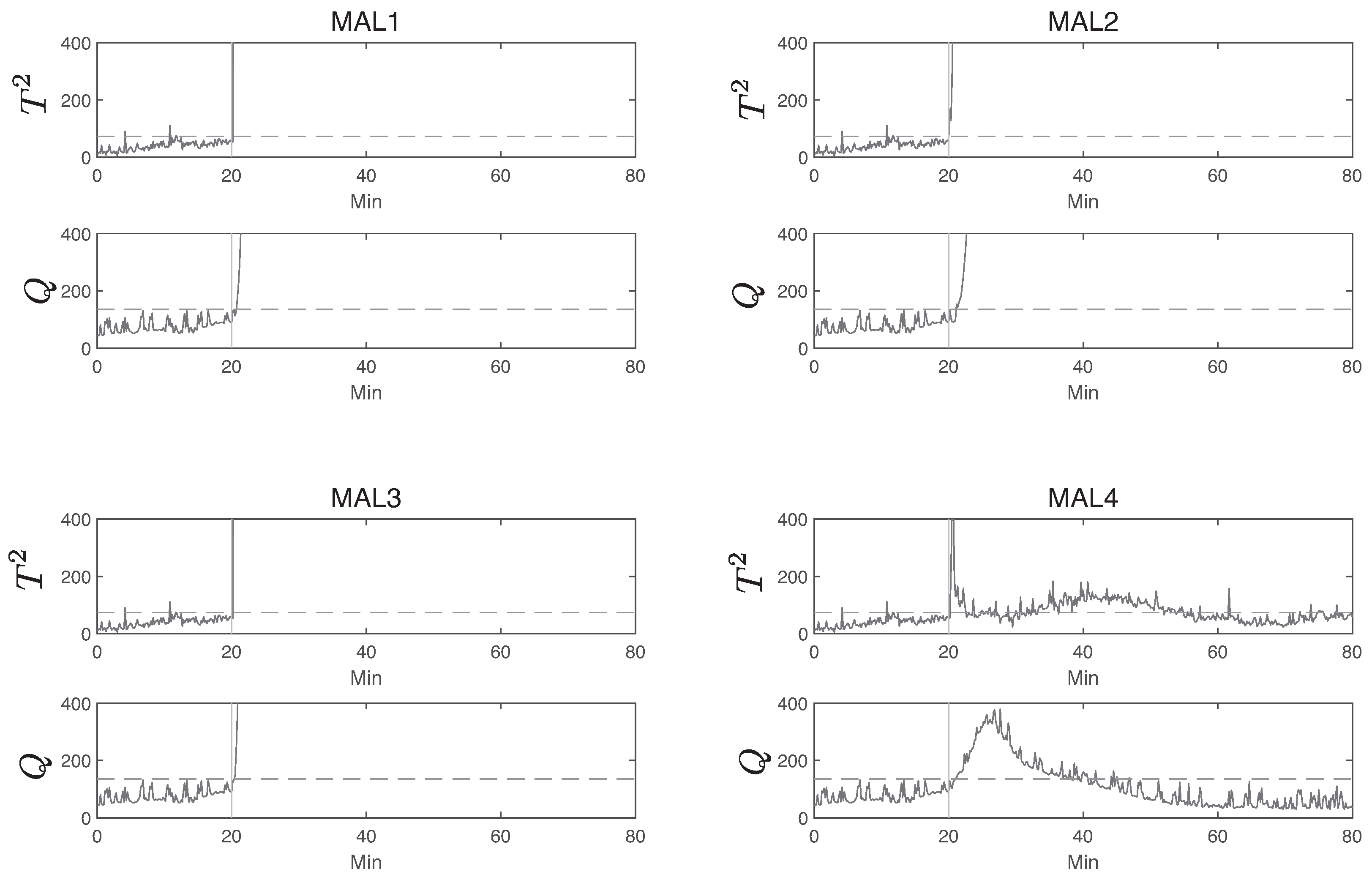
4.2. Fault Detection
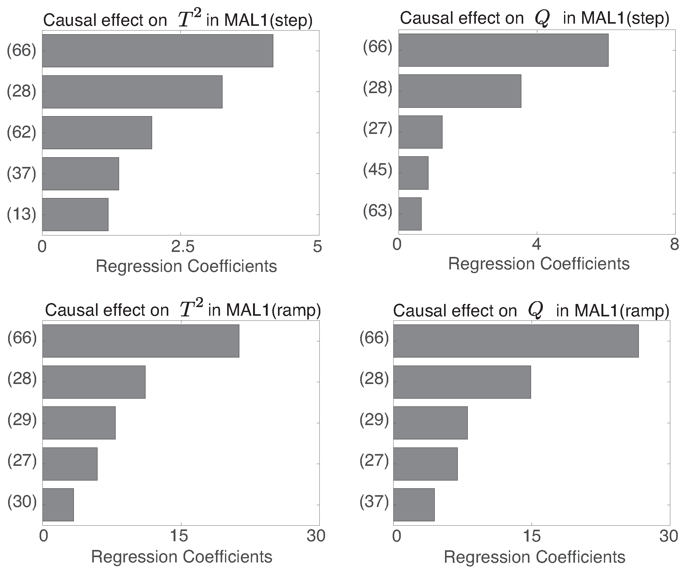
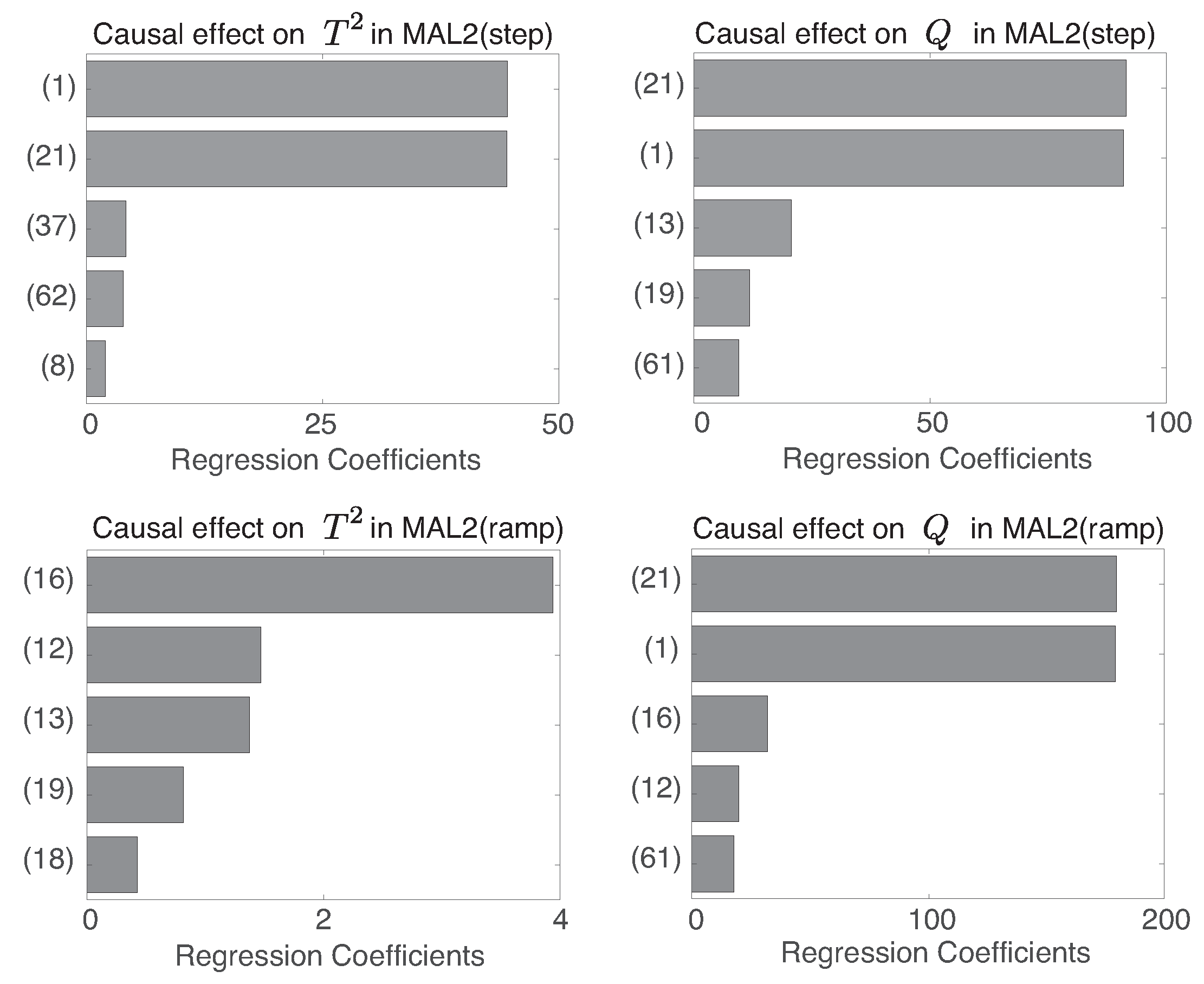
4.3. Fault Diagnosis
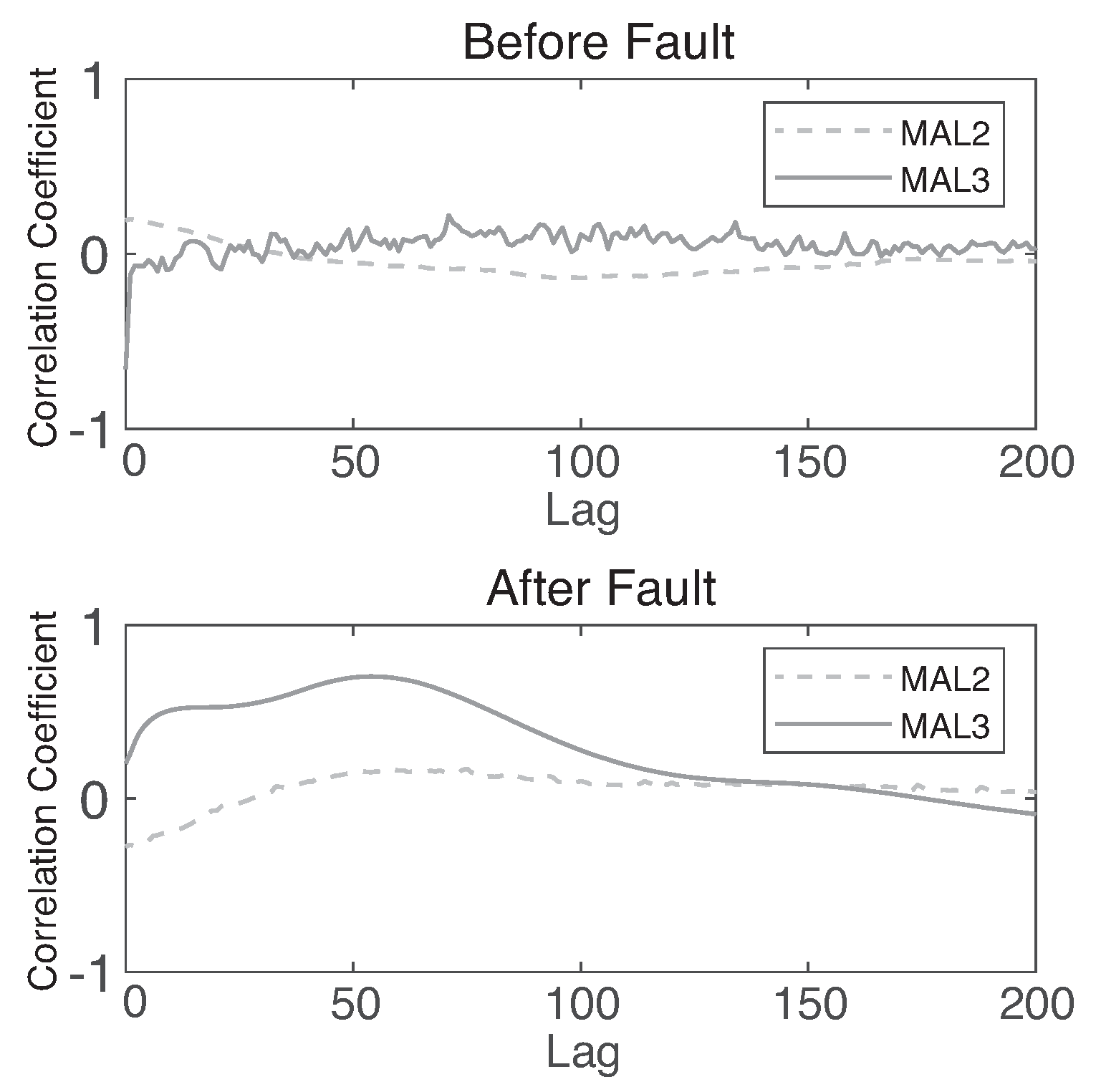
4.4. Discussion
5. Conclusions
Supplementary Materials
Author Contributions
Funding
Data Availability Statement
Conflicts of Interest
References
- Jiang, Y.; Yin, S.; Dong, J.; Kaynak, O. A Review on Soft Sensors for Monitoring, Control, and Optimization of Industrial Processes. IEEE Sens. J. 2021, 21, 12868–12881. [Google Scholar] [CrossRef]
- Zhang, X.; Wang, H.; Stojanovic, V.; Cheng, P.; He, S.; Luan, X.; Liu, F. Asynchronous Fault Detection for Interval Type-2 Fuzzy Nonhomogeneous Higher Level Markov Jump Systems With Uncertain Transition Probabilities. IEEE Trans. Fuzzy Syst. 2022, 30, 2487–2499. [Google Scholar] [CrossRef]
- Müller, R.; Oehm, L. Process Industries versus Discrete Processing: How System Characteristics Affect Operator Tasks. Cogn. Technol. Work 2019, 21, 337–356. [Google Scholar] [CrossRef]
- MacGregor, J.F.; Jaeckle, C.; Kiparissides, C.; Koutoudi, M. Process Monitoring and Diagnosis by Multiblock PLS Methods. AIChE J. 1994, 40, 826–838. [Google Scholar] [CrossRef]
- Koeman, M.; Engel, J.; Jansen, J.; Buydens, L. Critical comparison of methods for fault diagnosis in metabolomics data. Sci. Rep. 2019, 9, 1123. [Google Scholar] [CrossRef]
- Zhao, L.T.; Yang, T.; Yan, R.; Zhao, H.B. Anomaly detection of the blast furnace smelting process using an improved multivariate statistical process control model. Process Saf. Environ. Prot. 2022, 166, 617–627. [Google Scholar] [CrossRef]
- Yoon, S.; MacGregor, J.F. Statistical and Causal Model-Based Approaches to Fault Detection and Isolation. AIChE J. 2000, 46, 1813–1824. [Google Scholar] [CrossRef]
- Westerhuis, J.A.; Gurden, S.P.; Smilde, A.K. Generalized Contribution Plots in Multivariate Statistical Process Monitoring. Chemom. Intell. Lab. Syst. 2000, 51, 95–114. [Google Scholar] [CrossRef]
- Amin, M.T.; Imtiaz, S.; Khan, F. Process System Fault Detection and Diagnosis Using a Hybrid Technique. Chem. Eng. Sci. 2018, 189, 191–211. [Google Scholar] [CrossRef]
- Yu, H.; Khan, F.; Garaniya, V. Modified Independent Component Analysis and Bayesian Network-Based Two-Stage Fault Diagnosis of Process Operations. Ind. Eng. Chem. Res. 2015, 54, 2724–2742. [Google Scholar] [CrossRef]
- Chen, H.S.; Yan, Z.; Yao, Y.; Huang, T.B.; Wong, Y.S. Systematic Procedure for Granger-Causality-Based Root Cause Diagnosis of Chemical Process Faults. Ind. Eng. Chem. Res. 2018, 57, 9500–9512. [Google Scholar] [CrossRef]
- Yuan, T.; Qin, S.J. Root cause diagnosis of plant-wide oscillations using Granger causality. J. Process Control 2014, 24, 450–459. [Google Scholar] [CrossRef]
- Liu, Y.; Chen, H.S.; Wu, H.; Dai, Y.; Yao, Y.; Yan, Z. Simplified Granger causality map for data-driven root cause diagnosis of process disturbances. J. Process Control 2020, 95, 45–54. [Google Scholar] [CrossRef]
- Granger, C.W.J. Investigating Causal Relations by Econometric Models and Cross-spectral Methods. Econometrica 1969, 37, 424–438. [Google Scholar] [CrossRef]
- Shimizu, S.; Hoyer, P.O.; Hyvärinen, A.; Kerminen, A. A Linear Non-Gaussian Acyclic Model for Causal Discovery. J. Mach. Learn. Res. 2006, 7, 2003–2030. [Google Scholar]
- Lai, P.C.; Bessler, D.A. Price Discovery Between Carbonated Soft Drink Manufacturers and Retailers: A Disaggregate Analysis with Pc and Lingam Algorithms. J. Appl. Econ. 2015, 18, 173–197. [Google Scholar] [CrossRef]
- Luyben, M.L.; Tyréus, B.D. An Industrial Design/Control Study for the Vinyl Acetate Monomer Process. Comput. Chem. Eng. 1998, 22, 867–877. [Google Scholar] [CrossRef]
- Machida, Y.; Ootakara, S.; Seki, H.; Hashimoto, Y.; Kano, M.; Miyake, Y.; Anzai, N.; Sawai, M.; Katsuno, T.; Omata, T. Vinyl Acetate Monomer (VAM) Plant Model: A New Benchmark Problem for Control and Operation Study. IFAC-PapersOnLine 2016, 49, 533–538. [Google Scholar] [CrossRef]
- Uchida, Y.; Fujiwara, K.; Saito, T.; Osaka, T. Process Fault Diagnosis Method Based on MSPC and LiNGAM and its Application to Tennessee Eastman Process. IFAC-PapersOnLine 2022, 55, 384–389. [Google Scholar] [CrossRef]
- Jackson, J.E.; Mudholkar, G. Control Procedures for Residuals Associated With Principal Component Analysis. Technometrics 1979, 21, 341–349. [Google Scholar] [CrossRef]
- Kaiser, H.F. The Application of Electronic Computers to Factor Analysis. Educ. Psychol. Meas. 1960, 20, 141–151. [Google Scholar] [CrossRef]
- Ji, C.; Sun, W. A Review on Data-Driven Process Monitoring Methods: Characterization and Mining of Industrial Data. Processes 2022, 10, 335. [Google Scholar] [CrossRef]
- Lee, J.M.; Yoo, C.; Choi, S.W.; Vanrolleghem, P.A.; Lee, I.B. Nonlinear process monitoring using kernel principal component analysis. Chem. Eng. Sci. 2004, 59, 223–234. [Google Scholar] [CrossRef]
- Kano, M.; Tanaka, S.; Hasebe, S.; Hashimoto, I.; Ohno, H. Monitoring independent components for fault detection. AIChE J. 2003, 49, 969–976. [Google Scholar] [CrossRef]
- Chen, Z.; Cao, Y.; Ding, S.X.; Zhang, K.; Koenings, T.; Peng, T.; Yang, C.; Gui, W. A Distributed Canonical Correlation Analysis-Based Fault Detection Method for Plant-Wide Process Monitoring. IEEE Trans. Industr. Inform. 2019, 15, 2710–2720. [Google Scholar] [CrossRef]
- Kano, M.; Ogawa, M. The state of the art in chemical process control in Japan: Good practice and questionnaire survey. J. Process Control 2010, 20, 969–982. [Google Scholar] [CrossRef]
- Nomikos, P. Detection and Diagnosis of Abnormal Batch Operations Based on Multi-Way Principal Component Analysis World Batch Forum, Toronto, May 1996. ISA Trans. 1996, 35, 259–266. [Google Scholar] [CrossRef]
- Uchida, T.; Fujiwara, K.; Nishioji, K.; Kobayashi, M.; Kano, M.; Seko, Y.; Yamaguchi, K.; Itoh, Y.; Kadotani, H. Medical checkup data analysis method based on LiNGAM and its application to nonalcoholic fatty liver disease. Artif. Intell. Med. 2022, 128, 102310. [Google Scholar] [CrossRef]
- Shimizu, S.; Inazumi, T.; Sogawa, Y.; Hyvärinen, A.; Kawahara, Y.; Washio, T.; Hoyer, P.O.; Bollen, K. DirectLiNGAM: A Direct Method for Learning a Linear Non-Gaussian Structural Equation Model. J. Mach. Learn. Res 2011, 12, 1225–1248. [Google Scholar]
- Berbache, S.; Harkat, M.F.; Kratz, F. Sensor fault detection and isolation techniques based on PCA. In Proceedings of the 2019 International Conference on Advanced Electrical Engineering (ICAEE), Algiers, Algeria, 19–21 November 2019. [Google Scholar]
- Kanse, L.; Schaaf, T. Recovery From Failures in the Chemical Process Industry. Int. J. Cogn. Ergon. 2001, 5, 199–211. [Google Scholar] [CrossRef]
- Reinartz, C.; Kulahci, M.; Ravn, O. An extended Tennessee Eastman simulation dataset for fault-detection and decision support systems. Comput. Chem. Eng. 2021, 149, 107281. [Google Scholar] [CrossRef]
- Shahbazinia, A.; Salehkaleybar, S.; Hashemi, M. ParaLiNGAM: Parallel Causal Structure Learning for Linear Non-Gaussian Acyclic Models. arXiv 2021, arXiv:2109.13993. [Google Scholar] [CrossRef]


| No. | Variables | No. | Variables |
|---|---|---|---|
| 1 | stream 1 flow | 34 | column temperature |
| 2 | vaporizer steam flow | 35 | column temperature (control) |
| 3 | stream 3 flow | 36 | stream 14 temperature |
| 4 | separator outflow | 37 | stream 4 molarity |
| 5 | stream 18 flow | 38 | stream 12 flow |
| 6 | absorber recycle flow | 39 | stream 2 flow |
| 7 | stream 9 flow | 40 | stream 19 flow |
| 8 | stream 11 flow | 41 | vaporizer outflow |
| 9 | stream 13 flow | 42 | heater steam flow |
| 10 | column steam flow | 43 | stream 4 flow |
| 11 | stream 17 flow | 44 | stream 5 flow |
| 12 | stream 15 flow | 45 | steam drum return flow |
| 13 | vaporizer level | 46 | steam drum inflow |
| 14 | steam drum level | 47 | separator gas outflow |
| 15 | separator level | 48 | stream 8 flow |
| 16 | absorber level | 49 | stream 7 flow |
| 17 | buffer tank level | 50 | stream 20 flow |
| 18 | column level | 51 | stream 10 flow |
| 19 | decanter sediment level | 52 | stream 16 flow |
| 20 | decanter non-sediment level | 53 | vaporizer steam pressure |
| 21 | vaporizer pressure | 54 | heater steam pressure |
| 22 | steam drum pressure | 55 | stream 6 pressure |
| 23 | separator outflow gas pressure | 56 | absober top pressure |
| 24 | column pressure | 57 | column top pressure |
| 25 | vaporizer outflow temperature | 58 | heater outflow temperature |
| 26 | heater temperature | 59 | reactor inflow steam temperature |
| 27 | reactor temperature | 60 | reactor inlet temperature |
| 28 | stream 5 temperature | 61 | absorber top temperature |
| 29 | temperature after heat exchange | 62 | stream 5 molarity |
| 30 | separator inflow temperature | 63 | stream 13 flow (control) |
| 31 | absorber inflow temperature from separator | 64 | absorber bottom pressure |
| 32 | absorber recycle temperature | 65 | column bottom pressure |
| 33 | absorber inflow temperature from column | 66 | reactor outlet temperature |
| No. | Description | Type |
|---|---|---|
| 1 | feed composition | step |
| 2 | AcOH feed composition | step |
| 3 | feed pressure | ramp |
| 4 | feed pressure | ramp |
| Method | Contribution Plot | Causal Plot | ||
|---|---|---|---|---|
| Statistic | ||||
| MAL1 | correct | correct | correct | correct |
| MAL2 | incorrect | incorrect | correct | correct |
| MAL3 | correct | correct | correct | incorrect |
| MAL4 | incorrect | correct | correct | correct |
Publisher’s Note: MDPI stays neutral with regard to jurisdictional claims in published maps and institutional affiliations. |
© 2022 by the authors. Licensee MDPI, Basel, Switzerland. This article is an open access article distributed under the terms and conditions of the Creative Commons Attribution (CC BY) license (https://creativecommons.org/licenses/by/4.0/).
Share and Cite
Uchida, Y.; Fujiwara, K.; Saito, T.; Osaka, T. Causal Plot: Causal-Based Fault Diagnosis Method Based on Causal Analysis. Processes 2022, 10, 2269. https://doi.org/10.3390/pr10112269
Uchida Y, Fujiwara K, Saito T, Osaka T. Causal Plot: Causal-Based Fault Diagnosis Method Based on Causal Analysis. Processes. 2022; 10(11):2269. https://doi.org/10.3390/pr10112269
Chicago/Turabian StyleUchida, Yoshiaki, Koichi Fujiwara, Tatsuki Saito, and Taketsugu Osaka. 2022. "Causal Plot: Causal-Based Fault Diagnosis Method Based on Causal Analysis" Processes 10, no. 11: 2269. https://doi.org/10.3390/pr10112269
APA StyleUchida, Y., Fujiwara, K., Saito, T., & Osaka, T. (2022). Causal Plot: Causal-Based Fault Diagnosis Method Based on Causal Analysis. Processes, 10(11), 2269. https://doi.org/10.3390/pr10112269