Article

Research on Rolling-Element Bearing Composite Fault Diagnosis Methods Based on RLMD and SSA-CYCBD

1
Mechanical Electrical Engineering School, Beijing Information Science & Technology University, Beijing 100192, China
2
Faculty of Materials and Manufacturing, Beijing University of Technology, Beijing 100124, China
*
Author to whom correspondence should be addressed.
Processes 2022, 10(11), 2208; https://doi.org/10.3390/pr10112208
Submission received: 14 September 2022 / Revised: 3 October 2022 / Accepted: 14 October 2022 / Published: 27 October 2022

Abstract

:
Aiming at the problem that it is difficult to separate and extract the composite fault features of rolling-element bearings, a composite fault diagnosis method combining robust local mean decomposition (RLMD), sparrow search algorithm (SSA), maximum second-order cyclostationarity blind deconvolution (CYCBD), is proposed. First, the RLMD is used to decompose the product function of the signal, and the two indicators, the excess and the correlation coefficient are then used as evaluation criteria to select the appropriate components for reconstruction. The reconstructed signal is then inputted into the SSA-optimized CYCBD algorithm, by specifying the objective function parameter which separates the faults and obtains multiple single fault signals with optimal noise reduction. Finally, envelope demodulation analysis is used for the multiple single fault signals, to obtain the characteristic frequencies of the corresponding faults, so as to complete the fault separation and feature extraction of composite faults. In order to verify the effectiveness of the method, the initial signals and the actual signals generated by the computer shall be used. The algorithm is verified using the XJTU-SY rolling-element bearing dataset, which shows the good performance of the method.

1. Introduction

From the Industrial Revolution until now, mechanical equipment has continuously brought convenience to human beings. With the rapid progress of industrial development and computer technology, the current general development direction of industrial machinery is automation, complexity and intelligence. Rolling-element bearings are one of the important components of modern industrial equipment. They are usually connected to rotating shafts and provide support. A lot of energy generated by the rotating shaft during the rotation process will be transmitted to the bearing. Therefore, whether the state of the bearing is normal or not has a great influence on the performance of the running system. The operating environment for many bearings is very harsh, and it is easy to cause failures through corrosion, fatigue and glue fracture of the bearing. In light of this, the working accuracy of the equipment will be reduced and production efficiency will be affected, and in severe cases, the equipment could be damaged to varying degrees, and even the lives of nearby workers could be threatened.
When a single fault occurs in a certain position of the rolling-element bearing, due to the close connection between the various components, the rolling-element bearing often suffers a compound fault. When the bearing is in a complex fault state, different fault points will interact under the rotation of the bearing, and the fault characteristics in the generated vibration signal are coupled with each other, which is much more complicated than the single fault signal, making the complex fault diagnosis more difficult. Under the research of many scholars, the diagnosis of single faults has been through a relatively comprehensive theoretical system, and the complexity of composite faults makes the single fault diagnosis method not fully applicable to composite faults [1,2,3]. It can be seen that the research on the composite fault diagnosis method for the rolling-element bearing is the focus and difficulty of future research. The research in this paper meets the urgent practical needs of modern rotating machinery, which is of great significance both from the point of view of safety and economic benefits.
In the 1960s, many researchers began to conduct an in-depth exploration of vibration signal fault diagnosis technology. The earliest vibration signal diagnosis method was proposed in 1962 [4], which was used to diagnose bearing faults by measuring the amplitude change in the fault signal. After that, the fault diagnosis of rolling-element bearings entered a stage of rapid development, in which many classic diagnosis methods emerged, among which, empirical mode decomposition (EMD) [5] is representative. EMD can adaptively decompose the signal into a series of intrinsic mode functions (IMFs) to separate the signal and noise, but the mode aliasing is serious under the noise interference; For ensemble empirical mode decomposition (EEMD) [6], white noise with a uniform frequency distribution is added to the EMD and which acts on the fault signal to reduce the influence of modal crossover on analysis, but the algorithm cannot completely eliminate the influence of noise, which leads to the deviation of signal reconstruction [7]. Empirical wavelet transform (EWT) [8] integrates the relevant theory of wavelet analysis based on adaptive decomposition, which can effectively eliminate the phenomenon of modal aliasing. Variational mode decomposition (VMD) [9,10] does not use the recursive sieving structure of EMD in the algorithm but obtains each component through continuous iterative updating in the frequency domain by solving the variational problem, and finally converting to time-domain signals. The VMD method has proved by experimental analysis that it can effectively denoise the signal, and the algorithm efficiency is effectively improved. For the two kinds of problems generated by the above algorithms, Liu et al. proposed robust local mean decomposition (RLMD) [11] which effectively solves these two problems. Yan Shaoting [12] screened the product function after robust local mean decomposition by a certain rule and got the new signal, and then used the K-means++ algorithm to aggregate the features, and showed the feasibility of the method.
Blind deconvolution (BD) theory is widely used in signal processing and image processing technology, and it has a strong suppression of noise in signals. The earliest was the minimum entropy deconvolution (MED) algorithm proposed by Wiggins [13]. Cheng et al. [14] used particle swarm optimization to optimize the filter coefficients in MED, supplemented by generalized spherical coordinate transformation. The experiments showed that the proposed method had a good performance; Chen et al. [15] used MED to process the collected vibration signals, separated high- and low-frequency bands and eliminated uncertain signals, and then used the local mean decomposition algorithm to decompose the noise reduction signal, constructing a feature matrix with information entropy. Finally, the hypersphere multi-class support vector machine was used for pattern recognition, and the validity of the model was verified by analyzing the experimental data. However, MED is not effective in enhancing continuous periodic pulses. In view of the insufficiency of MED, Mcdonald et al. [16] proposed the maximum correlated Kurtosis deconvolution (MCKD) method; by looking for an inverse filter, the noise component of the signal is reduced, and the characteristic component of the fault is highlighted. However, there are many artificial input parameters in MCKD, and parameters are important factors affecting the clarity of obtained signals, resulting in a large artificial influence. Li et al. [17] proposed a fault diagnosis method of scale space threshold-optimized EWT combined with grid search-optimized MCKD, which not only improved the EWT over-decomposition problem, but also realized the optimization of MCKD parameters, and accurately realized the small fault diagnosis of rolling-element bearings. Ma et al. [18] used the cuckoo algorithm to optimize the parameters of MCKD in the study of early bearing faults, which enhanced the kurtosis correlation of the deconvolution signal. The simulation and experimental results show that the proposed method could effectively extract the early faults of shaft cracks; However, Marco et al. [19] proposed the method of maximum second-order cyclostationarity blind deconvolution (CYCBD) based on the maximum second-order cyclostationarity index. Compared to similar-related algorithms, the extraction effect of periodic shock components is better, which can not only continuously extract fault shocks but also has fewer input parameters, reducing human interference.
This paper aims at two problems: It is difficult to identify fault characteristics with a single method; the CYCBD parameters need manual debugging. The fault diagnosis method of the RLMD and SSA-CYCBD combination is proposed, which provides an effective method for the fault diagnosis of rolling-element bearings, and makes a useful exploration in the field of fault diagnosis.
Section 2 of this paper introduces the relevant algorithm principles, Section 3 introduces the RLMD-SSA-CYCBD algorithm proposed in this paper, Section 4 uses experimental signals to verify the proposed method, and Section 5 is the conclusion.

2. Theoretical Basis of the Proposed Method

2.1. Local Mean Decomposition (LMD)

LMD is similar to the EMD algorithm. It decomposes the signal into multiple PFs through an iterative operation. Unlike the EMD algorithm, each PF is obtained by multiplying the FM signal and envelope signal. Assuming a signal x(n), the LMD operation steps are as follows.
Step 1. Mark the maximum point and minimum point of the signal, expressed in ek, and the function value corresponding to each extreme point is expressed in x(ek) with k = 1, 2, 3, …
Step 2. First, process the local mean value m0(n) and local amplitude a0(n) using the method of Formulas (1) and (2), and then use the smoothing algorithm to obtain the smoothed m(n) and a(n):
m 0 ( n ) = x ( e k ) + x ( e k + 1 ) 2
a 0 ( n ) = | x ( e k ) x ( e k + 1 ) | 2
Step 3. Subtract the initial local average value m11(n) from the original signal x(n), and the difference is the estimated zero average signal h11(n),
x ( n ) m 11 ( n ) = h 11 ( n )
Step 4. The estimated FM signal s11(n) is obtained by dividing h11(n) by a11(n), that is,
s 11 ( n ) = h 11 ( n ) a 11 ( n )
If s11(n) is not the FM signal described in Step 4, then s11(n) will be used as a new signal to repeat the above four steps until the following formula is met:
lim P a 1 p ( n ) = 1
Step 5. The FM signal s1(n) satisfying the requirements can be obtained by Formula (6) below, and the envelope signal a1(n) can be calculated by Formula (7), to obtain the first product function PF1(n)
s 1 ( n ) = s 1 P ( n )
a 1 ( n ) = j = 1 P a 1 j ( n )
Step 6. After repeating the above steps Q times, the residual signal u1(n) can be obtained by subtracting the product function from the original signal. u1(n) is expressed as a constant or non-oscillatory function, and the relationship between the three can be expressed by the following formula:
x ( n ) = i = 1 Q P F i ( n ) + u Q ( n )

2.2. Robust Local Mean Decomposition (RLMD)

In order to reduce the shortcomings of LMD, Zuo makes improvements based on LMD.
Step 1. The mirror expansion algorithm [20] is introduced to find the symmetrical points of the signal on both sides of the endpoint to reduce the endpoint effect.
Step 2. Introduce the method of statistical theory to solve λ*, as shown in the following formula:
λ * = o d d ( μ s + 3 × δ s )
In the formula, odd(·) is the nearest odd number of the input, μs is the center of the step, and δs is the standard deviation of the step.
Step 3. Stop criteria filter: the objective function f(x) is minimized:
f ( x ) = R M S ( z ( n ) ) + E K ( z ( n ) )
where the zero-baseline envelope signal z(n) = a(n) − 1 and RMS(·) and EK(·) are given by Formulas (11) and (12) as follows:
R M S = 1 N s n = 1 N s ( z ( n ) ) 2
E K = 1 N s n = 1 N s ( z ( n ) z ¯ ) 4 ( 1 N s n = 1 N s ( z ( n ) z ¯ ) 2 ) 2 3
where z ¯ is the average of z(n).

2.3. Sparrow Search Algorithm (SSA)

Swarm intelligence optimization algorithms have been applied in many fields [21,22,23]. SSA is a new algorithm inspired by the foraging behavior of captive sparrows, it has been proven to be superior to other swarm intelligence optimization algorithms [24]. Through model simplification, the sparrows in the algorithm are simply divided into two groups, namely discoverers and participants. Formula (13) is the representation of population X with n sparrows:
X = [ x 1 , 1 x 1 , 2 x 1 , d x 2 , 1 x 2 , 2 x 2 , d x n , 1 x n , 2 x n , d ]
where d is the number of parameters to be optimized, n is the number of sparrows; Formula (14) gives the expression of the fitness of all individuals:
F X = [ f ( [ x 1 , 1 x 1 , 2 x 1 , d ] ) f ( [ x 2 , 1 x 2 , 2 x 2 , d ] ) f ( [ x n , 1 x n , 2 x n , d ] ) ]
where f is the fitness value.
The iterative formula of the discoverer’s position is expressed as Formula (15):
X i , j t + 1 = { X i , j t exp ( i α i t e r max ) , R 2 < S T X i , j t + Q L , R 2 S T
where t is the number of iterations, itermax is the maximum value of t, and α and Q are two random numbers subject to normal distribution. The maximum value of j represents the number of parameters to be optimized; L is a one-dimensional unit row matrix, and the length is the maximum of j, and ST represents the early warning value and safety value. Formula (16) represents the iterative formula of the participant’s position:
X i , j t + 1 = { Q exp ( X w o r s t X i , j t i 2 ) , i > n / 2 X p t + 1 + | X i , j t X P t + 1 | A + L , otherwise
where Xp and Xworst represent the global optimal position and global worst position of the discoverer. A is a one-dimensional row matrix, the length is the number of parameters to be optimized, and the value is set to 1 or −1, and A+ = AT(AAT)−1.
In the model, it is also necessary to define the number of sparrows found to be dangerous. The researchers set the number to be from 10% to 20% of the population. The initial positions of these individuals are random, and the position iteration formula is expressed as
X i , j t + 1 = { X b e s t t + β | X i , j t X b e s t t | , f i > f g X i , j t + K ( | X i , j t X w o r s t t | ( f i f w ) + ε ) , f i = f g
In the formula, Xbest represents the global optimal position; β is a random number that obeys a normal distribution with a mean of 0 and a variance of 1, which plays the role of controlling the step size; K is a random number from −1 to 1, which is responsible for controlling the direction and step size of the sparrow; fi is the fitness value of the current individual; fg is the current maximum fitness value; fw is the current minimum fitness value; ε is the smallest constant, preventing the denominator from being equal to 0 and making the formula meaningless.

2.4. Maximum Second-Order Cyclostationarity Blind Deconvolution (CYCBD)

The purpose of blind deconvolution is to obtain the original fault signal s0 from the collected signal x containing noise, and the formula is expressed as
s = x h = ( s 0 g ) h s 0
where s is the source signal estimated by calculation, ∗ is the convolution operation, h is the inverse filter, and g is the unknown impulse response function. For discrete signals, Equation (18) can be expressed in matrix form as
s = X h
which is
[ s [ N 1 ] s [ L 1 ] ] = [ x [ N 1 ] x [ 0 ] x [ L 1 ] x [ L N 2 ] ] [ h [ 0 ] h [ N 1 ] ]
where N is the length of the inverse filter h, and L is the length of the calculated estimated signal s.
The second-order cyclostationary index can be expressed as
I C S 2 = h H X H W X h h H X H X h = h H R X W X h h H R X X h
where RXWX and RXX are the weighted correlation matrix and the correlation matrix, respectively, and W is the weighted matrix, which can be expressed as
W = d i a g ( P [ | s 2 | ] s H s ) ( L N + 1 ) = [ 0 P [ | s 2 | ] 0 ] ( L N + 1 ) l = L 1 L 1 | s | 2
In
P [ | s | 2 ] = 1 L N + 1 k e k ( e k H | s | 2 ) = E E H | s | 2 L N + 1
E = [ e 1 e k e K ]
e k = [ e j 2 π k T s ( N 1 ) e j 2 π k T s ( L 1 ) ]
In Equation (25), k is the number of samples, and Ts is the fault period, which is related to the fault frequency. Therefore, the set of cyclic frequency of the discrete time signal is set as
α = k T S
Equation (21) is a generalized Rayleigh entropy, so finding the maximum value of ICS2 is equivalent to solving the maximum eigenvalue of the following generalized eigenvalue problem, which is
R X W X h = R X X h λ
Since W in Equation (21) is randomly initialized, the maximum value of the eigenvalues λ needs to be solved by the following steps:
(1)
Initialize the filter h to obtain a series of filter coefficients;
(2)
The filtered signal s is obtained by performing a convolution operation on the collected noise-containing signal x and the filter h;
(3)
The maximum eigenvalue λ and its corresponding filter h are calculated by Equation (27);
(4)
The h calculated in step (3) is brought into step (2) to recalculate the filtered signal s until convergence.
Define convergence when the number of iterations reaches 200 or ΔICS2 < ε, where ε is the iteration error.

3. Proposed Method

In actual working conditions, a single fault of a rolling-element bearing often evolves into a composite fault. The fault signal collected at this time contains multiple cyclic impact characteristics. If the separation is not performed, the fault features will be aliased, and the fault features frequency cannot be effectively extracted, so for the composite fault signal, fault isolation is necessary.
Through the research in the above chapters, this paper will use the SSA to automatically optimize the filter length L and cycle frequency α in CYCBD, so a fitness function that drives SSA to find the optimal solution is needed. When the bearing fails, the fault point will produce periodic shocks in the time domain under the high-speed rotation of the bearing, and it will be displayed in the form of the fault characteristic frequency and its multiplier on the envelope spectrum. Zhao et al. [25] improved the Harmonic Product Spectrum (HPS) [26,27,28] and proposed the Harmonic Significance Index (HSI). For the signal x(t), its HSI is expressed as
H ( ω ) = ( F ( ω ) N ( ω ) F ( 2 ω ) N ( 2 ω ) F ( K ω ) N ( K ω ) ) 1 / K = ( r = 1 K P ( r ω ) ) 1 / K
where F(ω) represents the amplitude spectrum of the signal x(t); K is the harmonic order considered; N(ω) is the background noise level at the corresponding place; P() = F()/N(), which is the amplitude ratio.
HSI uses the geometric mean to normalize the harmonic amplitude ratio product. Compared with HPS, it has a clearer physical meaning and is more compatible and comparable, that is, it does not need to consider the unit of the amplitude spectrum and the selection of harmonic orders. The size of H(ω) represents the significance level of ω and its harmonics, which reflects the detectability of fault features. The larger the value, the higher the significance level. Therefore, this paper uses HSI as the fitness function for parameter optimization. It should be noted that the SSA is looking for the minimum value, so the fitness function used in this paper is -HSI.
Based on the above analysis, in order to improve the accuracy of complex fault extraction, this paper proposes a complex fault diagnosis method combining the RLMD and SSA-CYCBD algorithms. First, RLMD is used to decompose the signal to obtain multiple product functions PFs. Then the two indicators of the kurtosis criterion and correlation coefficient are used to select the components containing more fault information and reconstruct to obtain the reconstructed signal to complete the preliminary noise reduction. The appropriate filter length and cycle frequency parameter search range are set, using the SSA-CYCBD algorithm to perform fault separation and secondary noise reduction for composite faults. Finally, the envelopes are used for the separated signals, respectively, and the characteristic spectrum lines in the envelopes are compared with the theoretical fault characteristic frequencies to judge the fault type and to complete the fault diagnosis of the rolling-element bearing compound fault. The flowchart of the diagnostic method is shown in Figure 1.

4. Simulation and Experimental Verification

4.1. Simulation Verification

In this section, the performance of the algorithm proposed in this paper will be tested using a composite fault signal composed of two single fault simulation signals [29], as expressed in the following:
x ( t ) = i A i h ( t i T τ i ) + y 0 e 2 π ζ f n t sin 2 π f n 1 ζ 2 t A i = 1 + A 0 cos ( 2 π f r t ) h ( t ) = exp ( C t ) sin ( 2 π f n t )
where the initial value of amplitude A0 = 0.3, frequency conversion fr = 30 Hz, signal attenuation index C = 700, natural frequency fn = 3000 Hz, τi is the slight effect of the i shock relative to the shock cycle T, sampling frequency fs = 20 kHz, displacement constant y0 = 2, damping coefficient ζ = 0.1, bearing natural frequency fn = 3000 Hz, sampling points N = 4096, setting the inner ring fault characteristic frequency and outer ring fault characteristic frequency to 130 Hz and 100 Hz, respectively.
The composite fault signal is shown in Figure 2a is the time-domain diagram of the inner ring fault, Figure 2b is the time-domain diagram of the outer ring fault, Figure 2c is the time-domain diagram of the noise added after the inner ring and the outer ring are mixed.
First, the simulated signal is decomposed into multiple PFs using the RLMD algorithm, as shown in Figure 3. The kurtosis value and the correlation coefficient with the original signal are then calculated for each PF, as shown in Table 1.
It can be seen from Table 1 that the correlation coefficient and kurtosis value of PF1 and PF2 are large, so these two components are selected for reconstruction, and the reconstructed signal obtained is shown in Figure 4.
The SSA-CYCBD algorithm is now used to separate and de-noise the simulated composite fault signal. Considering that the number of populations and the number of iterations will affect the computational efficiency, the final parameter settings in the SSA are shown in Table 2. First, the optimal parameters for the outer ring fault are optimized, the search range of the filter length L in CYCBD is set to (100, 1000), and the search range of the cycle frequency is (95, 105). As shown in Figure 5, the fitness function -HSI reaches the minimum when iterating 27 times, and the corresponding value is −6.39. At this time, the corresponding parameter [L,α] is (735, 100). The optimal parameters are inputted into the CYCBD algorithm, the simulated signal is deconvolved and the denoised signal is enveloped. The left side of Figure 6 is the time-domain diagram of the denoised signal, and the right side is the envelope spectrum of the denoised signal. It can be seen from the time-domain diagram that the signal denoised by the SSA-CYCBD algorithm contains more periodic shocks than Figure 4, and the fault characteristic frequency of 100 Hz and its multiplier can be clearly seen from the envelope spectrum diagram. It shows that the SSA-CYCBD algorithm works well.
Secondly, the parameters of the inner ring fault are optimized, the filter length L in CYCBD is set to search the range of (100, 1000), and the search range of cycle frequency α is to be (125, 135), as shown in Figure 7, and the fitness function reaches the minimum value at 18 iterations with a value of −4.624. At this time, with the corresponding parameter [L,α] as (583, 130), the CYCBD algorithm with the corresponding parameters is used to reduce noise on the signal, and to obtain the time-domain diagram and envelope diagram of the signal, as shown in Figure 8. From the envelope diagram in Figure 8, it can be clearly seen that the fault characteristic frequency corresponding to the inner ring fault is 130 Hz. It can be seen that after the SSA algorithm optimizes the parameters in the CYCBD, using the CYCBD algorithm to denoise the simulated composite fault signal of the rolling-element bearing can effectively extract the periodic pulse component of the corresponding fault and envelope the fault characteristic frequency, which can then effectively diagnose the fault type of the fault signal.

4.2. Experimental Verification

To verify the effectiveness of the proposed method for real signals, this subsection uses the XJTU-SY rolling-element bearing dataset [30] for verification. The experimental equipment mainly includes motor, rotating shaft, experimental bearing, hydraulic system, motor tachometer and so on. The working conditions are adjusted by changing the speed and radial pressure of the motor. The experimental equipment and related parameters are in paper [31]. The bearing parameters used in the test are shown in Table 3.
According to the paper [32], when a rolling-element bearing fails, the inner ring failure and outer ring failure account for nearly 90% of the total failures, while the rolling-element failure and cage failure make up only about 10% of failures. In order to make the experiment more representative, a composite fault signal representing the inner ring fault and the outer ring fault occurring simultaneously is selected as the experimental signal. After calculation, the fault characteristic frequency of the inner ring and the fault characteristic frequency of the outer ring are 172 Hz and 108 Hz, respectively.
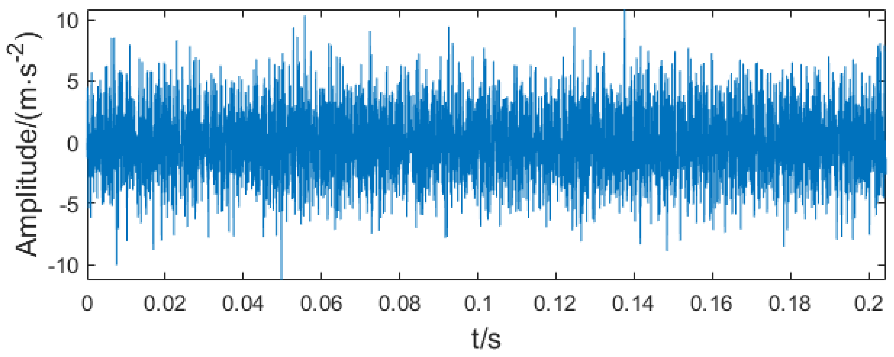
In order to take into account the calculation time and effect, the length of the signal should not be too long or too short. In this paper, 4096 points were selected as the experimental signal, and the sampling frequency was consistent with the parameters used in the laboratory, that is, 25.6 kHz. The time-domain diagram of the experimental signal is shown in Figure 9a, and the envelope diagram is shown in Figure 9b. It can be seen from the time-domain diagram that the original fault impact characteristics cannot be identified under the influence of noise, and the fault information cannot be identified from the time-domain diagram only. From the envelope diagram, only the outer ring fault characteristic frequency of 108 Hz can be observed, while the inner ring fault characteristic frequency and frequency doubling are all covered by noise, which cannot effectively diagnose the fault. Therefore, the experimental signal needs to be processed and then analyzed.
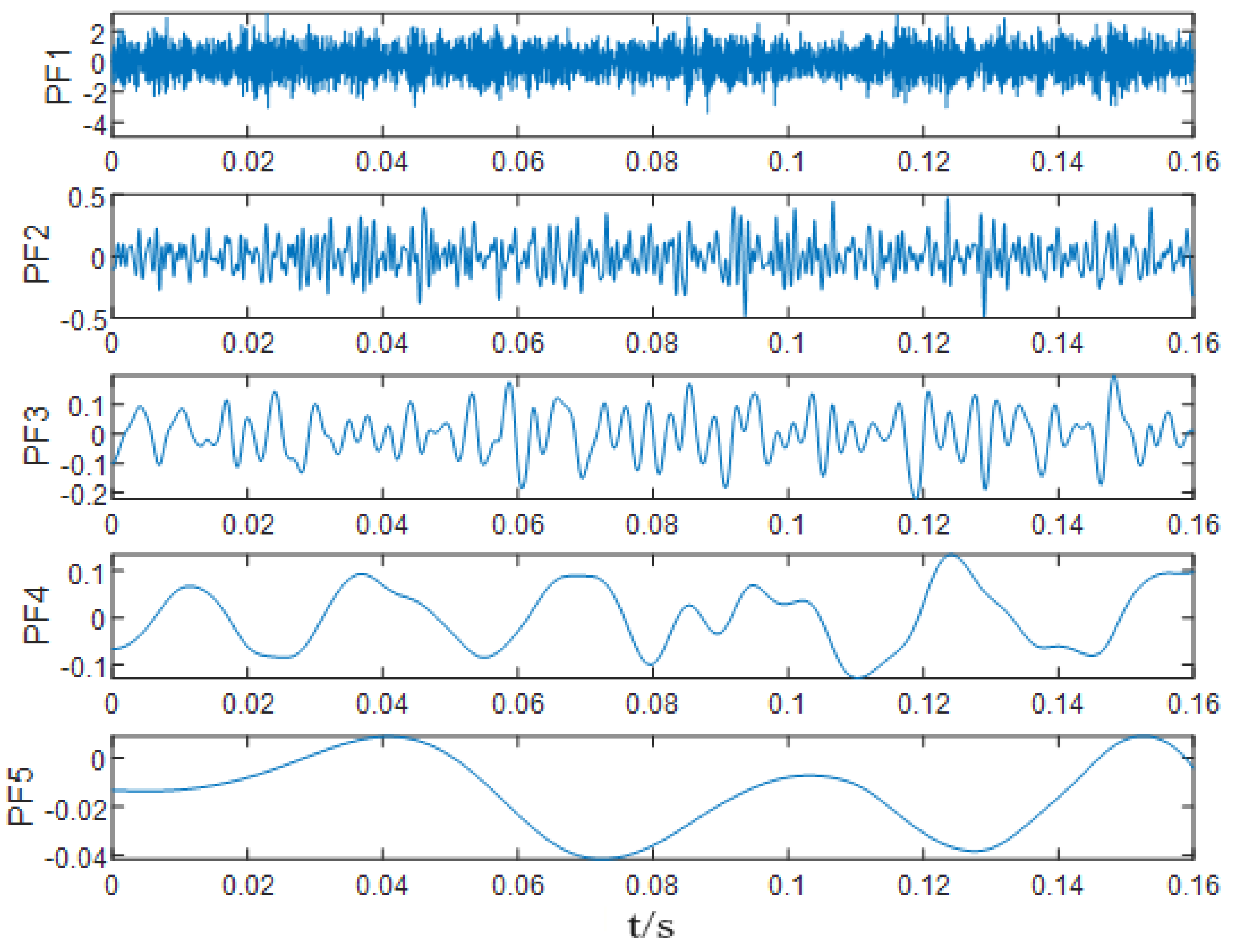
First, the experimental signal is decomposed by RLMD, and several product functions are obtained, as shown in Figure 10. In order to select the components with rich sensitive shock characteristics, the kurtosis value of each component and the correlation coefficient with the original signal are now calculated, as shown in Table 4. It can be seen from the table that the kurtosis values of PF1 and PF2 are large, indicating that they contain more shock characteristics and the correlation coefficient is also high. Therefore, these two components are selected for reconstruction to obtain a reconstructed signal. The time-domain diagram is shown in Figure 11. It can be seen from Figure 11 that the impact components in the signal after component reconstruction are more effectively highlighted compared to Figure 9a, but they are still interfered with by the surrounding noise spectral lines, so the signal needs to be further denoised.
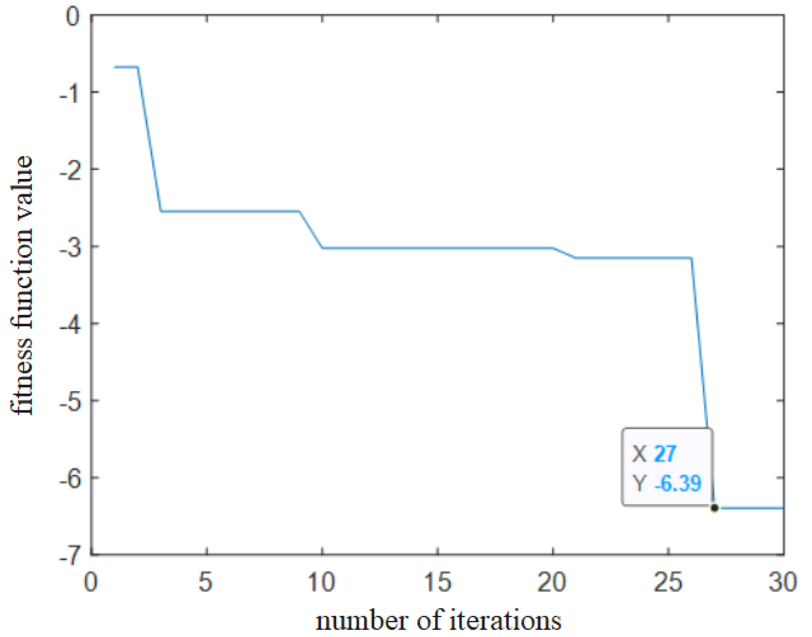
The SSA-CYCBD algorithm is used to denoise and separate the faults of the experimental reconstructed signals. First, the faults of the outer ring are separated. The search range of filter length L is (100, 1000), and the search range of cycle frequency α is (103, 113). As shown in Figure 12, the fitness function -HSI reaches the minimum value when iterating 23 times, and the value is −11.52. At this time, the corresponding parameter [L,α] is (581, 108). The optimal parameters were inputted into the CYCBD algorithm, the simulated signal was deconvolved, and the denoised signal was enveloped. The left side of Figure 13 is the time-domain diagram of the experimental signal after noise reduction, and the right side is the envelope of the experimental signal after noise reduction. From the time-domain diagram, it can be seen that the signal obtained by the reconstructed signal after noise reduction by the SSA-CYCBD algorithm is more obvious than the reconstructed experimental signal. The outer ring fault characteristic frequency of 108 Hz can also be well identified from the envelope diagram, and the double frequency to the ninth frequency of the fault characteristic frequency is also extracted, indicating that the algorithm proposed in this paper can effectively diagnose outer ring failure in compound faults.
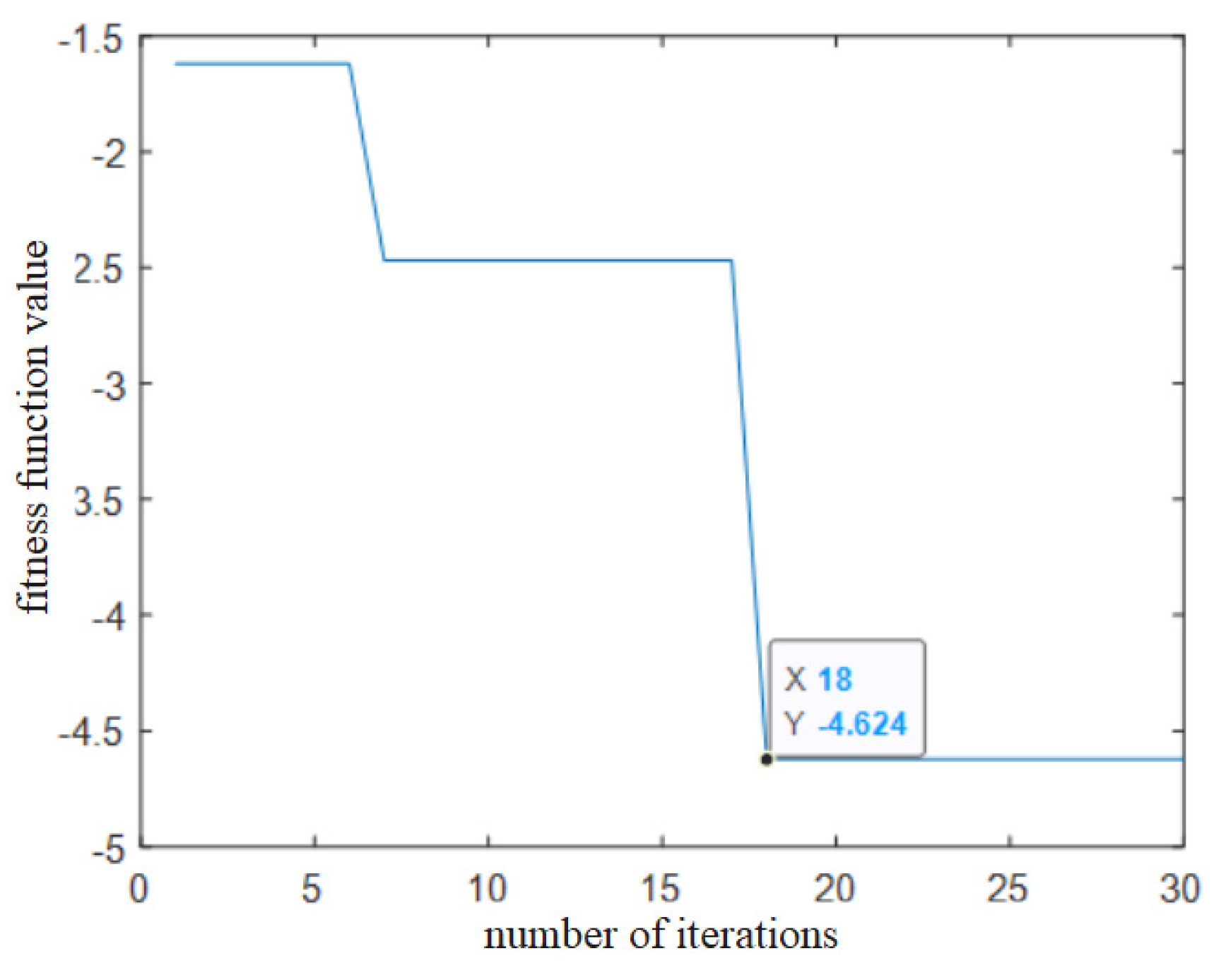
Secondly, the SSA-CYCBD algorithm was used for the RLMD reconstruction experimental signal to separate the inner ring fault. When the search range of the filter length L remains unchanged, the search range of the cycle frequency α becomes (167, 177). The entire diagnosis process is similar to the above-mentioned outer ring fault feature extraction, and will not be described in detail. As shown in Figure 14, the fitness function -HSI reaches the minimum value when iterating 16 times, and the corresponding value was −5.821. At this time, the corresponding parameter [L,α] was (476, 172), and the obtained time-domain diagram and envelope spectrum of the noise reduction signal are shown in Figure 15. The envelope spectrum successfully extracted the fault characteristic frequency of 172 Hz, and the curve from the double frequency to the quadruple frequency of the fault characteristic frequency was prominent; There were obvious peaks, indicating that the algorithm proposed in this paper has the same effect in extracting the inner ring fault in the composite fault experimental signal.

5. Conclusions

This paper proposes a CYCBD algorithm optimization based on RLMD and SSA. RLMD can well separate the signal, extract sensitive components, and complete the primary noise reduction of the signal. CYCBD, which is adaptively optimized by SSA, can enhance the characteristics of different fault types in the composite fault. The simulation signals and laboratory acquisition signals were verified, and good results have been achieved. It is worth noting that the data used in this paper were collected in the laboratory, and the background noise in the actual environment is stronger and more complex, so the model proposed in this paper needs to be optimized and improved to adapt to actual engineering environments. However, in general, this paper still has certain engineering practical value.

Author Contributions

Conceptualization, S.L.; methodology, S.L.; software, S.L.; validation, S.L.; formal analysis, J.M.; investigation, J.M.; resources, J.M.; data curation, J.M.; writing—original draft preparation, S.L.; writing—review and editing, J.M. and S.L.; visualization, J.M.; supervision, J.M.; project administration, J.M.; funding acquisition, J.M. All authors have read and agreed to the published version of the manuscript.

Funding

This research was funded by the National Natural Science Foundation of China under Grant No. 61973041 and the National Key Research and Development Program of China.

Data Availability Statement

The data presented in this study are openly available in the XJTU-SY Bearing dataset at http://biaowang.tech/xjtu-sy-bearing-datasets, accessed on 8 May 2022, reference number [30].

Conflicts of Interest

The authors declare no conflict of interest. The funders had no role in the design of the study; in the collection, analyses, or interpretation of data; in the writing of the manuscript, or in the decision to publish the results.

References

  1. Zhang, K.; Zhou, D.H.; Chai, Y. Review of Composite Fault Diagnosis Technology. Control Theory Appl. 2015, 32, 1143–1157. [Google Scholar]
  2. Zhang, Y.Y.; Jia, Y.X.; Wu, W.Y.; Cheng, Z.H.; Su, X.B.; Lin, A.Q. A diagnosis method for the compound fault of gearboxes based on multi-feature and BP-AdaBoost. Symmetry 2020, 12, 461. [Google Scholar] [CrossRef] [Green Version]
  3. Ma, J.P.; Zhuo, S.; Li, C.W.; Zhan, L.W.; Zhang, G.Z. An enhanced intrinsic time-scale decomposition method based on adaptive lévy noise and its application in bearing fault diagnosis. Symmetry 2021, 13, 617. [Google Scholar] [CrossRef]
  4. Gustantsson, J.G.; Tallian, T. Detection of damage in assembled rolling bearing. Trans. ASLE 1962, 5, 197–209. [Google Scholar] [CrossRef]
  5. Shi, H.T.; Guo, J.; Yuan, Z. Incipient fault detection of rolling element bearings based on deep EMD-PCA algorithm. Shock. Vib. 2020, 2020, 1–17. [Google Scholar] [CrossRef]
  6. Liu, J.; Wang, L.; Tan, H. An extended EEMD method for localized faults detection of a planetary gearbox. J. Test. Eval. 2019, 47, 20180615. [Google Scholar] [CrossRef]
  7. Ma, C.; Wang, S.H.; Xu, X.L. Fault Diagnosis of Acoustic Array Rolling Bearing Based on EEMD. J. Electron. Meas. Instrum. 2017, 31, 1379–1384. [Google Scholar]
  8. Dong, W.; Tsui, K.L.; Yong, Q. Optimization of segmentation fragments in empirical wavelet transform and its applications to extracting industrial bearing fault features. Measurement 2019, 133, 328–340. [Google Scholar]
  9. Liu, C.; Zhang, L.; Niu, J. Intelligent prognostics of machining tools based on adaptive variational mode decomposition and deep learning method with attention mechanism. Neurocomputing 2020, 417, 239–254. [Google Scholar] [CrossRef]
  10. Wang, R.; Xu, L.; Liu, F. Bearing fault diagnosis based on improved VMD and DCNN. J. Vibroengineering 2020, 22, 1055–1068. [Google Scholar] [CrossRef]
  11. Liu, Z.L.; Jin, Y.Q.; Zuo, M.J. Time-frequency representation based on robust local mean decomposition for multicomponent AM-FM signal analysis. Mech. Syst. Signal Process. 2017, 95, 101. [Google Scholar] [CrossRef]
  12. Yan, S.T.; Zhou, Y.G.; Ren, Y.B. Bearing fault diagnosis method based on RLMD and Kmeans++. Mech. Transm. 2021, 45, 163–170. [Google Scholar]
  13. Wiggins, R.A. Minimumentropy deconvolution. Geoexploration 1978, 16, 21–35. [Google Scholar] [CrossRef]
  14. Cheng, Y.; Zhou, N.; Zhang, W. Application of an improved minimum entropy deconvolution method for railway rolling element bearing fault diagnosis. J. Sound Vib. 2018, 425, 53–69. [Google Scholar] [CrossRef]
  15. Chen, J.K.; Chen, X.H. Gear fault diagnosis model combined with MED-LMD-Hypersphere multiclass SVM. In Proceedings of the Prognostics and System Health Management Conference, Chongqing, China, 26–28 October 2018; pp. 1114–1119. [Google Scholar]
  16. Mcdonald, G.L.; Zhao, Q.; Zuo, M.J. Maximum correlated kurtosis deconvolution and application on gear tooth chip fault detection. Mech. Syst. Signal Process. 2012, 33, 237–255. [Google Scholar] [CrossRef]
  17. Li, L.F.; Guo, A.B.; Chen, H.Y. Feature extraction based on EWT with scale space threshold and improved MCKD for fault diagnosis. IEEE Access 2021, 9, 45407–45417. [Google Scholar] [CrossRef]
  18. Ma, T.W.; Zhang, X.F.; Jiang, H. Early fault diagnosis of shaft crack based on double optimization maximum correlated kurtosis deconvolution and variational mode decomposition. IEEE Access 2021, 13, 281–305. [Google Scholar] [CrossRef]
  19. Marco, B.; Jerome, A. Blind deconvolution based on cyclostationarity maximization and its application to fault identification. J. Sound Vib. 2018, 432, 569–601. [Google Scholar]
  20. Rilling, G.; Flandrin, P.; Goncalves, P. On empirical mode decomposition and its algorithms. In Proceedings of the 6th IEEE/EURASIP Workshop on Nonlinear Signal and Image Processing, Grado, Italy, 8–11 June 2003. [Google Scholar]
  21. Shokouhifar, M. Swarm intelligence RFID network planning using multi-antenna readers for asset tracking in hospital environments. Comput. Netw. 2021, 198, 108427. [Google Scholar] [CrossRef]
  22. Shokouhifar, M. FH-ACO: Fuzzy heuristic-based ant colony optimization for joint virtual network function placement and routing. Appl. Soft Comput. 2021, 107, 107401. [Google Scholar] [CrossRef]
  23. Esmaeili, H.; Hakami, V.; Minaei Bidgoli, B. Application-specific clustering in wireless sensor networks using combined fuzzy firefly algorithm and random forest. Expert Syst. Appl. 2022, 210, 118365. [Google Scholar] [CrossRef]
  24. Li, Y.L. Comparative Research on Several New Swarm Intelligence Optimization Algorithms. Comput. Eng. Appl. 2020, 56, 1–12. [Google Scholar]
  25. Zhao, M.; Lin, J.; Miao, Y. Detection and recovery of fault impulses via improved harmonic product spectrum and its application in defect size estimation of train bearings. Measurement 2016, 91, 421–439. [Google Scholar] [CrossRef]
  26. Schroeder, M.R. Period histogram and product spectrum: New methods for fundamental-frequency measurement. Acoust. Soc. Am. 1968, 43, 829–834. [Google Scholar] [CrossRef] [PubMed]
  27. Tang, G.; Wang, X.; He, Y. Diagnosis of compound faults of rolling bearings through adaptive maximum correlated kurtosis deconvolution. J. Mech. Sci. Technol. 2016, 30, 43–54. [Google Scholar] [CrossRef]
  28. Patil, A.P.; Mishra, B.K.; Harsha, S.P. Fault diagnosis of rolling element bearing using autonomous harmonic product spectrum method. Proc. Inst. Mech. Eng. Part K J. Multi-Body Dyn. 2021, 235, 361–411. [Google Scholar] [CrossRef]
  29. Seneff, S. Real-time harmonic pitch detector. IEEE Trans. Acoust. Speech Signal Process. 1976, 26, 358–365. [Google Scholar] [CrossRef] [Green Version]
  30. Wang, B.; Lei, Y.; Li, N. A hybrid prognostics approach for estimating remaining useful life of rolling element bearings. IEEE Trans. Reliab. 2018, 69, 401–412. [Google Scholar] [CrossRef]
  31. Lei, Y.G.; Han, T.Y.; Wang, B. XJTU-SY Rolling Bearing Accelerated Life Test Data Set Interpretation. J. Mech. Eng. 2019, 55, 1–6. [Google Scholar]
  32. Zhou, F.C. Research on Fault Diagnosis Method of Rolling Bearing Based on Cyclostationary Signal Processing; Shanghai Jiaotong University: Shanghai, China, 2006. [Google Scholar]
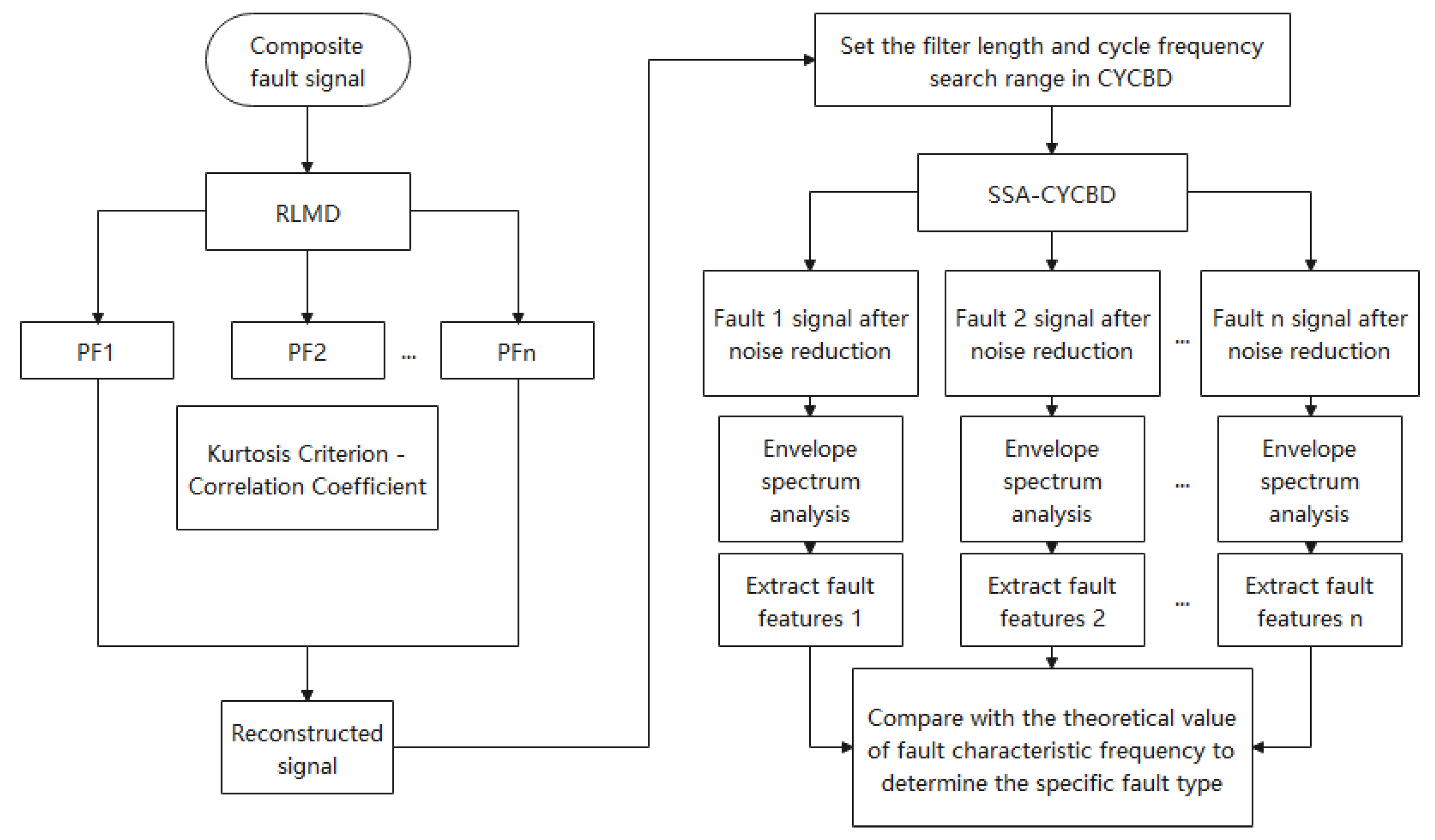
Figure 1. Flow chart of the composite fault diagnosis method combining the RLMD and SSA-CYCBD algorithms.
Processes 10 02208 g001
Figure 2. Simulated composite fault signal time-domain diagram. ((a) The time-domain diagram of inner ring fault signal. (b) The time-domain diagram of outer ring fault signal. (c) The time-domain diagram of noise-added composite fault signal).
Processes 10 02208 g002
Figure 3. The components obtained after the RLMD decomposition of the simulated signal.
Processes 10 02208 g003
Figure 4. Reconstructed signal of the simulated signal.
Processes 10 02208 g004
Figure 5. Fitness function curve of the simulated inner ring signal.
Processes 10 02208 g005
Figure 6. Time-domain and envelope diagrams after SSA-CYCBD enhances the outer ring fault features.
Processes 10 02208 g006
Figure 7. Fitness function curve of the simulated outer ring signal.
Processes 10 02208 g007
Figure 8. Time-domain and envelope maps after SSA-CYCBD-enhancement of inner ring fault features.
Processes 10 02208 g008
Figure 9. Time-domain diagram and envelope diagram of the experimental signal. ((a) Time-domain diagram of experimental signal. (b) Experimental signal envelope).
Processes 10 02208 g009
Figure 10. The components obtained after the RLMD decomposition of the experimental signal.
Processes 10 02208 g010
Figure 11. Time-domain diagram of the reconstructed experimental signal.
Processes 10 02208 g011
Figure 12. Fitness function curve of the outer ring experimental signal.
Processes 10 02208 g012
Figure 13. Time-domain diagram and envelope diagram of the experimental signal after outer ring fault enhancement.
Processes 10 02208 g013
Figure 14. Fitness function curve of the inner ring experimental signal.
Processes 10 02208 g014
Figure 15. Time-domain diagram and envelope diagram of the experimental signal after inner ring fault enhancement.
Processes 10 02208 g015
Table 1. The kurtosis value of each PF component and the correlation coefficient with the original signal.
PFPF1PF2PF3PF4PF5PF6
kurtosis 2.972.872.662.781.931.61
Correlation coefficient0.910.40.160.070.040.04
Table 2. Parameter settings of the SSA.
ParameterValue
group number30
The maximum number of iterations30
number of discoverers10
Be aware of dangerous sparrow numbers5
safety threshold0.8
Table 3. LDK UER204 bearing parameters.
Parameter ValueParameter Value
Inner race diameter29.30 mmBall diameter7.92 mm
Outer race diameter 39.80 mmNumber of balls8
Bearing mean diameter34.55 mmContact angle
Table 4. The kurtosis value from PF1-PF5 component and the correlation coefficient with the original signal.
PFPF1PF2PF3PF4PF5
kurtosis 2.833.342.81.841.93
Correlation coefficient0.980.220.10.080.01
Publisher’s Note: MDPI stays neutral with regard to jurisdictional claims in published maps and institutional affiliations.