Monitoring the Recombinant Adeno-Associated Virus Production using Extended Kalman Filter

Abstract

The recombinant adeno-associated virus (rAAV) is a viral vector technology for gene therapy that is considered the safest and most effective way to repair single-gene abnormalities in non-dividing cells. However, improving the viral titer productivity in rAAV production remains challenging. The first step to this end is to effectively monitor the process state variables (cell density, GLC, GLN, LAC, AMM, and rAAV viral titer) to improve the control performance for an enhanced productivity. However, the current approaches to monitoring are expensive, laborious, and time-consuming. This paper presents an extended Kalman filter (EKF) approach used to monitor the rAAV production using the online viable cell density measurements and estimating the other state variables measured at a low frequency. The proposed EKF uses an unstructured mechanistic kinetic model applicable in the upstream process. Three datasets were used for parameter estimation, calibration, and testing, and the data were collected from the production of rAAV through a triple-plasmid transfection of HEK293SF-3F6 cells. Overall, the proposed approach accurately estimated metabolite concentrations and the rAAV production yield. Therefore, the approach has a high potential to be extended to an online soft sensor and to be classified as a cost-effective and fast approach to the monitoring of rAAV production.

1. Introduction

In general terms, gene therapy is the introduction of a specific cell function through the modification of the cellular genetic material of a patient for the treatment of hereditary or acquired genetic diseases. The effective delivery of genes to the target tissue/cells is carried out using gene delivery vehicles known as vectors, which remains a critical step in gene therapy protocols [1,2]. This area has seen several approved treatments based on viral vectors that vary from vector-based cancer therapies to the treatment of monogenic disorders with life-long benefits [2,3]. The recombinant adeno-associated virus (rAAV) is a versatile viral vector technology for gene therapy applications that may be designed for specific functional interventions. It has proven to be safe and efficient in preclinical and clinical evaluations because of its unique biological and physicochemical features, and rAAV may be employed in a wide range of therapeutic applications in various genetic disorders [1,2,3,4]. Although rAAV is one of the most effective vehicles for directly translating the genomic revolution into medicinal therapies, the manufacturing of rAAV viral vectors remains challenging [5], limiting the generalization of AAV-based treatments.

One of the technological limitations in upstream processing in rAAV manufacturing is the low rAAV yield in large-scale production [5]. Low titers and a high variability in product quality are often the results of an upstream procedure involving an insufficient triple-plasmid transfection of suspension-based cell culture [5]. The situation can be improved by following the Food and Drug Administration’s initiative of process analytical technology (PAT), which requires understanding the process and a timely monitoring of critical process parameters (CPP) that affect critical quality attributes (CQA) [6]. However, current techniques for monitoring the rAAV manufacturing in bioreactors are expensive, laborious, and time-consuming. Sample taking is usually required to measure the CPPs, such as the cell density and metabolites, and the quantification of the CQAs, such as a rAAV genome titer using a quantitative Polymerase Chain Reaction (qPCR)/droplet digital Polymerase Chain Reaction (ddPCR) or a viral capsid titer using an enzyme-linked immunosorbent assay (ELISA), takes one day to complete [7]. Recently, in situ monitoring technologies, such as Raman spectroscopy [8,9] and fluorescence spectroscopy [10,11,12], have been developed to estimate the cell density and metabolites in mammalian cell cultures in real-time, but have not been reported as detecting the rAAV titer. Moreover, the setup of a spectroscopy system is costly in terms of the investment and calibration effort [13]. On the other hand, one solution is to develop fast and cost-effective real-time process monitoring technologies through mathematical models of the production [14,15,16]. Mathematical modeling (MM) is an essential component of process systems engineering (PSE) [17,18,19] and is helpful in monitoring through process state estimation [14,17,20]. Estimation algorithms that rely on the mathematical model can estimate variables that are not directly observable and can predict meaningful process outputs and attributes that are either not measurable online or can only be measured at a low sampling frequency [14,17,19].

The mathematical representations of the rAAV production for state estimation and output prediction can be made with mechanistic kinetic models [21,22,23]. A mechanistic kinetic model can be classified as unstructured and structured [14]. An unstructured model enables the macro-modeling of the functionality of the bioreactor, and it can provide an insight toward the underlying macro-scale phenomena of the upstream process. This kind of model can be used to depict the dynamics of the cell density, viability, nutrient/metabolite concentrations, and product titer [14], which could be determined by online applications (where the data are analyzed in a continuous mode and the sensed variable must be measured more frequently than it can change in the process) and offline applications (where samples are required to be taken and analyzed in the laboratory after proper pre-treatments) [18,24]. Narayanan et al. [21,22] and Fernandes-Platzgummer et al. [23] have used an unstructured model for monoclonal antibody (mAb) production, which is also based on mammalian cell cultures as rAAV production. It is a good starting point for designing a mechanistic model for rAAV production without considering the complexity of the triple-plasmid transfection process. On the other hand, structured mechanistic models are more complex than unstructured ones because they describe details about the intracellular environment of a homogenous cell population [14]. The structured model of rAAV production presented by Nguyen et al. [25] is the first proposed model and is essential for the mechanistic understanding of rAAV production pathways. However, it is not feasible to be extended as an application of soft sensors in bioreactors because it describes the kinetic behavior of transient transfection at the subcellular level. It is most appropriate for cell-line development, where genome-level characteristics of the cells are altered to achieve certain desired process behaviors.

A simple unstructured mechanistic kinetic model (UMKM) has a low prediction ability, and it is not enough to process state estimation because it is improbable that a single set of parameter values enables a kinetic model to satisfactorily for several data sets collected under distinct operating circumstances [26]. Given this, UMKM is commonly implemented with the Kalman filter approach [27] to improve the prediction accuracy and generate predictions in between sampling instances. In various data analysis methods, the Kalman filter and its non-linear extensions, such as the extended Kalman filter, are powerful tools for predicting values of the unobserved states. Although there are several applications of the extended Kalman filter for mAb production [22,28] and other cultivation processes [29,30], its application to the rAAV production process has not been reported.

In this research, an extended Kalman filter (EKF) was proposed to supervise the rAAV production using only online viable cell density (Xv) measurements to estimate the other process state variables, including glucose (GLC) concentration, glutamine (GLN) concentration, lactate (LAC) concentration, ammonium (AMM) concentration, and rAAV viral titers that are measured at a low sampling frequency. The proposed EKF was applied to the cell expansion phase (CEP) and viral vector production phase (VVPP) of the upstream process using a UMKM based on mass balances (only dependent on Xv measurements) as a process model. Three datasets were used in the development of the proposed EKF, and the data were collected from the production of rAAV by a triple-plasmid transfection of HEK293SF-3F6 cells in three different environments: the shake-flasks dataset (offline data), bioreactor 1 dataset (offline data), and bioreactor 2 dataset (online and offline data). The parameters used in the UMKM were estimated with a neural ordinary differential equation and Bayesian inference approaches using the bioreactor 1 dataset. Furthermore, they were also estimated during the execution of EKF using the joint estimation method, and the EKF parameters were obtained from the shake-flasks and bioreactor 1 datasets. Our approach was evaluated with the bioreactor 1 and 2 datasets, and we showed that the proposed approach can only use the online Xv measurements and estimate the GLC, LAC, and rAAV viral titer effectively. The proposed approach is the first EKF approach developed to monitor rAAV production, and it uses only one device as opposed to the current approaches, which require multiple assays/devices. Our results indicate that the proposed EKF has the potential to be generalized and extended to an online soft-sensor, and to be classified as a cost-effective and rapid approach to monitoring rAAV production.

2. Materials and Methods

This section will describe the proposed EKF and the datasets used for calibration and testing.

2.1. Unstructured Mechanistic Kinetic Model Formulation for rAAV Production

The upstream rAAV manufacturing process has four phases: (i) plasmid development, (ii) cell expansion phase, (iii) plasmid transfection, and (iv) viral vector production phase [5]. Our UMKM was designed to apply to the second and fourth phases in a situation that does not have nutrition limitations. The system of ordinary differential equations that compose the proposed unstructured mechanistic model representing the cell culture was established based on mass balances commonly used for monoclonal antibody production [21,22,23]. This strategy was used because both monoclonal antibody production and rAAV production are based on mammalian cell cultures [31,32], and unstructured mechanistic models have been widely employed in monoclonal antibody production using Chinese hamster ovary (CHO) cells to optimize their biomanufacturing [31,33,34].

The system of ordinary differential equations representing the HEK293 cell culture in the cell expansion and viral vector production phases was established based on mass balance Equations (1)–(6) as follows:

$$\begin{array}{cc}\hfill \frac{d{X}_V\left(t\right)}{dt}& ={\mu }_{X_v}{X}_V\left(t\right)\hfill \end{array}$$

(1)

$$\begin{array}{cc}\hfill \frac{dGlc\left(t\right)}{dt}& =-{\mu }_{Glc}{X}_V\left(t\right)\hfill \end{array}$$

(2)

$$\begin{array}{cc}\hfill \frac{dGln\left(t\right)}{dt}& =-{\mu }_{Gln}{X}_V\left(t\right)\hfill \end{array}$$

(3)

$$\begin{array}{cc}\hfill \frac{dLac\left(t\right)}{dt}& ={\mu }_{Lac}{X}_V\left(t\right)\hfill \end{array}$$

(4)

$$\begin{array}{cc}\hfill \frac{dAmm\left(t\right)}{dt}& ={\mu }_{Amm}{X}_V\left(t\right)+k_{deg}Gln\left(t\right)\hfill \end{array}$$

(5)

$$\begin{array}{cc}\hfill \frac{dAAV\left(t\right)}{dt}& ={\mu }_{AAV}{X}_V\left(t\right)\hfill \end{array}$$

(6)

Because the complete metabolic pathway and rAAV production mechanism are unknown, a simplified mass-balance equation system was applied with all variables depending on viable cell (Xv) measurements. This system represents the cell growth, uptake of substrates, metabolism, and production process with six parameters: the specific cell growth rate (${\mu }_{X_v}$), the specific rates of uptake (consumption) of the main nutrients, glucose (${\mu }_{Glc}$) and glutamine (${\mu }_{Gln}$), the specific rates of production of the metabolite waste, lactate (${\mu }_{Lac}$) and ammonium (${\mu }_{Amm}$), and specific rate of production of rAAV (${\mu }_{AAV}$). In the case of ammonium production, the specific rates must consider the spontaneous glutamine degradation in the medium into ammonium [23,35]. This process follows first-order rate kinetics concerning glutamine concentration, $k_{deg}$ being the glutamine degradation constant. Equation (6) enables us to estimate the concentration of viral titer as cell product (quantified as genome copies), where the parameter ${\mu }_{AAV}$ represents the specific rate of rAAV production. The proposed UMKM has two phases. When applied to the cell expansion phase, we considered AAV(t) = 0 and ${\mu }_{AAV}$ = 0, since there is no production of rAAV in this phase. In VVPP, the AAV(t) and ${\mu }_{AAV}$ are different from zero. All parameters used in this work were estimated using EKF and the approaches described in Section 2.3.1 and Section 2.3.2.

2.2. Extended Kalman Filter

The EKF requires a state–space model to perform estimation on the state variables of a process, such as the rAAV production [26,36,37]. A state-space model consists of process and measurement (observation) models [38]. The process model describes the states of the process, including observed and unobserved state variables, and the measurement model describes the relation between the observed variables and the unobserved state variables.

The proposed UMKM (Section 2.1) was used as the process model of EKF, whose purpose is to deal with the non-linear process and measurement models by using linearization based on the first-order Taylor series expansion [26,29]. The EKF can use offline or online measurements of Xv to estimate UMKM state variables value (Xv, GLC, LAC, AMM, and rAAV viral titer) concentrations, as well as UMKM parameters (${\mu }_{X_v},{\mu }_{Glc},{\mu }_{Gln},{\mu }_{Lac},{\mu }_{Amm},k_{deg}$ and ${\mu }_{AAV}$); see Figure 1. The state variables vector to be used by the EKF is composed of the state variables of the UMKM (observed and unobserved) and its parameters. It is called the joint state and parameter estimation method via EKF [28,29,30,37], and the state variables vector is defined as:

$$\mathit{\psi }\left(t\right)={[X_v,GLC,GLN,LAC,AMM,AAV,{\mu }_{X_v},{\mu }_{Glc},{\mu }_{Gln},{\mu }_{Lac},{\mu }_{Amm},k_{deg},{\mu }_{AAV}]}^T.$$

(7)

Subsequently, the process model is represented as

$$\frac{d\mathit{\psi }\left(t\right)}{dt}=\varphi (\mathit{\psi }\left(t\right),t)+\mathit{\omega }\left(t\right),$$

(8)

$$\frac{d}{dt}\left[\begin{array}{c}{X}_V\\ Glc\\ Gln\\ Lac\\ Amm\\ AAV\\ {\mu }_{X_v}\\ {\mu }_{Glc}\\ {\mu }_{Gln}\\ {\mu }_{Lac}\\ {\mu }_{Amm}\\ k_{deg}\\ {\mu }_{AAV}\end{array}\right]=\left[\begin{array}{c}{\mu }_{X_v}{X}_V\\ -{\mu }_{Glc}{X}_V\\ -{\mu }_{Gln}{X}_V\\ {\mu }_{Lac}{X}_V\\ {\mu }_{Amm}{X}_V+k_{deg}Gln\\ {\mu }_{AAV}{X}_V\\ 0\\ 0\\ 0\\ 0\\ 0\\ 0\\ 0\end{array}\right]+\mathit{\omega }\left(t\right)$$

(9)

where $\mathit{\varphi }$ denotes non-linear functions of the state variables in $\mathit{\psi }\left(t\right)$, which corresponds to the proposed UMKM. The UMKM parameters in process model were considered time-dependent and were estimated by adding these parameters as an additional state variable whose differential equation is equal to zero. This procedure that estimates the UMKM parameters was used in [28,29,30]. The process model is formulated in a continuous time t and the white process noise vector is represented by $\mathit{\omega }\sim \mathcal{N}(0,\mathbf{Q})$, with zero mean and error covariance matrix of process model represented by $\mathbf{Q}$.

The measurement model is defined as

$${\mathbf{Z}}_k={\mathbf{H}}_1\mathit{\psi }\left(t_k\right)+\mathit{v},$$

(10)

where the matrix ${\mathbf{H}}_1$ is a linear operator that matches the states variables of $\mathit{\psi }\left(t_k\right)$ to the measured variables ${\mathbf{Z}}_k$ that are obtained at a discrete instance k in a similar way as carried out in [28] and in code available in [29]. In our context, ${\mathbf{H}}_1$ brings only the state variable Xv into the measurement space because only this state variable is measured. The white measurement noise vector is represented by $\mathit{v}\sim \mathcal{N}(0,\mathbf{R})$, with zero mean and measurement noise variance represented by $\mathbf{R}$, since just Xv is measured.

Another important component of EKF process is the state error covariance matrix (P), which contains the error covariance of the predicted state variables values. P can be formulated using linear terms of a Taylor expansion in the continuous-time domain by the following differential equation:

$$\frac{d\mathbf{P}}{dt}=\mathbf{J}\left(t\right)\mathbf{P}\left(t\right)+\mathbf{P}\left(t\right)\mathbf{J}{\left(t\right)}^T+\mathbf{Q}$$

(11)

$$\mathbf{J}\left(t\right)={\left.\frac{\partial \mathit{\varphi }\left(\mathit{\psi }\right(t),t)}{\partial {\mathit{\psi }}_i}\right|}_{\mathit{\psi }=\widehat{\mathit{\psi }}\left(t\right)}$$

(12)

where $\mathbf{J}$ is the Jacobian matrix.

The EKF algorithm was implemented through the prediction step (time update) and correction step (measurement update) [28,29,30,36,37].

Prediction step: Using the initial condition, the predicted state variables vector (${\mathit{\psi }}_{k/k-1}$) and predicted error covariance matrix of state (${\mathbf{P}}_{k|k-1}$) were estimated by solving 9 and 11 from $t_{k-1}$ to $t_k$, where a new measurement is obtained at time k. It is noteworthy that the initial conditions in the prediction step are initial estimation error covariance matrix of state ${\mathbf{P}}_{i,i}(t=0)$, and initial state variables vector $\mathit{\psi }(t=0)$ (composed of state variables and parameters of UMKM).

Correction step: In this step, the estimates of the prediction step (${\mathit{\psi }}_{k/k-1}$ and ${\mathbf{P}}_{k|k-1}$) were combined with the measured value (${\mathbf{Z}}_k$) and Kalman gain (${\mathbf{K}}_k$) to provide corrected state variables vector (${\mathit{\psi }}_{k/k}$) and corrected error covariance matrix of state (${\mathbf{P}}_{k|k}$) using the following equations:

$${\mathbf{K}}_k={\mathbf{P}}_{k|k-1}{\mathbf{H}}_2^T{({\mathbf{H}}_2{\mathbf{P}}_{k|k-1}{\mathbf{H}}_2^T+\mathbf{R})}^{-1}$$

(13)

$${\mathit{\psi }}_{k/k}={\mathit{\psi }}_{k/k-1}+{\mathbf{K}}_k({\mathbf{Z}}_k-{\mathbf{H}}_1{\mathit{\psi }}_{k/k-1})$$

(14)

$${\mathbf{P}}_{k|k}=(\mathbf{I}-{\mathbf{K}}_k{\mathbf{H}}_2){\mathbf{P}}_{k|k-1}$$

(15)

The discrepancy between the true measurements ${\mathbf{Z}}_k$ and the predicted measurement ${\mathbf{H}}_1{\mathit{\psi }}_{k/k-1}$ (that correspond to Xv) was multiplied by the Kalman gain and used to update all predicted state variables in ${\mathit{\psi }}_{k/k-1}$. The matrix ${\mathbf{H}}_2$ is a second linear operator that enables P and K to be updated with information about the UMKM parameters, since we used a simple UMKM, and P and Q with uncorrelated elements. As we wanted to estimate the other state variables and the parameters from the Xv measurements available in discrete time, the ${\mathbf{H}}_2$ used in our case was ${\mathbf{H}}_2$ = diag([1 0 0 0 0 0 1 1 1 1 1 1 0]) in cell expansion phase and ${\mathbf{H}}_2$ = diag([1 0 0 0 0 0 1 1 1 1 1 1 1]) in the viral vector production phase. ${\mathbf{H}}_1$= diag([1 0 0 0 0 0 0 0 0 0 0 0 0]) was used in both phases since we only had Xv measurements.

Using the corrected state variables vector (${\mathit{\psi }}_{k/k}$) and corrected error covariance matrix of state (${\mathbf{P}}_{k|k}$) as initial condition, we could return to the prediction step until the next measurement was obtained and everything repeated again. In addition, the parameters values used in the UMKM and the extended Kalman filter are described in Section 2.5 and in

Table 1. Datasets used in EKF development.

	Shake-Flask Dataset (Runs 1, 2 and 3)	Bioreactor 1 Dataset	Bioreactor 2 Dataset	Bioreactor 2 Dataset
	Offline Measurements	Offline Measurements	Offline Measurements	Online Measurements
	Xv	Xv|GLC|GLN|LAC| AMM|AAV	Xv (CEP) and GLC|LAC|AAV (VVPP)	Xv (CEP and VVPP)
UMKM Parameters Estimation (${\mu }_{X_v}$, ${\mu }_{Glc}$, ${\mu }_{Gln}$, ${\mu }_{Lac}$, ${\mu }_{Amm}$, $k_{deg}$, ${\mu }_{AAV}$)	-	✓	-	-
Initial Estimation Error (IEE) covariance matrix of states (${\mathbf{P}}_{i,i}$)	-	✓	-	-
Error covariance matrix of process model (${\mathbf{Q}}_{i,i}$)	-	✓	-	-
Measurement noise variance R	✓	-	-	-
EKF Calibration	-	✓	-	-
EKF Test	-	-	✓	✓

.

2.3. ODE Parameter Estimation Approaches

The parameter estimation of a system of ODEs is a problem that necessitates finding the solution to a dynamic optimization problem, which is a non-convex problem that generally demands global optimization methods [39]. In this work, we used neural ordinary differential equation (NODE) and Bayesian inference approaches to estimate the parameters of the proposed UMKM. The main reason is to increase the robustness of results because findings can be strengthened when different methods generate results that converge and are found to be congruent. Consequently, this can increase confidence regarding the findings. NODE is a method used for learning time-continuous dynamics from data in the form of a system of ordinary differential equations. It is a particularly promising approach for learning latent dynamics of dynamical systems. NODE naturally fits well as a latent dynamics model in reduced-order modeling of physical processes because it learns the latent dynamics in the form of ODEs [40]. Furthermore, NODE is flexible in learning from irregularly sampled time-series data [40,41,42,43]. Including ODE in NODE enables optimizing and obtaining the point estimates for the best parameters of ODE. However, data have noise, and we need to generate a fit with some uncertainty, which is necessary for uncertainty quantification [44,45]. This can be carried out with Bayesian inference because it enables parameter estimation with quantified uncertainty, which can be represented by mean ± Standard Deviation (StD). It is noteworthy that the UMKM parameters estimated by Bayesian inference are used as initial UMKM parameters in the state variables vector of EKF to be updated during the process using the joint state and parameter estimation method described in Section 2.2.

2.3.1. Neural Ordinary Differential Equation

NODE is a family of neural network models in which one or some hidden layers are implemented with an ordinary differential equation solver. In NODEs, the forward and backward propagation rely on solving an ODE and its adjoint equation [41,42,43]. Therefore, a neural network able to approximate the ordinary differential equation of the dynamical system is called a NODE [46]. It models the dynamics of the hidden feature state $\mathbf{h}\left(t\right)\in {\mathbb{R}}^N$ using an ODE that is parametrized by a derivative model (neural network) $f(\mathbf{h}\left(t\right),t,\theta )\in {\mathbb{R}}^N$ with learnable parameters $\theta =[{\mu }_{X_v},{\mu }_{Glc},{\mu }_{Gln},{\mu }_{Lac},{\mu }_{Amm},k_{deg},{\mu }_{AAV}]$ as follows:

$$\begin{array}{c}\hfill \frac{d\mathbf{h}\left(t\right)}{dt}=f(\mathbf{h}\left(t\right),t,\theta ).\end{array}$$

(16)

Therefore, NODEs are composed of a derivative model $f\left(\mathbf{h}\right(t),t,\theta )$ used to compute the dynamics of hidden layer at a given time $t\in [t_0,t_n]$, a set of parameter $\theta$, and a time interval, $[t_0,t_n]$, in order to evaluate them. NODEs obtain the solution of ODE,

$$\begin{array}{c}\hfill \mathbf{h}\left(t_n\right)={[X_V\left(t_n\right),Glc\left(t_n\right),Gln\left(t_n\right),Lac\left(t_n\right),Amm\left(t_n\right),AAV\left(t_n\right)]}^T,\end{array}$$

(17)

by integrating the derivative model over the time span as follows:

$$\begin{array}{c}\hfill \mathbf{h}\left(t_n\right)=\mathbf{h}\left(t_0\right)+{\int }_{t_0}^{t_n}f(\mathbf{h}\left(t\right),t,\theta )dt,\end{array}$$

(18)

Then, using a black-box numerical ODE solver, we obtained

$$\begin{array}{c}\hfill \mathbf{h}\left(t_n\right)=ODESolve(\mathbf{h}\left(t_0\right),f,\theta \left(t\right),t_0,t_n)\end{array}$$

(19)

where $\mathbf{h}\left(t_0\right)$ represents the initial condition of system of ODE. The ultimate objective is for $\mathbf{h}\left(t\right)$ to get as close to the desired observed data ${\mathbf{y}}_{obs}\left(t\right)$ (discrete measurements) as possible:

$$\begin{array}{c}\hfill {\mathbf{y}}_{obs}\left(t\right)={[X_{Vobs}\left(t\right),Gl{c}_{obs}\left(t\right),Gl{n}_{obs}\left(t\right),La{c}_{obs}\left(t\right),Am{m}_{obs}\left(t\right),AA{V}_{obs}\left(t\right)]}^T.\end{array}$$

(20)

Thus, a loss function is needed to assess the performance of NODEs at each iteration. In this work, we included the system of ODE in a single-layer neural network that takes the parameters $\theta$ and returns the solution of the state variables $X_V\left(t\right),Glc\left(t\right),Gln\left(t\right),Lac\left(t\right),Amm\left(t\right)$ and $AAV\left(t\right)$. Then, using the mean square error loss function defined as

$$\begin{array}{c}\\ L({\mu }_{X_v},{\mu }_{Glc},{\mu }_{Gln},{\mu }_{Lac},{\mu }_{Amm},k_{deg},{\mu }_{AAV})=\\ \Vert log\left(\mathbf{h}\left(t\right)\right)-log\left({\mathbf{y}}_{obs}\left(t\right)\right){\Vert }^2=\\ \Vert log\left(X_{V_h}\left(t\right)\right)-log\left(X_{V_{obs}}\left(t\right)\right){\Vert }^2\\ +\Vert log\left(Gl{c}_h\left(t\right)\right)-log\left(Gl{c}_{obs}\left(t\right)\right){\Vert }^2\\ +\Vert log\left(Gl{n}_h\left(t\right)\right)-log\left(Gl{n}_{obs}\left(t\right)\right){\Vert }^2\\ +\Vert log\left(La{c}_h\left(t\right)\right)-log\left(La{c}_{obs}\left(t\right)\right){\Vert }^2\\ +\Vert log\left(Am{m}_h\left(t\right)\right)-log\left(Am{m}_{obs}\left(t\right)\right){\Vert }^2\\ +\Vert log\left(AA{V}_h\left(t\right)\right)-log\left(AA{V}_{obs}\left(t\right)\right){\Vert }^2,\end{array}$$

(21)

We trained the NODE to arrive at optimal parameters that make the solution of ODE system near to observed values of the train set (bioreactor 1 dataset). Minimization was carried out through local adjoint sensitivity analysis following a similar procedure outlined in [41] and implemented using the adaptive differential evolution optimizer with 2500 iterations and with the strategy rand/1/bin with radius limited sampling (the word “rand” indicates that the individuals selected to compute the mutation values are chosen at random, “1” is the number of pairs of individuals chosen, and, finally, “bin” means that a binomial crossover is used) [47,48].

2.3.2. Bayesian Inference Parameters Estimation

Bayesian inference provides a robust approach toward parameter estimation with quantified uncertainty using a posterior distribution. In the Bayesian framework, beliefs about a parameter are described by a posterior distribution:

$$p\left(\theta \right|{\mathbf{y}}_{obs})\propto p\left({\mathbf{y}}_{obs}\right|\theta )p\left(\theta \right).$$

(22)

The posterior distribution, Equation (22), is a probability distribution for model parameter values, $\theta =[{\mu }_{X_v},{\mu }_{Glc},{\mu }_{Gln},{\mu }_{Lac},{\mu }_{Amm},k_{deg},{\mu }_{AAV}]$ (unknown parameters), conditioned on observational data ${\mathbf{y}}_{obs}$. It is proportional to the likelihood, $p\left({\mathbf{y}}_{obs}\right|\theta )$, times the prior, $p\left(\theta \right)$ [44,45]. Equation (22) allows us to learn model parameters from data by incorporating prior knowledge with likelihood and sampling model parameters from the corresponding posterior distribution. Markov chain Monte Carlo (MCMC) methods were used to generate a sufficient quantity of samples from the posterior distribution, such that the properties of the posterior distribution can be estimated through the generated samples. In our case, the observed data used to estimated the parameters came from bioreactor 1 dataset, (${\mathbf{y}}_{obs}=Datase{t}_{Bioreactor1}$), and the likelihood is the ODE solver with probabilistic parameters $\theta$, defined as

$$p\left({\mathbf{y}}_{obs}\right|\theta )=ODESolve(\mathbf{h}\left(t_0\right),f,\theta \left(t\right),t_0,t_n).$$

(23)

Aiming to find the distributions of the parameters $p\left(\theta \right|{\mathbf{y}}_{obs})$ to obtain their mean and StD, the No-U-Turn-Sampler (NUTS) was used [44,45]. It is an extension of the Hamiltonian Monte Carlo (HMC) algorithm, which is MCMC method. In the NUTS algorithm, we used 2000 iterations to run it and a target acceptance rate of 0.65. In this work, we used Turing, Distributions, and DifferentialEquations.jl Julia packages to solve and estimate the parameters of the metabolic equations [45].

2.4. Datasets

2.4.1. Data Description

The data were collected from the production of rAAV through triple-plasmid transfection of HEK293SF-3F6 cells (National Research Council Canada, Montreal, QC, Canada) in three shake-flasks and two bioreactors. In the shake-flasks experiments, rAAV6 vectors were produced, whereas, in the first bioreactor, rAAV9 vectors were produced, and in the second bioreactor, rAAV6 vectors were produced. The triple-plasmid transfections were completed following the methods previously described in the literature [49].

2.4.2. Shake-Flasks Dataset

Three 250 mL samples of cells culture with starting viable cell density between 0.58–0.73 ×${10}^6$ cells/mL in HycellTM TransFxTM medium added with 6 mM of L-glutamine (Cytiva Life Sciences, Chicago, IL, USA) were cultured in shake-flasks. The cells were incubated at 37 °C, 5% CO₂ in a shaker incubator (Infors, Basel, Switzerland) at 120 rpm agitation rate and transfected at 36 h post inoculation (hpi) with the viable cell density at around $1\times {10}^6$ cells/mL for all runs. The shake-flasks were harvested at 84 hpi (48 h post transfection). Samples were taken every 12 h until harvest.

2.4.3. Bioreactor 1 Dataset

The bioreactor production was carried out in a 3 L bioreactor with a 2.7 L working volume controlled by a my-Control controller (Applikon Biotechnology, Delft, the Netherlands). The dissolved oxygen was maintained above 40% by the oxygen supply PID control loop at a stirring rate of 90 RPM. The pH was maintained at 7.2 by CO₂ overlay and sodium bicarbonate addition PID control loop. The temperature was maintained at 37 °C using a heating jacket. Cells were inoculated into a bioreactor with an initial viable cell density of $0.36\times {10}^6$ cells/mL in the same medium as the shake-flasks experiment. The cells were transfected at 57 hpi with viable cell density at $1.27\times {10}^6$ cells/mL. The bioreactor was harvested at 114 hpi (61 hpt). Samples were taken approximately every 24 h before transfection and approximately 12 h after transfection until harvest.

2.4.4. Bioreactor 2 Dataset

Bioreactor 2 was cultivated under same setup as bioreactor 1. Cells were inoculated with initial viable cell density of 0.27 ×${10}^6$ cells/mL in the same medium. The cells were transfected at 53 hpi with viable cell density at 1.03 ×${10}^6$ cells/mL. The bioreactor was harvested at 102 hpi (49 hpt). Samples were taken approximately every 24 h.

2.4.5. Current Approach: Quantitative Analysis

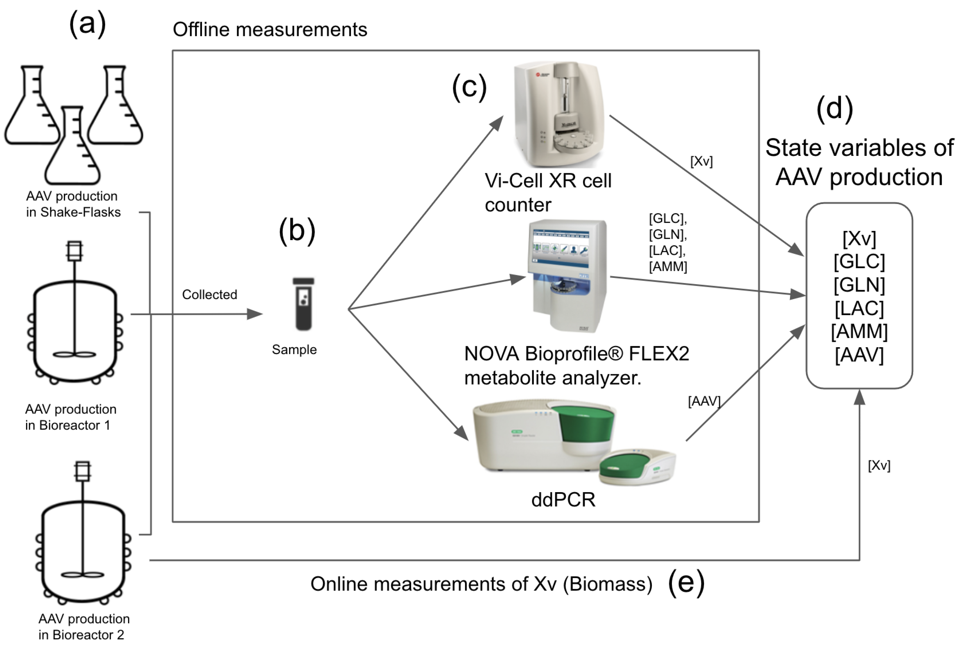
Figure 2 shows the quantitative analysis performed using current approaches that allow for the rAAV production monitoring. The online viable cell density of bioreactor 2 was monitored by a capacitance probe (FUTURA ABER, Aberystwyth, UK) at a recording interval of 1 min. The probe reading was zeroed in pure medium and calibrated at a cell density of 1 ×${10}^6$ cells/mL. Offline viable cell density and metabolites were measured with Vi-Cell XR cell counter (Beckman Coulter, Brea, CA, USA) and Bioprofile® FLEX2 metabolite analyzer (NOVA Biomedical, Waltham, MA, USA), respectively, right after the sample was taken. Offline samples for vector genome (vg) copies quantification by ddPCR were frozen at -80 degrees after being taken. On the day of quantification, the sample was thawed and harvested before viral DNA extraction with a High Pure Viral DNA Extraction kit (Roche Diagnostics, Risch-Rotkreuz, Switzerland). The harvest and ddPCR were carried out following the methods in the literature [49].

It is noteworthy that the offline quantification of Xv, GLC, GLN, LAC, and AMM takes around 30 min to obtain one set of data point at specific time t. However, the quantification of viral titer in rAAV production was carried out only at the end of production. After the production was completed, the samples collected were used to quantify the viral titer and the ddPCR, which took 1 day to complete the process.

2.5. Parameters of the UMKM and the Extended Kalman Filter

The datasets used to obtain the UMKM parameters (${\mu }_{X_v}$, ${\mu }_{Glc}$, ${\mu }_{Gln}$, ${\mu }_{Lac}$, ${\mu }_{Amm}$, $k_{deg}$, ${\mu }_{AAV}$) and the EKF parameters (R, P, and Q) are presented in Table 1. We estimated the parameters of the UMKM for the cell expansion and viral vector production phases with two different approaches, NODE and Bayesian inference, using the bioreactor 1 dataset, and the results of these approaches are discussed in Section 3.1.

The UMKM parameters were also estimated by the EKF during its execution (using the joint estimation method). This is important because this can enable the EKF to better estimate the state variables in different datasets. However, to this end, the EKF parameters should be well defined. The initial estimation error (IEE) covariance matrix of states (${\mathbf{P}}_{i,i}$) and error covariance matrix of process model (${\mathbf{Q}}_{i,i}$) (parameters of EKF) were assumed constant and uncorrelated. This means that these covariance matrices are constant and diagonal, and the diagonal elements are noise variances. These simplification assumptions are common due to the limited data [28,29,30]. The IEE covariance matrix (${\mathbf{P}}_{i,i}$) was assumed diagonal with zero variances for all UMKM metabolic states variables (Xv, GLC, LAC, AMM, and rAAV viral titer), since actual data were used for the initial point. However, the ${\mathbf{P}}_{i,i}$ values regarding the UMKM parameters (${\mu }_{X_v}$,${\mu }_{Glc}$,${\mu }_{Gln}$,${\mu }_{Lac}$,${\mu }_{Amm}$,$k_{deg}$,${\mu }_{AAV}$) were obtained in the calibration of EKF (Section 2.6.1 and Section 3.2). The diagonal values of the ${\mathbf{Q}}_{i,i}$ regarding the UMKM parameters were obtained similarly (Section 2.6.1 and Section 3.2); however, the values regarding all metabolic states were considered different from zero but lower than the measurement noise variance ($\mathbf{R}$) that was obtained from the variance of Xv measurements in the shake-flask dataset regards three runs, see Table 1. Please note that R represents only the variance of Xv, since only Xv is measured, and is therefore one-dimensional.

2.6. Evaluation

The evaluation aims to check the potential of the proposed EKF to estimate the state variables of rAAV production using only the Xv measurements. Therefore, the main result of the evaluation comes from the EKF test using a realistic scenario where online measurement of Xv must be used to estimate the other state variables of rAAV manufacturing in CEP and VVPP. It is essential to point out that the EKF test depends on the UMKM parameters estimated by the Bayesian inference to be used as the initial condition in the state variables vector $\mathit{\psi }(t=0)$, and on the calibration of EKF to obtain ${\mathbf{P}}_{i,i}(t=0)$ and ${\mathbf{Q}}_{i,i}$.

2.6.1. Calibration Using Offline Values

Model calibration is the process of identifying a set of optimal model parameters that accurately describe the behavior of a system. It is accomplished by comparing model predictions to reference data taken on the system [50]. It can be carried out manually using parameter adjustments when we have a start point near the optimal model parameters [51]. In this work, the EKF calibration aimed to identify the final values for the parameters ${\mathbf{P}}_{i,i}(t=0)$ and ${\mathbf{Q}}_{i,i}$ regarding the (${\mu }_{X_v}$, ${\mu }_{Glc}$, ${\mu }_{Gln}$, ${\mu }_{Lac}$, ${\mu }_{Amm}$, $k_{deg}$, ${\mu }_{AAV}$) that enables EKF to use the measurement of Xv and estimate the other state variables. The reference data used in the calibration were the observed data from the bioreactor 1 dataset. Furthermore, the initial observed data from the bioreactor 1 dataset were used as the initial conditions of the state variable vector, see

Table 2. Initial conditions of state variables in CEP and VVPP for the EKF calibration using bioreactor 1 dataset.

State Variables	Name	Value in CEP	Value in VVPP 1
Xv	Viable cells	0.36 × ${10}^6$ c/mL	1.27 × ${10}^6$ c/mL
GLC	Glucose	32.19 mM	24.1 mM
GLN	Glutamine	5.03 mM	3.54 mM
LAC	Lactate	0.111 mM	7.88 mM
AMM	Ammonium	0.33 mM	1.46 mM
AAV	AAV viral titer	0 VG/mL	0 VG/mL

¹ The VVPP values are different from CEP values because they are different phases of upstream process.

. This dataset has only offline measurements of all-state variables; see Table 1. The calibration was performed manually, considering the variance computed from the standard deviation (StD) obtained by Bayesian inference to estimate UMKM parameters (Section 3.1) as the start point near the optimal EKF parameters (${\mathbf{P}}_{i,i}(t=0)$ and ${\mathbf{Q}}_{i,i}$). It is a challenging task to properly estimate ${\mathbf{P}}_{i,i}(t=0)$ and ${\mathbf{Q}}_{i,i}$ due to the limited amount of data. Therefore, these manual calibration and simplification assumptions were made to estimate these errors. Furthermore, we evaluated the calibration obtained by comparing the prediction of UMKM (with estimated parameters by Bayesian inference) and EKF. The root means square error (RMSE) was used as a metric to assess the similarity between their predictions and the observed values of offline measurements of the bioreactor 1 dataset.

2.6.2. EKF Test

The goal of the EKF test is to assess the performance of the proposed EKF in estimating the rAAV production states from online measurements of Xv in VVPP. Estimates close to the reference data (observed data) represent a good performance of the EKF and indicate that the proposed EKF can reduce the demand for the offline analysis required by the current approaches for monitoring rAAV production. The EKF test uses the final set of parameters ${\mathbf{P}}_{i,i}(t=0)$ and ${\mathbf{Q}}_{i,i}$ obtained in the calibration (as well as the $\mathbf{R}$), and an initial state variables vector $\mathit{\psi }(t=0)$ composed of UMKM parameters estimated by Bayesian inference. The EKF test was performed with the bioreactor 2 dataset with four key process parameters: online measurements of Xv and offline measurements of GLC, LAC, and rAAV (where the sampling frequency is approximately every 24 h); see Table 1. The online measurements were input into the proposed EKF to estimate the state variables, and the offline measurements were used as reference data to assess the EKF estimation. It is important to point out that the initial condition of UMKM state variables in CEP that compose the initial state variables vector $\mathit{\psi }(t=0)$ came from the bioreactor 2 dataset, but the final concentration of state variables estimated by EKF in CEP was considered as the initial concentration of UMKM state variables in VVPP that compose the initial state variables vector $\mathit{\psi }(t=0)$ in that phase. Furthermore, the EKF was applied in a different dataset that was used to estimate UMKM parameters (bioreactor 1 dataset). Here, different from the calibration, it was not expected that UMKM could predict the bioreactor 2 dataset well with the parameters estimated from the bioreactor 1 dataset during the entire process. On the other hand, the EKF was expected to outperform the UMKM when estimating the state variables related to the bioreactor 2 dataset because it can update the UMKM parameters during the execution. The RMSE was also used as a metric to evaluate the similarity of EKF estimation and the offline measurements of the bioreactor 2 dataset.

3. Results

The results of this work are presented in the following sequence: parameter estimation, calibration, and the testing of EKF. This sequence was chosen because, in order to perform the EKF test, it is necessary to use the results of the Bayesian parameter estimation for UMKM and the calibration of EKF.

3.1. UMKM Parameter Estimation with NODE and Bayesian Inference

The loss functions in the training processes of NODE with regard to UMKM converged to a minimum before 2000 iterations in CEP, and 1500 iterations in VVPP; see Figure S1. The chains obtained with the NUTS sampler in Bayesian inference were sufficiently converged. This was verified with the auto-correlation function (ACF) plot. It is a valuable diagnostic for assessing the chain mixing rate. Figures S2 and S3 show the marginal posterior distributions for the parameters of UMKM in CEP and VVPP and the respective ACF plots. The ACF values quickly dropped to zero, indicating the good quality of the mixing obtained with the NUT sampler. Furthermore, the parameters estimated with the NODE and Bayesian approaches showed a high similarity with the parameter values estimated by the NODE approach within the range of the variation (mean ± StD) estimated by the Bayesian approach; see

Table 3. Estimated parameters for the UMKM in cell expansion phase (CEP) and viral vector production phase (VVPP) by NODE and Bayesian inference.

	NODE		Bayesian Inference
Parameter	CEP	VVPP	CEP (Mean)	CEP (StD)	VVPP (Mean)	VVPP (StD)
${\mu }_{Xv}$ (h${}^{-1}$)	0.0295	0.0068	0.0299	0.0004	0.0065	0.0003
${\mu }_{GLC}$ $\left(\mathrm{mmol}{10}^{-6}\mathrm{c}{\mathrm{h}}^{-1}\right)$	0.1850	0.0955	0.1895	0.0028	0.0973	0.0050
${\mu }_{GLN}$ $\left(\mathrm{mmol}{10}^{-6}\mathrm{c}{\mathrm{h}}^{-1}\right)$	0.0329	0.0172	0.0350	0.0030	0.0213	0.0031
${\mu }_{LAC}$ $\left(\mathrm{mmol}{10}^{-6}\mathrm{c}{\mathrm{h}}^{-1}\right)$	0.2500	0.0243	0.2544	0.0045	0.0214	0.0031
${\mu }_{AMM}$ $\left(\mathrm{mmol}{10}^{-6}\mathrm{c}{\mathrm{h}}^{-1}\right)$	${10}^{-5}$	0.0001	0.0001	0.0001	0.0001	2.9 × ${10}^{-5}$
$k_{deg}$ (h${}^{-1}$)	0.0050	0.0022	0.0049	0.0001	0.0020	0.0003
${\mu }_{AAV}$ $({10}^9\mathrm{vg}/\mathrm{mL}\mathrm{h}{10}^6\mathrm{c})$	0	0.0622	0	0	0.0644	0.0027

. It is noteworthy that Bayesian inference results were used as an initial condition in the state variables vector $\mathit{\psi }(t=0)$ (columns 4 and 6 of Table 3), and in the calibration of EKF, to obtain ${\mathbf{P}}_{i,i}(t=0)$ and ${\mathbf{Q}}_{i,i}$ (columns 5 and 7 of Table 3).

3.2. EKF Calibration

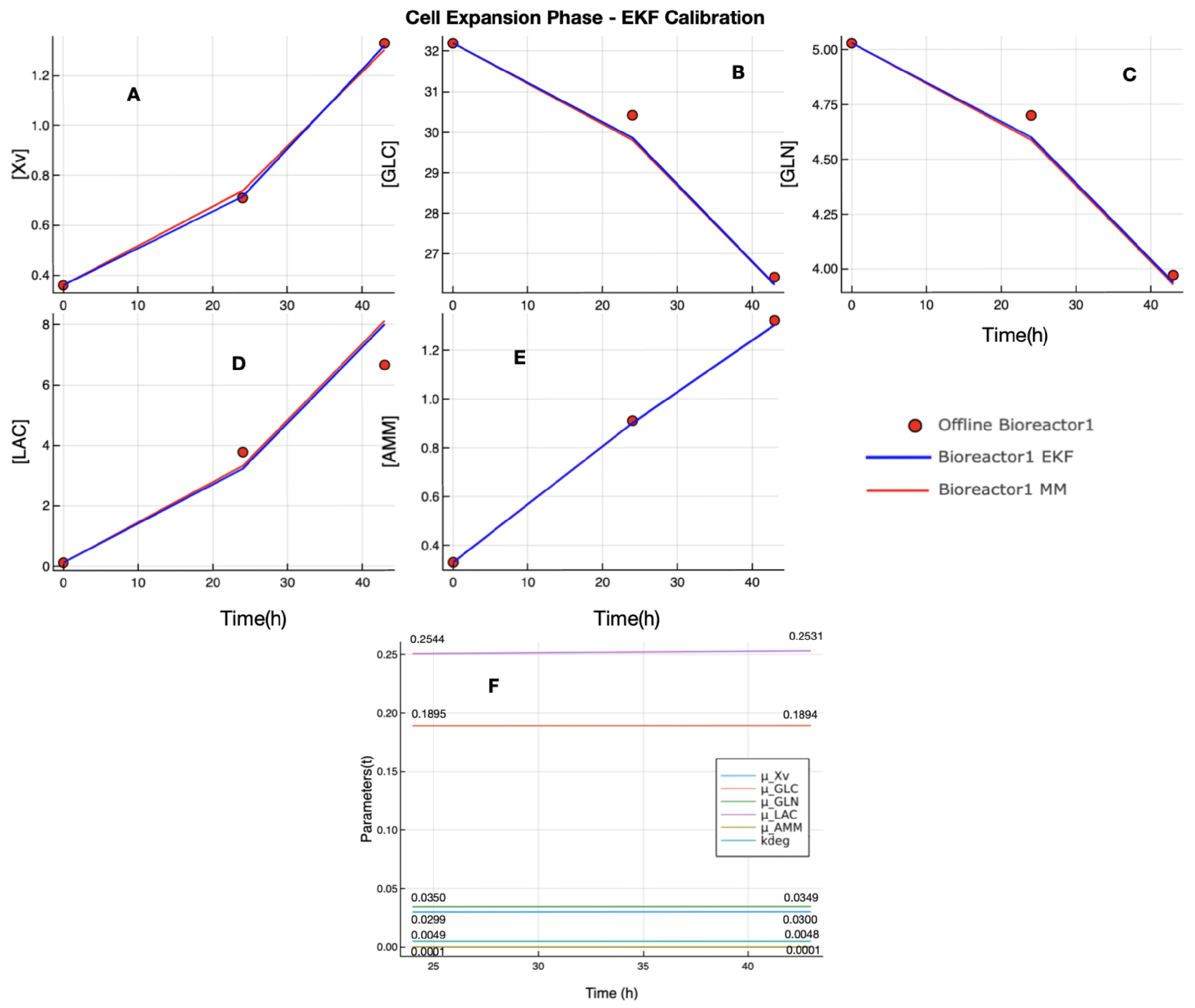
Figure 3 presents the results of the calibration of EKF regarding the cell expansion phase. In this case, the offline measurements of Xv (plot A) from the bioreactor 1 dataset do not have measurements that can be considered as outliers, and the EKF estimation followed the offline observed data and estimation of UMKM. The offline measurements of the other state variables have a small amount of noise, but they are not considered outliers; see the red points in Figure 3, plots B, C, D, and E. The plots show that the proposed EKF performs similarly to UMKM in estimating the state variables in CEP, which is confirmed by the similar RMSE values of the proposed EKF and UMKM estimations regarding the offline measurements of the bioreactor 1 dataset; see

Table 4. RMSE values of the EKF and UMKM estimations regards bioreactor 1 dataset in the calibration.

		EKF	EKF	UMKM	UMKM
State Variables	Name	RMSE Value in CEP	RMSE Value in VVPP	RMSE Value in CEP	RMSE Value in VVPP
Xv	Viable cells	0.009	0.235	0.027	0.258
GLC	Glucose	0.425	1.529	0.456	1.47
GLN	Glutamine	0.076	0.367	0.085	0.363
LAC	Lactate	1.021	0.655	1.082	0.635
AMM	Ammonium	0.014	0.123	0.015	0.12
AAV	AAV viral titer	-	0.722	-	0.819

. In addition, the UMKM parameters (${\mu }_{X_v},{\mu }_{Glc},{\mu }_{Gln},{\mu }_{Lac},{\mu }_{Amm},k_{deg},{\mu }_{AAV}$) estimated by EKF during the process do not present a significant discrepancy from the parameters estimated by Bayesian inference using the bioreactor 1 dataset. This result was expected, since the parameters estimated by Bayesian inference were used as initial UMKM parameters by EKF, and these parameters enabled the process model of EKF (UMKM) to perform estimation near the observed data of the bioreactor 1 dataset. In plot F, Figure 3, we can see that the parameters do not change significantly during the EKF process. The final values of ${\mathbf{P}}_{i,i}(t=0)$ and ${\mathbf{Q}}_{i,i}$ (as well as $\mathbf{R}$) used in the calibration of EKF in CEP are presented in the

Table 5. Initial estimation error (IEE) covariance matrix ${\mathbf{P}}_{i,i}$ for EKF.

Parameter	Name	Value in CEP	Value in VVPP
${\mathrm{P}}_{1,1}({\mathrm{c}}^2/{\mathrm{mL}}^2)$	Viable cells IEE	0.00	0.00
${\mathrm{P}}_{2,2}\left({\mathrm{mM}}^2\right)$	Glucose IEE	0.00	0.00
${\mathrm{P}}_{3,3}\left({\mathrm{mM}}^2\right)$	Glutamine IEE	0.00	0.00
${\mathrm{P}}_{4,4}\left({\mathrm{mM}}^2\right)$	Lactate IEE	0.00	0.00
${\mathrm{P}}_{5,5}\left({\mathrm{mM}}^2\right)$	Ammonium IEE	0.00	0.00
${\mathrm{P}}_{6,6}({\mathrm{VG}}^2/{\mathrm{mL}}^2)$	AAV viral titer IEE	0.00	0.00
${\mathrm{P}}_{7,7}\left({\mathrm{h}}^{-2}\right)$	${\mu }_{Xv}$ IEE	1.71 × ${10}^{-6}$	7.92 × ${10}^{-7}$
${\mathrm{P}}_{8,8}\left(\mathrm{mmol}{10}^{-12}\mathrm{c}{\mathrm{h}}^{-2}\right)$	${\mu }_{GLC}$  IEE	1.53 × ${10}^{-6}$	2.56 × ${10}^{-5}$
${\mathrm{P}}_{9,9}\left(\mathrm{mmol}{10}^{-12}\mathrm{c}{\mathrm{h}}^{-2}\right)$	${\mu }_{GLN}$  IEE	1.81 × ${10}^{-6}$	1.05 × ${10}^{-5}$
${\mathrm{P}}_{10,10}\left(\mathrm{mmol}{10}^{-12}\mathrm{c}{\mathrm{h}}^{-2}\right)$	${\mu }_{LAC}$  IEE	2.55 × ${10}^{-5}$	9.59 × ${10}^{-6}$
${\mathrm{P}}_{11,11}\left(\mathrm{mmol}{10}^{-12}\mathrm{c}{\mathrm{h}}^{-2}\right)$	${\mu }_{AMM}$  IEE	2.97 × ${10}^{-9}$	6.71 × ${10}^{-10}$
${\mathrm{P}}_{12,12}\left({\mathrm{h}}^{-2}\right)$	$k_{deg}$  IEE	3.37 × ${10}^{-9}$	8.71 × ${10}^{-8}$
${\mathrm{P}}_{13,13}({\mathrm{vg}}^2/{\mathrm{mL}}^2{\mathrm{h}}^2{10}^{12}\mathrm{c})$	${\mu }_{AAV}$ IEE	0	4.30 × ${10}^{-6}$

and

Table 6. Measurement noise variance R and error covariance matrix of process model ${\mathbf{Q}}_{i,i}$ for the EKF.

Parameter	Name	Value in CEP	Value in VVPP
$\mathrm{R}({\mathrm{c}}^2/{\mathrm{mL}}^2)$	Viable cells MNV 1	0.006	0.006
${\mathrm{Q}}_{1,1}({\mathrm{c}}^2/{\mathrm{mL}}^2)$	Viable cells PNV 2	0.0006	0.000006
${\mathrm{Q}}_{2,2}\left({\mathrm{mM}}^2\right)$	Glucose PNV	0.0006	0.0006
${\mathrm{Q}}_{3,3}{\mathrm{mM}}^2$	Glutamine PNV	0.0006	0.0006
${\mathrm{Q}}_{4,4}\left({\mathrm{mM}}^2\right)$	Lactate PNV	0.0006	0.0006
${\mathrm{Q}}_{5,5}\left({\mathrm{mM}}^2\right)$	Ammonium PNV	0.0006	0.0006
${\mathrm{Q}}_{6,6}({\mathrm{VG}}^2/{\mathrm{mL}}^2)$	AAV viral titer PNV	0.0006	0.0006
${\mathrm{Q}}_{7,7}\left({\mathrm{h}}^{-2}\right)$	${\mu }_{Xv}$ PNV	1.71 × ${10}^{-7}$	7.92 × ${10}^{-8}$
${\mathrm{Q}}_{8,8}\left(\mathrm{mmol}{10}^{-12}\mathrm{c}{\mathrm{h}}^{-2}\right)$	${\mu }_{GLC}$ PNV	1.53 × ${10}^{-5}$	1.16 × ${10}^{-5}$
${\mathrm{Q}}_{9,9}\left(\mathrm{mmol}{10}^{-12}\mathrm{c}{\mathrm{h}}^{-2}\right)$	${\mu }_{GLN}$ PNV	1.81 × ${10}^{-5}$	1.05 × ${10}^{-5}$
${\mathrm{Q}}_{10,10}\left(\mathrm{mmol}{10}^{-12}\mathrm{c}{\mathrm{h}}^{-2}\right)$	${\mu }_{LAC}$ PNV	2.55 × ${10}^{-4}$	15.59 × ${10}^{-6}$
${\mathrm{Q}}_{11,11}\left(\mathrm{mmol}{10}^{-12}\mathrm{c}{\mathrm{h}}^{-2}\right)$	${\mu }_{AMM}$ PNV	2.97 × ${10}^{-9}$	0.11 × ${10}^{-8}$
${\mathrm{Q}}_{12,12}\left({\mathrm{h}}^{-2}\right)$	$k_{deg}$ PNV	3.37 × ${10}^{-9}$	0.71 × ${10}^{-8}$
${\mathrm{Q}}_{13,13}({\mathrm{vg}}^2/{\mathrm{mL}}^2{\mathrm{h}}^2{10}^{12}\mathrm{c})$	${\mu }_{AAV}$ PNV	0	15.30 × ${10}^{-6}$

¹ MNV—measurement noise value; ² PNV—process noise value.

, and the initial condition of state variables vector $\mathit{\psi }(t=0)$ was composed of values of column 3 of Table 2 (state variables) and column 4 of Table 3 (mean of UMKM parameters obtained by Bayesian inference in CEP).

Figure 4 presents the results of the calibration of EKF in the viral vector production phase. In this case, the offline measurement set of Xv (plot A) from the bioreactor 1 dataset has a measurement that can be considered as an outlier (second red point in plot A), but the EKF was able to estimate a value close to the real dynamic of Xv. With regard to the other state variables, the predictions of EKF and UMKM were similar, and the RMSE values computed between the EKF and UMKM prediction using the offline measurements of the bioreactor 1 dataset confirm this; see Table 4. The RMSE values obtained are very similar. Furthermore, in the same way, as observed in the CEP, the final parameters estimated by EKF do not significantly differ from those estimated by Bayesian inference. Some parameters decreased their values during the process due to the influence of an outlier in Xv, but they returned to values close to the initial parameters; see Figure 3 plot G. The values of ${\mathbf{P}}_{i,i}(t=0)$ and ${\mathbf{Q}}_{i,i}$ (as well as $\mathbf{R}$) used in the calibration of EKF in VVPP are presented in Table 5 and Table 6, and the initial condition of state variables vector $\mathit{\psi }(t=0)$ was composed of values of column 4 of Table 2 (state variables) and column 6 of Table 3 (the mean of UMKM parameters obtained by Bayesian inference in VVPP).

3.3. EKF Test

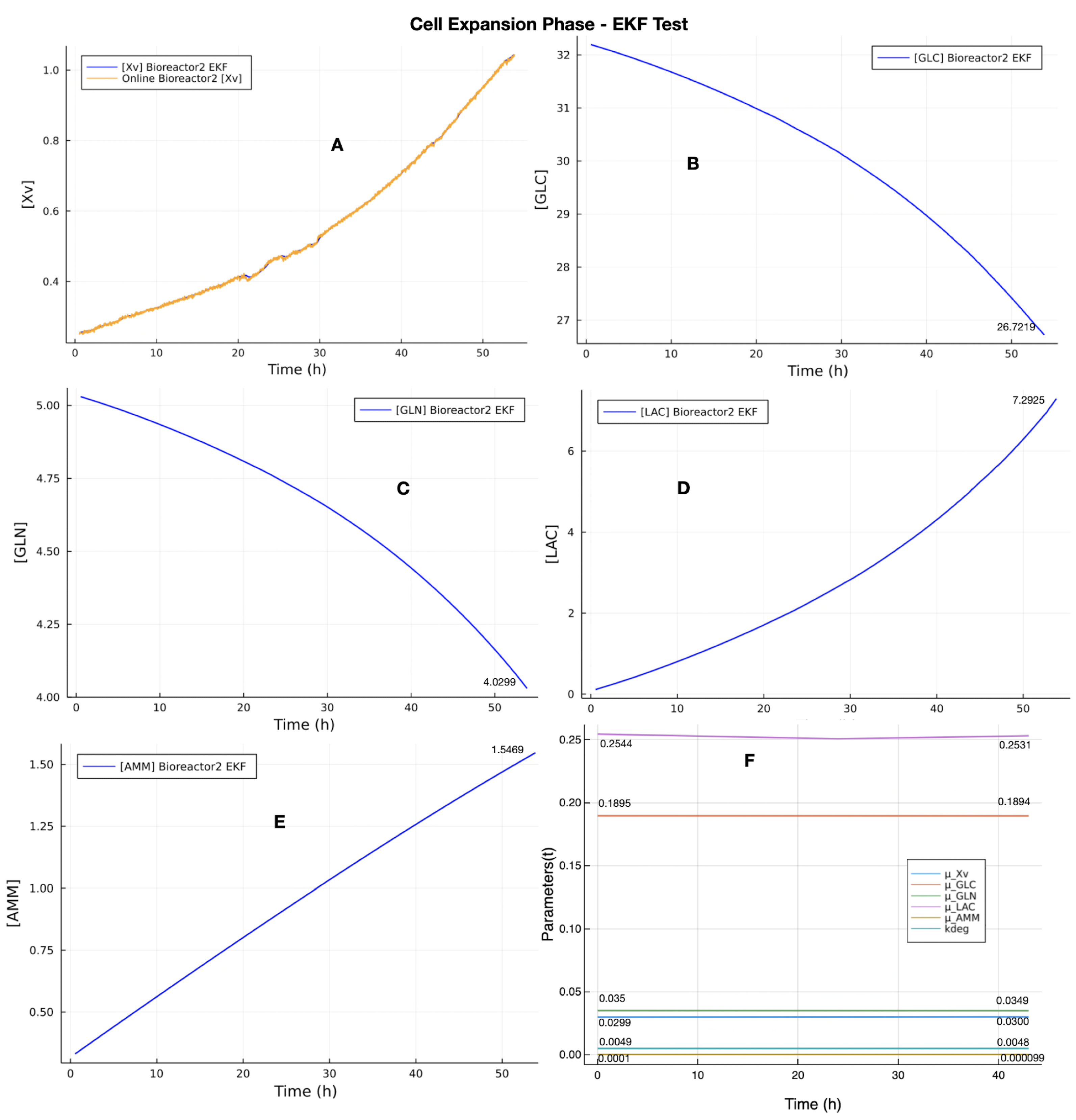
The first step in the EKF test was to estimate the state variables of CEP because we consider the final values estimated in CEP as the initial conditions of state variables that compose $\mathit{\psi }(t=0)$ to be used by EKF in VVPP. The EKF test was performed with the same EKF parameters (${\mathbf{P}}_{i,i}(t=0)$, ${\mathbf{Q}}_{i,i}$, and R) used in the calibration process (Table 5 and Table 6). However, the initial condition of state variables vector $\mathit{\psi }(t=0)$ in CEP was composed of state variables of the bioreactor 2 dataset (column 3 of

Table 7. Initial conditions of state variables for the EKF test with bioreactor 2.

State Variable	Name	Value in CEP	Value in VVPP 1
Xv	Viable cells	0.2512 × ${10}^6$ c/mL	1.0011 × ${10}^6$ c/mL
GLC	Glucose	32.19 mM	26.7219 mM
GLN	Glutamine	5.03 mM	4.0299 mM
LAC	Lactate	0.111 mM	7.2925 mM
AMM	Ammonium	0.33 mM	1.5469 mM
AAV	AAV viral titer	0 VG/mL	0 VG/mL

¹ These values are related to the final EKF estimation for CEP with bioreactor 2 dataset; see Figure 5.

) and the values of Bayesian UMKM parameters estimation (column 4 of Table 3). Figure 5 presents the results of EKF estimations in CEP. Plot A shows the online Xv measurements with noise (orange line) and EKF estimations following the exponential behavior of Xv (blue line). Plots B, C, D, and E present the final estimated values (last column of Table 7). The parameters estimation (plot F) presented the same behavior obtained by the calibration. It did not present the final values as being significantly different from the initial parameters. This is because the initial conditions of UMKM state variables in bioreactor 1 and 2 datasets are the same in CEP.

The EKF estimations for the VVPP were performed using the initial state variable vector $\mathit{\psi }(t=0)$ composed of the estimated concentrations of GLC, GLN, LAC, and AMM (last column in Table 7), the initial online measurement of Xv in VVPP as the initial concentration of Xv, and the values of Bayesian UMKM parameters estimation (column 6 of Table 3). The EKF results in VVPP are presented in Figure 6. Plot A presents the online measurements of Xv (orange line) with noises and the EKF estimation (blue line). The red line is UMKM estimation with the parameter µXv obtained from the bioreactor 1 dataset, which is the initial value of $\mathit{\psi }(t=0)$ in VVPP. Comparing UMKM and EKF estimation, we can see that bioreactor 1 and 2 datasets have different dynamics for Xv measurements, but the EKF followed the real dynamics of the bioreactor 2 dataset. Plots B, C, and D show the EKF estimation for GLC, LAC, and rAAV. All EKF estimations (blue lines) are near to the offline measurements (reference data) of these state variables (red points). On the other hand, the red lines show the UMKM estimations in VVPP using the parameters ${\mu }_{GLC},{\mu }_{LAC}$, and ${\mu }_{AAV}$ of column 6 of Table 3 without updates during the entire estimation process. The UMKM estimations were far from the offline measurements. These results were confirmed with the RMSE of the EKF and UMKM estimations with the offline measurements of the bioreactor 2 dataset; see

Table 8. RMSE values of the EKF and UMKM estimations regarding bioreactor 2 dataset in the EKF test.

State Variable	Name	RMSE of UMKM Estimation with Parameters Estimated by BI	RMSE of EKF Estimation
GLC	Glucose	2.931	0.778
LAC	Lactate	2.29	0.228
AAV	AAV viral titer	2.616	0.355

. The RMSE values of the EKF estimation are the lowest, resulting from the parameter estimation performed by EKF that updates the parameters ${\mu }_{GLC},{\mu }_{LAC}$, and ${\mu }_{AAV}$ of column 6 of Table 3 during the estimation process. The plot E shows the parameter estimation regarding VVPP performed in this test by the EKF. In this plot E, we can see that all state variables converged to a final value higher than the initial value. However, the parameters of GLC, LAC, and rAAV (${\mu }_{GLC},{\mu }_{LAC}$, and ${\mu }_{AAV}$) showed a significant difference compared to their initial parameter values. This is because these initial values were obtained from the bioreactor 1 dataset and the EKF updated them to the bioreactor 2 dataset, another cell culture regarding rAAV production.

4. Discussion

The main result of the evaluation came from the EKF test (Section 3.3). However, the EKF test depended on the results of the UMKM parameters estimation (Section 3.1) and the EKF calibration (Section 3.2) to be performed, as described in Section 2.6. The UMKM parameters estimation performed by NODE and Bayesian inference found congruent parameters values (Section 3.1). Besides these values being used as the initial condition in the state variables vector $\mathit{\psi }(t=0)$, they were also used in the EKF calibration to obtain the final values of EKF parameters ${\mathbf{P}}_{i,i}(t=0)$ and ${\mathbf{Q}}_{i,i}$ to be used in the EKF test. The results of the EKF test showed that the proposed EKF, with the process model (UMKM) depending only on the online viable cells (Xv) measurements, was able to estimate the other state variables of rAAV production, with values very close to the offline measurements. These results imply that the proposed EKF has solid potential to evolve into an online soft-sensor application and to be viewed as a low-cost and fast solution for monitoring rAAV production throughout the upstream process at the macroscale. This is because the offline/online measurement process of the state variables (viable cell density, metabolites, and rAAV viral titer ) used to generate the datasets required the use of multiple assays/devices to perform the measurements of all state variables (as described in Section 2.4.5 and Figure 2), whereas the proposed EKF requires only one (as described in Section 3.3 and Figure 1). The reason for this is that the Xv measurement (viable cells) will be an input to the EKF, which is then used to estimate all state variables of rAAV production. It can consequently reduce the costs of frequent sampling. Furthermore, the fact that EKF relies only on Xv measurements to estimate all state variables is a desirable step forward for online soft sensors since they are used to estimate state variables over time that are difficult to measure directly, or that can only be measured at a low sampling rate [18]. However, despite significant results achieved by the proposed EKF, it is important to point out that it has limitations and needs more tests and further improvements. The proposed approach cannot contribute to the understanding of the rAAV production mechanistic model and should be considered as a limitation. Furthermore, more tests and improvements should be considered to extend the proposed EKF to a stable soft-sensor application that is ready to be used in the industry. Three future research directions might be considered. The first direction is related to increasing the complexity of the mechanistic model. The UMKM and EKF had the same performance in estimating AMM, but they did not perform a prediction near the observed data properly. The main reason for this discrepancy is that the conversion between NH4+, NH3(aq), and NH3(g) is not considered in the model. The sparging of oxygen and constant air overlay flow would remove the NH3(g) so that the reaction equilibrium shifts to the direction of converting NH4+ to NH3(g), hence decreasing NH4+ at the end of process. This could be solved by introducing an AMM removal term to Equation (5) [35,52]. It is noteworthy that the trend of Xv during VVPP is not exponential. This may be because of transfection, nutrition limits (GLC and GLN), and toxic compound accumulation (LAC and AMM). Second, an additional improvement is estimating the parameters with other methods to confirm the convergence obtained. An option includes calibrating parameters outside the EKF calculation with an outer optimization routine [29]. Third, the proposed EKF needs validation with different datasets containing offline and online measurements of rAAV productions. The datasets used in this initial study allow us to test the proposed EKF, aiming to have a preliminary idea about its potential as an approach to monitoring the rAAV production using only the Xv measurements to estimate the state variables of rAAV production, but the datasets limit the final validation because of their small size and missing online and offline measurements.

5. Conclusions

The first step toward increasing rAAV viral titer productivity is to perform efficient monitoring with technology that will increase the speed and reduce the cost by automating tedious tasks. The present work was an initial study that proposed an EKF application to estimate state variables of rAAV production in different phases of the upstream process based only on online/offline measurements of Xv. The proposed EKF used an UMKM as a process model that models the upstream process (cell expansion and viral vector production kinetic models). The initial parameters of UMKM and EKF were estimated with Bayesian inference and updated during the EKF process. The development and evaluation of the proposed EKF were performed with three datasets (shake-flasks, bioreactor 1, and bioreactor 2 datasets), where the data were collected from the production of rAAV through the triple-plasmid transfection of HEK293SF-3F6 cells. The evaluation showed that the EKF used the online/offline Xv measurements and efficiently estimated the state variables (GLC, LAC, and rAAV). Our findings based on the main results of the evaluation (EKF test) are twofold: first, the proposed EKF indicates that it can reduce the number of devices for monitoring the state variables for rAAV production over the upstream process phase since it requires only one device to measure Xv. This contrasts with current approaches that require multiple assays/devices to monitor the rAAV production. Second, the proposed EKF can enable the online monitoring of the rAAV viral titer since all EKF estimations on the rAAV viral titer were performed in real-time using only online Xv measurements. These estimations allow for the monitoring of the rAAV viral titer every 1 min, in contrast with conventional approaches that can deliver a result on the rAAV viral titer productivity only after the entire process is completed, which can take one day after the production. The results obtained with the proposed EKF show the potential of the approach, which might be extended to a soft sensor or a model predictive control (MPC) application to enable the low-cost and fast monitoring of rAAV production. Our future works will focus on increasing the complexity of UMKM, testing other parameters estimation methods with EKF, and validating the EKF with more datasets.

References

1. Wang, D.; Tai, P.W.; Gao, G. Adeno-associated virus vector as a platform for gene therapy delivery. Nat. Rev. Drug Discov. 2019, 18, 358–378. [Google Scholar] [CrossRef] [PubMed]
2. Bulcha, J.T.; Wang, Y.; Ma, H.; Tai, P.W.; Gao, G. Viral vector platforms within the gene therapy landscape. Signal Transduct. Target. Ther. 2021, 6, 1–24. [Google Scholar] [CrossRef] [PubMed]
3. Naso, M.F.; Tomkowicz, B.; Perry, W.L.; Strohl, W.R. Adeno-associated virus (AAV) as a vector for gene therapy. BioDrugs 2017, 31, 317–334. [Google Scholar] [CrossRef] [Green Version]
4. Keeler, A.M.; Flotte, T.R. Recombinant adeno-associated virus gene therapy in light of Luxturna (and Zolgensma and Glybera): Where are we, and how did we get here? Annu. Rev. Virol. 2019, 6, 601–621. [Google Scholar] [CrossRef] [PubMed]
5. Srivastava, A.; Mallela, K.M.; Deorkar, N.; Brophy, G. Manufacturing challenges and rational formulation development for AAV viral vectors. J. Pharm. Sci. 2021, 110, 2609–2624. [Google Scholar] [CrossRef] [PubMed]
6. Food and Drug Administration. Guidance for Industry, PAT-A Framework for Innovative Pharmaceutical Development, Manufacturing and Quality Assurance. Available online: https://www.fda.gov/media/71012/download (accessed on 15 July 2022).
7. Gimpel, A.L.; Katsikis, G.; Sha, S.; Maloney, A.J.; Hong, M.S.; Nguyen, T.N.; Wolfrum, J.; Springs, S.L.; Sinskey, A.J.; Manalis, S.R.; et al. Analytical methods for process and product characterization of recombinant adeno-associated virus-based gene therapies. Mol.-Ther.-Methods Clin. Dev. 2021, 20, 740–754. [Google Scholar] [CrossRef] [PubMed]
8. Ohadi, K.; Aghamohseni, H.; Legge, R.L.; Budman, H.M. Fluorescence-based soft sensor for at situ monitoring of chinese hamster ovary cell cultures. Biotechnol. Bioeng. 2014, 111, 1577–1586. [Google Scholar] [CrossRef]
9. Claßen, J.; Graf, A.; Aupert, F.; Solle, D.; Höhse, M.; Scheper, T. A novel LED-based 2D-fluorescence spectroscopy system for in-line bioprocess monitoring of Chinese hamster ovary cell cultivations—Part II. Eng. Life Sci. 2019, 19, 341–351. [Google Scholar] [CrossRef] [Green Version]
10. Whelan, J.; Craven, S.; Glennon, B. In situ Raman spectroscopy for simultaneous monitoring of multiple process parameters in mammalian cell culture bioreactors. Biotechnol. Prog. 2012, 28, 1355–1362. [Google Scholar] [CrossRef]
11. Abu-Absi, N.R.; Kenty, B.M.; Cuellar, M.E.; Borys, M.C.; Sakhamuri, S.; Strachan, D.J.; Hausladen, M.C.; Li, Z.J. Real time monitoring of multiple parameters in mammalian cell culture bioreactors using an in-line Raman spectroscopy probe. Biotechnol. Bioeng. 2011, 108, 1215–1221. [Google Scholar] [CrossRef]
12. Berry, B.; Moretto, J.; Matthews, T.; Smelko, J.; Wiltberger, K. Cross-scale predictive modeling of CHO cell culture growth and metabolites using R aman spectroscopy and multivariate analysis. Biotechnol. Prog. 2015, 31, 566–577. [Google Scholar] [CrossRef] [PubMed]
13. Faassen, S.M.; Hitzmann, B. Fluorescence spectroscopy and chemometric modeling for bioprocess monitoring. Sensors 2015, 15, 10271–10291. [Google Scholar] [CrossRef] [PubMed] [Green Version]
14. Tsopanoglou, A.; del Val, I.J. Moving towards an era of hybrid modelling: Advantages and challenges of coupling mechanistic and data-driven models for upstream pharmaceutical bioprocesses. Curr. Opin. Chem. Eng. 2021, 32, 100691. [Google Scholar] [CrossRef]
15. Chhatre, S. Modelling approaches for bio-manufacturing operations. Meas. Monit. Model. Control. Bioprocesses 2012, 132, 85–107. [Google Scholar]
16. Udugama, I.A.; Lopez, P.C.; Gargalo, C.L.; Li, X.; Bayer, C.; Gernaey, K.V. Digital Twin in biomanufacturing: Challenges and opportunities towards its implementation. Syst. Microbiol. Biomanufacturing 2021, 1, 257–274. [Google Scholar] [CrossRef]
17. Luo, Y.; Kurian, V.; Ogunnaike, B.A. Bioprocess systems analysis, modeling, estimation, and control. Curr. Opin. Chem. Eng. 2021, 33, 100705. [Google Scholar] [CrossRef]
18. Reyes, S.J.; Durocher, Y.; Pham, P.L.; Henry, O. Modern Sensor Tools and Techniques for Monitoring, Controlling, and Improving Cell Culture Processes. Processes 2022, 10, 189. [Google Scholar] [CrossRef]
19. Koutinas, M.; Kiparissides, A.; Pistikopoulos, E.N.; Mantalaris, A. Bioprocess systems engineering: Transferring traditional process engineering principles to industrial biotechnology. Comput. Struct. Biotechnol. J. 2012, 3, e201210022. [Google Scholar] [CrossRef] [Green Version]
20. Kotidis, P.; Pappas, I.; Avraamidou, S.; Pistikopoulos, E.N.; Kontoravdi, C.; Papathanasiou, M.M. DigiGlyc: A hybrid tool for reactive scheduling in cell culture systems. Comput. Chem. Eng. 2021, 154, 107460. [Google Scholar] [CrossRef]
21. Narayanan, H.; Sokolov, M.; Morbidelli, M.; Butté, A. A new generation of predictive models: The added value of hybrid models for manufacturing processes of therapeutic proteins. Biotechnol. Bioeng. 2019, 116, 2540–2549. [Google Scholar] [CrossRef]
22. Narayanan, H.; Behle, L.; Luna, M.F.; Sokolov, M.; Guillén-Gosálbez, G.; Morbidelli, M.; Butté, A. Hybrid-EKF: Hybrid model coupled with extended Kalman filter for real-time monitoring and control of mammalian cell culture. Biotechnol. Bioeng. 2020, 117, 2703–2714. [Google Scholar] [CrossRef] [PubMed]
23. Fernandes-Platzgummer, A.; Badenes, S.M.; da Silva, C.L.; Cabral, J.M. Bioreactors for Stem Cell and Mammalian Cell Cultivation. Bioprocess. Technol. Prod. Biopharm. Bioprod. 2018, 131–173. [Google Scholar] [CrossRef]
24. Mears, L.; Stocks, S.M.; Albaek, M.O.; Sin, G.; Gernaey, K.V. Mechanistic fermentation models for process design, monitoring, and control. Trends Biotechnol. 2017, 35, 914–924. [Google Scholar] [CrossRef]
25. Nguyen, T.N.; Sha, S.; Hong, M.S.; Maloney, A.J.; Barone, P.W.; Neufeld, C.; Wolfrum, J.; Springs, S.L.; Sinskey, A.J.; Braatz, R.D. Mechanistic model for production of recombinant adeno-associated virus via triple transfection of HEK293 cells. Mol.-Ther.-Methods Clin. Dev. 2021, 21, 642–655. [Google Scholar] [CrossRef] [PubMed]
26. Zhang, D.; Del Rio-Chanona, E.A.; Petsagkourakis, P.; Wagner, J. Hybrid physics-based and data-driven modeling for bioprocess online simulation and optimization. Biotechnol. Bioeng. 2019, 116, 2919–2930. [Google Scholar] [CrossRef]
27. Kourti, T. 4.11-Multivariate Statistical Process Control and Process Control, Using Latent Variables. 2020. Comprehensive Chemometrics 2020, 275–303. [Google Scholar] [CrossRef]
28. Ohadi, K.; Legge, R.L.; Budman, H.M. Development of a soft-sensor based on multi-wavelength fluorescence spectroscopy and a dynamic metabolic model for monitoring mammalian cell cultures. Biotechnol. Bioeng. 2015, 112, 197–208. [Google Scholar] [CrossRef]
29. Yousefi-Darani, A.; Paquet-Durand, O.; Hitzmann, B. The Kalman Filter for the Supervision of Cultivation Processes. Springer International Publishing. 2020, 177, 95–125. Available online: https://link.springer.com/chapter/10.1007/10_2020_145 (accessed on 15 July 2022).
30. Paquet-Durand, O.; Zettel, V.; Yousefi-Darani, A.; Hitzmann, B. The Supervision of Dough Fermentation Using Image Analysis Complemented by a Continuous Discrete Extended Kalman Filter. Processes 2020, 8, 1669. [Google Scholar] [CrossRef]
31. Selişteanu, D.; Șendrescu, D.; Georgeanu, V.; Roman, M. Mammalian cell culture process for monoclonal antibody production: Nonlinear modelling and parameter estimation. Biomed Res. Int. 2015, 2015, 598721. [Google Scholar] [CrossRef] [Green Version]
32. Chahal, P.S.; Schulze, E.; Tran, R.; Montes, J.; Kamen, A.A. Production of adeno-associated virus (AAV) serotypes by transient transfection of HEK293 cell suspension cultures for gene delivery. J. Virol. Methods 2014, 196, 163–173. [Google Scholar] [CrossRef] [PubMed]
33. Kyriakopoulos, S.; Ang, K.S.; Lakshmanan, M.; Huang, Z.; Yoon, S.; Gunawan, R.; Lee, D.Y. Kinetic modeling of mammalian cell culture bioprocessing: The quest to advance biomanufacturing. Biotechnol. J. 2018, 13, 1700229. [Google Scholar] [CrossRef] [PubMed]
34. Tang, P.; Xu, J.; Louey, A.; Tan, Z.; Yongky, A.; Liang, S.; Li, Z.J.; Weng, Y.; Liu, S. Kinetic modeling of Chinese hamster ovary cell culture: Factors and principles. Crit. Rev. Biotechnol. 2020, 40, 265–281. [Google Scholar] [CrossRef] [PubMed]
35. Xing, Z.; Bishop, N.; Leister, K.; Li, Z.J. Modeling kinetics of a large-scale fed-batch CHO cell culture by Markov chain Monte Carlo method. Biotechnol. Prog. 2010, 26, 208–219. [Google Scholar] [CrossRef]
36. Jin, X.B.; Robert Jeremiah, R.J.; Su, T.L.; Bai, Y.T.; Kong, J.L. The new trend of state estimation: From model-driven to hybrid-driven methods. Sensors 2021, 21, 2085. [Google Scholar] [CrossRef]
37. Ji, Z.; Brown, M. Joint state and parameter estimation for biochemical dynamic pathways with iterative extended Kalman filter: Comparison with dual state and parameter estimation. Open Autom. Control. Syst. J. 2009, 2, 69–77. [Google Scholar] [CrossRef] [Green Version]
38. Brockwell, P. Time series analysis. Encycl. Stat. Behav. Sci. 2005. [CrossRef]
39. Dua, V.; Dua, P. A simultaneous approach for parameter estimation of a system of ordinary differential equations, using artificial neural network approximation. Ind. Eng. Chem. Res. 2012, 51, 1809–1814. [Google Scholar] [CrossRef]
40. Lee, K.; Parish, E.J. Parameterized neural ordinary differential equations: Applications to computational physics problems. Proc. R. Soc. A 2021, 477, 20210162. [Google Scholar] [CrossRef]
41. Rackauckas, C.; Innes, M.; Ma, Y.; Bettencourt, J.; White, L.; Dixit, V. Diffeqflux. jl-A julia library for neural differential equations. arXiv 2019, arXiv:1902.02376. [Google Scholar]
42. Xia, H.; Suliafu, V.; Ji, H.; Nguyen, T.; Bertozzi, A.; Osher, S.; Wang, B. Heavy ball neural ordinary differential equations. Adv. Neural Inf. Process. Syst. 2021, 34, 18646–18659. [Google Scholar]
43. Chen, R.T.; Rubanova, Y.; Bettencourt, J.; Duvenaud, D. Neural Ordinary Differential Equations. Advances in Neural Information Processing Systems. 2018, 31. Available online: https://arxiv.org/abs/1806.07366 (accessed on 15 July 2022).
44. Alahmadi, A.A.; Flegg, J.A.; Cochrane, D.G.; Drovandi, C.C.; Keith, J.M. A comparison of approximate versus exact techniques for Bayesian parameter inference in nonlinear ordinary differential equation models. R. Soc. Open Sci. 2020, 7, 191315. [Google Scholar] [CrossRef] [PubMed] [Green Version]
45. Ge, H.; Xu, K.; Ghahramani, Z. Turing: A language for flexible probabilistic inference. In Proceedings of the International Conference on Artificial Intelligence and Statistics, PMLR, Playa Blanca, Spain, 9–11 April 2018; pp. 1682–1690. [Google Scholar]
46. Dhadphale, J.M.; Unni, V.R.; Saha, A.; Sujith, R. Neural ODE to model and prognose thermoacoustic instability. Chaos Interdiscip. J. Nonlinear Sci. 2022, 32, 013131. [Google Scholar] [CrossRef] [PubMed]
47. Feldt, R. BlackBoxOptim.jl. Available online: https://github.com/robertfeldt/BlackBoxOptim.jl (accessed on 15 July 2022).
48. Shanmugavelayutham, G.J.C. Convergence analysis of differential evolution variants on unconstrained global optimization functions. arXiv 2011, arXiv:1105.1901. [Google Scholar]
49. Joshi, P.R.; Bernier, A.; Moço, P.D.; Schrag, J.; Chahal, P.S.; Kamen, A. Development of a scalable and robust AEX method for enriched rAAV preparations in genome-containing VCs of serotypes 5, 6, 8, and 9. Mol.-Ther.-Methods Clin. Dev. 2021, 21, 341–356. [Google Scholar] [CrossRef] [PubMed]
50. Judd, S.; Judd, C. Chapter 3–Design, operation and maintenance. In The MBR Book: Principles and Applications of Membrane Bioreactors for Water and Wastewater Treatment, 2nd ed.; Butterworth-Heinemann: Oxford, UK, 2011; pp. 55–207. [Google Scholar] [CrossRef]
51. O’Sullivan, M.; O’Sullivan, J. Reservoir modeling and simulation for geothermal resource In Book Geothermal Power Generation; Woodhead Publishing: Sawston, UK, 2016; pp. 165–199. [Google Scholar] [CrossRef]
52. Kornecki, M.; Strube, J. Accelerating biologics manufacturing by upstream process modelling. Processes 2019, 7, 166. [Google Scholar] [CrossRef]
Figure 1. EKF for rAAV production monitoring—the EKF performs a continuous estimation of UMKM state variables and parameters. The proposed EKF can use offline (b,c) and online (g) measurements of Xv collected from a bioreactor (a). The Xv measurements (the only measured state variable) are inputs (d) of EKF (e), which uses them to estimate the other state variables during rAAV production (f).
Processes 10 02180 g001
Figure 2. Current approach used for rAAV production monitoring: offline and online quantitative analysis. (a) The rAAV production was performed in shake-flasks and bioreactors. The offline measurements (b,c) were performed with the samples collected from these two environments and quantified in three different devices. Quantified state variables are Xv, Glc, Gln, Lac, Amm, and rAAV viral titer (d). The online measurement of Xv was performed in bioreactor 2 (e). The offline quantification of Xv, GLC, GLN, LAC, and AMM takes around 30 min for one set of data point, and the quantification of viral titer in rAAV production is carried out only at the end of production.
Processes 10 02180 g002
Figure 3. EKF calibration in CEP with bioreactor 1 dataset: the UMKM predictions were performed with parameters ( μ X v , μ G l c , μ G l n , μ L a c , μ A m m , k d e g , and μ A A V ) estimated by Bayesian inference (red lines in plots (AE)), and EKF estimation (blue lines in plots (AE)) was performed using these UMKM parameters as initial parameters, and were updated during the process. However, the final UMKM parameters found by EKF are not very different from those used as initial parameters obtained by Bayesian inference; see plot (F). The EKF and UMKM estimations were very similar.
Processes 10 02180 g003
Figure 4. EKF calibration in VVPP with bioreactor 1 dataset: the UMKM predictions were performed with parameters ( μ X v , μ G l c , μ G l n , μ L a c , μ A m m , k d e g , and μ A A V ) estimated by Bayesian inference (red lines in plots (AF)). EKF predictions (blue lines in plots (AF)) were performed using the parameters estimated by Bayesian inference as initial UMKM parameters since they were updated during the process. However, despite some fluctuations, the final parameters found are not very different from those used as initial parameters; see plot (G). The EKF was able to use the Xv measurement (with an outlier) and, similar to UMKM, estimate GLC, LAC, AMM, and rAAV.
Processes 10 02180 g004
Figure 5. EKF test with bioreactor 2 dataset for CEP-EKF estimation for the cell expansion phase of the upstream process. The Plot (A) shows the online Xv measurements with noise (orange line) and EKF estimations following the exponential behavior of Xv (blue line). The last values estimated by EKF in CEP are considered as the initial condition of state variables in VVPP (BE). The parameter estimation had some fluctuations regarding the LAC parameter, but the final parameters found are not very different from those used as initial parameters; see plot (F).
Processes 10 02180 g005
Figure 6. EKF test with bioreactor 2 dataset for VVPP: EKF estimation for the viral vector production phase of the upstream process. The UMKM predictions were performed with parameters estimated by Bayesian inference (red lines in plots (AD)) using bioreactor 1 dataset, and EKF estimation (blue lines in plots (AD)) was performed using these parameters as initial parameters. They were updated during the process; see Plot (E). The EKF was able to use the Xv measurement and performed estimation near to offline measurements of GLC, LAC, and rAAV.
Processes 10 02180 g006