Modeling the Transient Flow Behavior of Multi-Stage Fractured Horizontal Wells in the Inter-Salt Shale Oil Reservoir, Considering Stress Sensitivity

Abstract

Oil flow in inter-salt shale oil reservoirs is different from that of other oil fields due to its high salt content. Dissolution and diffusion occur when the salt minerals meet the water-based working fluid, resulting in drastic changes in the shale’s permeability. In addition, ignoring the stress-sensitive effect will cause significant errors in naturally fractured reservoirs for a large number of the natural fractures developed in shales. This study presents a transient pressure behavior model for a multi-stage fractured horizontal well (MFHW) in inter-salt shale oil reservoirs, considering the dissolution of salt and the stress sensitivity mentioned above. The analytical solution of our model was obtained by applying the methods of Pedrosa’s linearization, the perturbation technique and Laplace transformation. The transient pressure of a multi-stage fractured horizontal well in an inter-salt shale oil reservoir was obtained in real space by using the method of Stehfest’s numerical inversion. The bi-logarithmic-type curves thus obtained reflected the characteristics of the transient pressure behavior of a MFHW for the inter-salt shale oil reservoirs, and eight flow periods were recognized in the type curves. The effects of salt dissolution, stress sensitivity, the storativity ratio and other parameters on the type curves were analyzed thoroughly, which is of great significance for understanding the transient flow behavior of inter-salt shale oil reservoirs.

1. Introduction

An inter-salt shale oil reservoir is a set of shale oil reservoirs held by two sets of salt rock layers. The oil generated in inter-salt shales is easily stored in formation due to the separation of the upper and lower salt rock, and shows good exploration and development potential [1]. Due to the high salt content (23.88%) of the inter-salt shale oil reservoir, its development process is different from that of other oil fields. The permeability changes with effective pressure for a large number of natural fractures developed in shales. Therefore, a transient pressure model for oil flow in stress-sensitive inter-salt shale oil reservoirs is essential for evaluating underground fluid transport in such formations.

The inter-salt shale oil reservoir in Qianjiang Sag is rare both in China and abroad. The salt mineral content in the inter-salt shale oil reservoir is high, so the soluble amount of salt mineral is relatively high. Dissolution and diffusion occur when the salt minerals meet the water-based working fluid, and recrystallization occurs when the temperature and pressure change, resulting in drastic changes in the pores’ structure. Researchers have found through laboratory experiments that salt’s dissolution has an effect on shale’s permeability. Yang et al. observed the changes in the rock pores’ structure caused by the dissolution of salt through SEM images of the shale samples after soaking them in water [2]. Li et al. studied the influence of the salinity of injected water on the physical properties of inter-salt shale samples. They found that core permeability increased by 34.76% and 61.15% respectively after flooding with low-salinity water and ultra-pure water [3]. Zhang et al. found that the dissolution/precipitation of salt had a great influence on the seepage characteristics, and the damage by salt to the core permeability could reach more than 90% [4].

The stress-sensitive effect means that a decrease in pore pressure in the exploitation process of oil reservoirs increases the effective stress on the reservoir’s rock. The increase in overburden stress will lead to the elastic deformation and plastic deformation of the reservoir’s rock, making the formation compact [5,6]. The compaction will then reduce the effective pore diameter, resulting in a reduction in the permeability. The effect of stress sensitivity on a single porous medium has been studied by scholars [7,8,9] through experimental approaches, concluding that stress sensitivity has a greater effect on permeability than porosity. Vairogs et al. demonstrated experimentally that the reduction in permeability was proportionately greater in low-permeability than in high-permeability cores, and the fractures, and shale streaks exacerbated the reduction in permeability due to stress [10]. Scholars [11,12,13,14] have conducted a large number of studies on stress-sensitive reservoirs and found that not considering the stress-sensitive effect in low-permeability naturally fractured reservoirs will create large errors.

For a large number of natural fractures developed in shales, many researchers have studied seepage models of the gas or oil flow in dual-media reservoirs (which are composed of a matrix system and a fracture system [15]) based on the classical Warren–Root model [16]. Analytical models [17,18] and semi-analytical [19,20,21,22,23,24,25] models of fractured wells for shale gas reservoirs and tight gas/oil reservoirs have been studied by scholars. However, no study has provided an analytical model to study the transient pressure behavior of a fractured horizontal well for an inter-salt shale oil reservoir considering salt dissolution and the stress-sensitive effect. In this study, a transient pressure model of the MFHW in an inter-salt shale oil reservoir has been derived. The methods of Pedrosa’s linearization, the perturbation technique and Laplace transformation were used to find the solution of a line-sink considering the stress sensitivity in Laplace space. The pressure responses caused by the MFHW in the inter-salt shale oil reservoir based on the line-sink solution were obtained according to the superposition principle. The pressure response was then obtained by Stehfest’s numerical inversion algorithm. The results have been discussed here.

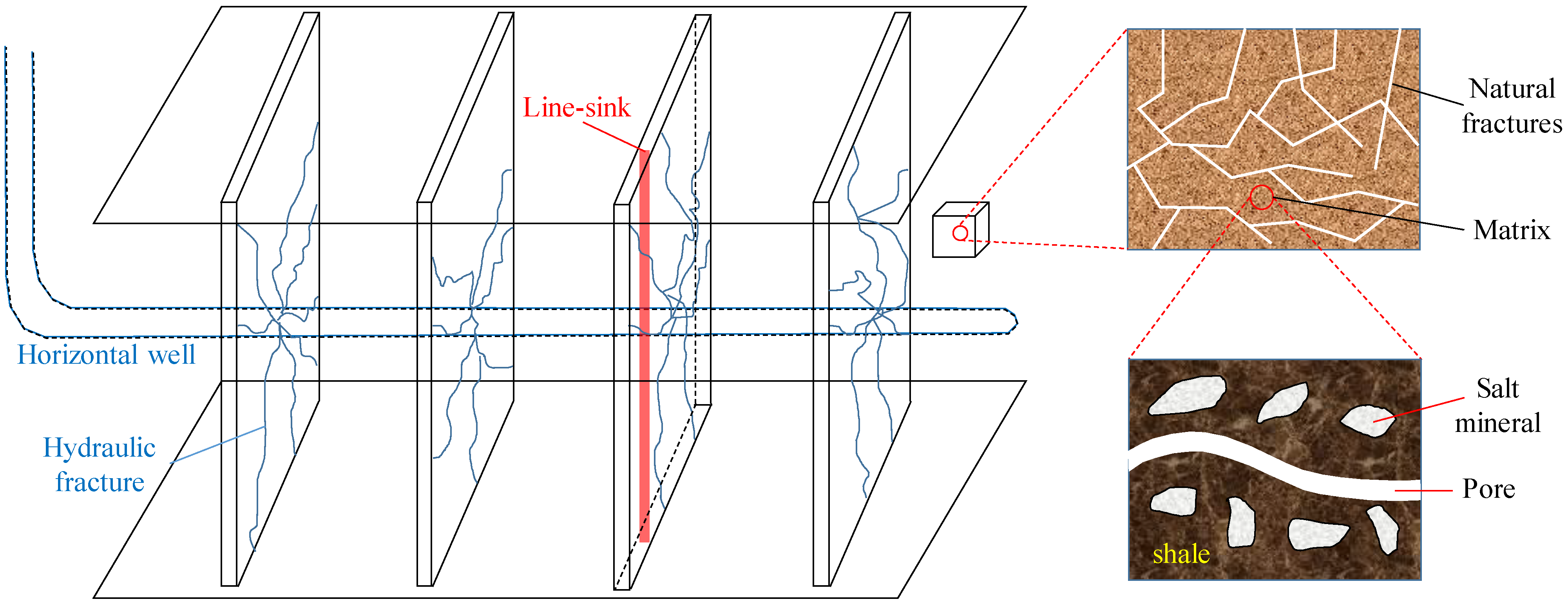
2. Physical Modeling

In this study, the inter-salt shale oil reservoir is composed of a matrix system and a fracture system, and the matrix system is segregated and surrounded by the fracture system. Given a multi-stage fractured horizontal well producing oil in an inter-salt shale oil reservoir (see Figure 1), oil flows from the matrix system to the fracture system and then flows to the fractured horizontal well. To make this mathematical model more tractable, the following assumptions and descriptions were made.

(1)

The reservoir is bounded by two parallel impermeable boundaries at the top and bottom, with an infinite lateral boundary. The reservoir’s thickness is h, and the initial formation pressure is p_i and is equal everywhere.

(2)

The inter-salt shale oil reservoir is assumed to be a dual-porosity medium, which is based on the Warren–Root model. The matrix porosity and fracture porosity are ϕ_m and ϕ_f, respectively, and the permeabilities are K_m and K_f. As K_f is much larger than K_m, pseudo-steady cross-flow occurs between these two systems.

(3)

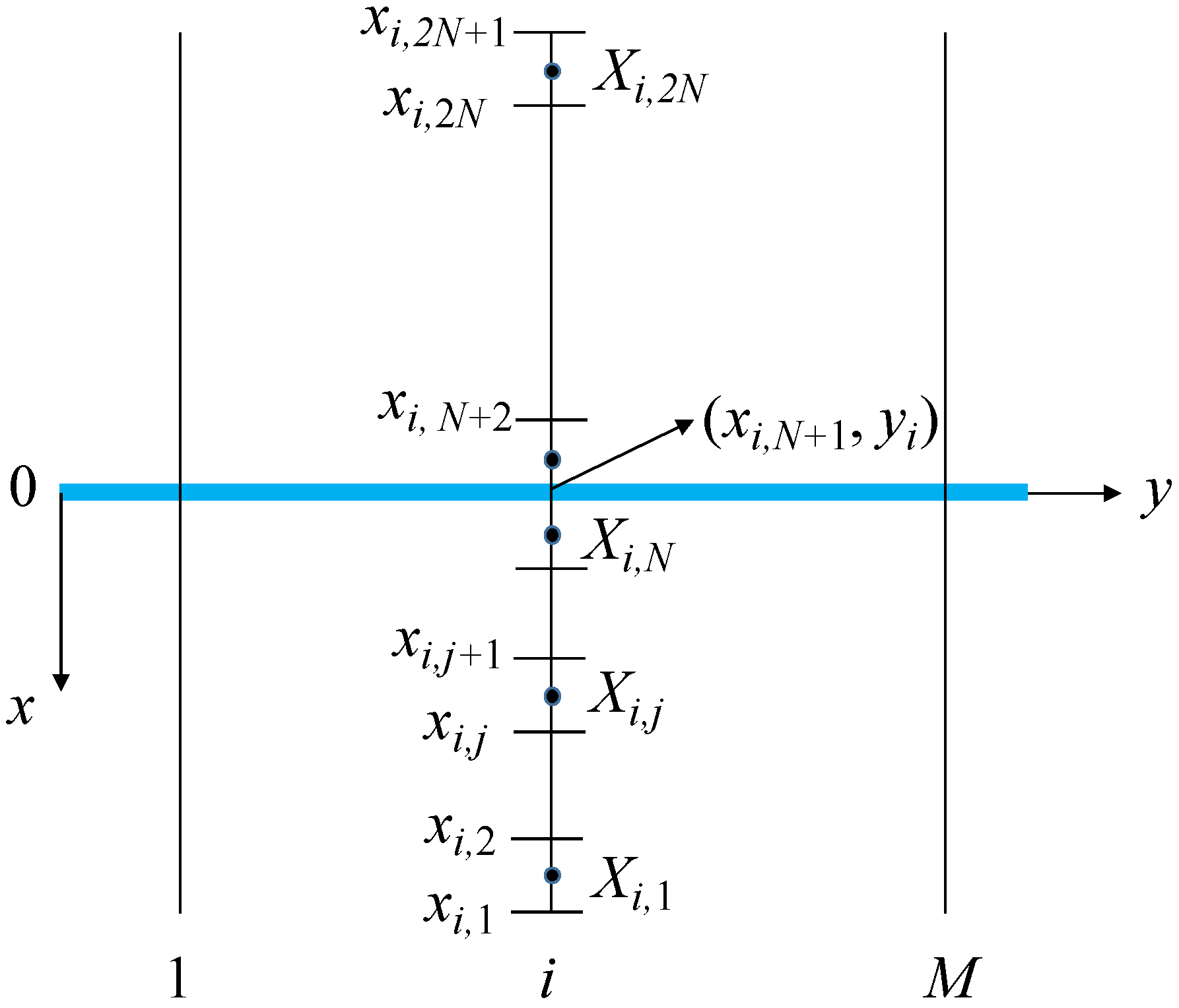
A fractured horizontal well can be located anywhere (represented by z_w) in the formation, with the horizontal section of the well parallel to the top and bottom boundaries. A total of M transverse fractures are formed after multi-stage fracturing.

(4)

The matrix permeability can be affected by the dissolution of salt. The fracture permeability is affected by the stress-sensitive effect, and oil flow in fracture system obeys Darcy’s law.

(5)

The single-phase oil is compressible with a constant viscosity and compression coefficient, but the wellbore storage effect and the skin effect are considered.

(6)

The oil flow in the inter-salt shale oil reservoir is at a constant reservoir temperature.

3. Mathematical Modeling

3.1. Mathematical Model of a Line-Sink in an Inter-Salt Shale Oil Reservoir

• Governing equations

In a cylindrical coordinate system, the shale reservoir is regarded as a dual-porosity model, and the mass conservation equation for oil flow in inter-salt shale oil reservoir can be written as follows.

For the matrix system:

$$\frac{\partial \left({\rho }_{\mathrm{m}}{\varphi }_{\mathrm{m}}\right)}{\partial t}+q_{\mathrm{ex}}=0$$

(1)

For the fracture system:

$$\frac{\partial \left({\rho }_{\mathrm{f}}{\varphi }_{\mathrm{f}}\right)}{\partial t}+\nabla \cdot \left(\rho v_{\mathrm{f}}\right)-q_{\mathrm{ex}}=0$$

(2)

The cross-flow equation can be written as:

$$q_{\mathrm{ex}}=\frac{\alpha K_{\mathrm{m}}{\rho }_0}{\mu }\left(p_{\mathrm{m}}-p_{\mathrm{f}}\right)$$

(3)

Considering the effect of salt dissolution on the matrix permeability, the permeability of the matrix system can be written as follows (see Appendix A)

$$K_{\mathrm{m}}=K_{\mathrm{mi}}-\beta \left(p_{\mathrm{i}}-p\right)=K_{\mathrm{mi}}-F$$

(4)

where F is the change in shale permeability after salt dissolution and can be calculated by Equation (4); it is treated as a constant in this model.

The motion equation of the fracture system, considering the effect of stress sensitivity, is written as [25,26]:

$$v_{\mathrm{fr}}=-\frac{K_{\mathrm{fi}}}{\mu }{\mathrm{e}}^{-\gamma \left(p_{\mathrm{i}}-p_{\mathrm{f}}\right)}\frac{\partial p_{\mathrm{f}}}{\partial r}$$

(5)

Since both porous media and fluids are compressible, equations of state (EOS) for porous media and elastic fluids need to be considered.

For shale rock:

$$\varphi ={\varphi }_0\left[1 + C_{\mathrm{p}}\left(p-p_0\right)\right]$$

(6)

For shale oil:

$$\rho ={\rho }_0\left[1 + C_{\mathrm{L}}\left(p-p_0\right)\right]$$

(7)

By substituting the equations above into the mass conservation Equations (1) and (2), the governing partial differential equations considering the effects of salt dissolution and stress sensitivity can be obtained.

$$\frac{1}{r}\frac{\partial }{\partial r}\left[r\frac{\partial p_{\mathrm{f}}}{\partial r}\right]+\gamma {\left(\frac{\partial p_{\mathrm{f}}}{\partial r}\right)}^2={\mathrm{e}}^{\gamma \left(p_{\mathrm{i}}-p_{\mathrm{f}}\right)}\left(\frac{{\varphi }_{\mathrm{f}}\mu c_{\mathrm{ft}}}{K_{\mathrm{fi}}}\frac{\partial p_{\mathrm{f}}}{\partial t}+\frac{{\varphi }_{\mathrm{m}}\mu c_{\mathrm{mt}}}{K_{\mathrm{fi}}}\frac{\partial p_{\mathrm{m}}}{\partial t}\right)$$

(8)

$${\varphi }_{\mathrm{m}}\mu c_{\mathrm{mt}}\frac{\partial p_{\mathrm{m}}}{\partial t}+\alpha \left(K_{\mathrm{mi}}-F\right)\left(p_{\mathrm{m}}-p_{\mathrm{f}}\right)=0$$

(9)

where the total compressibility coefficient C_t = (C_p + C_L), MPa⁻¹.

• Boundary conditions

The inner boundary condition is:

$$\underset{\epsilon \to 0}{\lim }{e}^{-\gamma \left(p_{\mathrm{i}}-p_{\mathrm{f}}\right)}{\left(r\frac{\partial p}{\partial r}\right)}_{r=\epsilon }=\frac{q\mu B}{2\pi K_{\mathrm{fi}}h}$$

(10)

The infinite lateral boundary condition is:

$${p_{\mathrm{f}}|}_{r\to \infty }={p_{\mathrm{m}}|}_{r\to \infty }=p_{\mathrm{i}}$$

(11)

• Initial conditions

$${p_{\mathrm{f}}|}_{t=0}={p_{\mathrm{m}}|}_{t=0}=p_{\mathrm{i}}$$

(12)

3.2. The Dimensionless Form of the Line-Sink Model

The mathematical model of the inter-salt shale oil reservoir was derived and solved in a dimensionless form in order to simplify the derivation and facilitate the comparison between different reservoirs.

With the definitions of dimensionless variables shown in

Table 1. Definitions of the dimensionless variables.

Dimensionless pressure	$p_{l\mathrm{D}}=\frac{2\pi K_{\mathrm{fi}}h\left(p_{\mathrm{i}} - p_l\right)}{q_{\mathrm{sc}}B\mu }$ (l = f, m)
Dimensionless time	$t_{\mathrm{D}}=\frac{K_{\mathrm{fi}}t}{\left({\varphi }_{\mathrm{f}}{c}_{\mathrm{ft}} + {\varphi }_{\mathrm{m}}{c}_{\mathrm{mt}}\right)\mu L^2}$
Dimensionless radius	$r_{\mathrm{D}}=\frac{r}{L}$
Storage coefficient	$\omega =\frac{{\varphi }_{\mathrm{f}}{c}_{\mathrm{ft}}}{{\varphi }_{\mathrm{f}}{c}_{\mathrm{ft}} + {\varphi }_{\mathrm{m}}{c}_{\mathrm{mt}}}$
Transfer coefficient	$\lambda =\alpha \frac{K_{\mathrm{mi}} - F}{K_{\mathrm{fi}}}{L}^2$
Dimensionless permeability modulus	${\gamma }_{\mathrm{D}}=\frac{q_{\mathrm{sc}}B\mu }{2\pi K_{\mathrm{fi}}h}\gamma$
Dimensionless wellbore storage coefficient	$C_{\mathrm{D}}=\frac{C}{\left({\varphi }_{\mathrm{f}}{C}_{\mathrm{ft}} + {\varphi }_{\mathrm{m}}{C}_{\mathrm{mt}}\right)h{L}^2}$
Dimensionless production rate	$q_{\mathrm{D}}=\frac{\tilde{q}L}{q_{\mathrm{sc}}}$

, the dimensionless forms of Equations (8)–(12) can be obtained as follows.

$$\mathrm{For} \mathrm{the} \mathrm{fracture}: \frac{{\partial }^2{p}_{\mathrm{fD}}}{\partial r_{\mathrm{D}}{}^2}+\frac{1}{r_{\mathrm{D}}}\frac{\partial p_{\mathrm{fD}}}{\partial r_{\mathrm{D}}}-{\gamma }_{\mathrm{D}}{\left(\frac{\partial p_{\mathrm{fD}}}{\partial r_{\mathrm{D}}}\right)}^2={\mathrm{e}}^{{\gamma }_{\mathrm{D}}{p}_{\mathrm{fD}}}\left[\omega \frac{\partial p_{\mathrm{fD}}}{\partial {\mathrm{t}}_{\mathrm{D}}}+\left(1-\omega \right)\frac{\partial p_{\mathrm{m}\mathrm{D}}}{\partial {\mathrm{t}}_{\mathrm{D}}}\right]$$

(13)

$$\mathrm{For} \mathrm{the} \mathrm{matrix}: \left(1-\omega \right)\frac{\partial p_{\mathrm{mD}}}{\partial {\mathrm{t}}_{\mathrm{D}}}+\lambda \left(p_{\mathrm{mD}}-p_{\mathrm{fD}}\right)=0$$

(14)

The inner boundary condition is:

$$\underset{{\epsilon }_{\mathrm{D}}\to 0}{\lim }{e}^{-{\gamma }_{\mathrm{mD}}{p}_{\mathrm{fD}}}{r}_{\mathrm{D}}{\frac{\partial p_{\mathrm{fD}}}{\partial r_{\mathrm{D}}}|}_{r_{\mathrm{D}}={\epsilon }_{\mathrm{D}}}=-1$$

(15)

The infinite lateral boundary condition is:

$${p_{\mathrm{fD}}|}_{r_{\mathrm{D}}\to \infty }={p_{\mathrm{mD}}|}_{r_{\mathrm{D}}\to \infty }=0$$

(16)

The initial condition is:

$${p_{\mathrm{fD}}|}_{t_{\mathrm{D}}=0}={p_{\mathrm{mD}}|}_{t_{\mathrm{D}}=0}=0$$

(17)

3.3. Solution of the Mathematical Line-Sink Model

3.3.1. Pedrosa’s Linearization

The inclusion of the stress sensitivity of natural fractures’ permeability makes the governing equation more complex and highly nonlinear, so it cannot directly be solved analytically. Pedrosa’s variable substitution can be applied to weaken the nonlinearity of the equation [27].

$$p_{\mathrm{fD}}\left(r_{\mathrm{D}},t_{\mathrm{D}}\right)=-\frac{1}{{\gamma }_{\mathrm{D}}}\ln \left[1-{\gamma }_{\mathrm{D}}{\xi }_{\mathrm{D}}\left(r_{\mathrm{D}},t_{\mathrm{D}}\right)\right]$$

(18)

where ξ_D(r_D, t_D) is an intermediate variable, also known as the perturbation deformation function.

Through Equation (18), Equations (13)–(17) become:

$$\begin{array}{l}\frac{{\partial }^2{\xi }_{\mathrm{D}}}{\partial r_{\mathrm{D}}{}^2}+\frac{1}{r_{\mathrm{D}}}\frac{\partial {\xi }_{\mathrm{D}}}{\partial r_{\mathrm{D}}}=\frac{1}{1-{\gamma }_{\mathrm{D}}{\xi }_{\mathrm{D}}}\omega \frac{\partial {\xi }_{\mathrm{D}}}{\partial t_{\mathrm{D}}}+\left(1-\omega \right)\frac{\partial p_{\mathrm{mD}}}{\partial t_{\mathrm{D}}}\\ \left(1-\omega \right)\frac{\partial p_{\mathrm{mD}}}{\partial t_{\mathrm{D}}}+\lambda \left[p_{\mathrm{mD}}+\frac{1}{{\gamma }_{\mathrm{D}}}\ln \left(1-{\gamma }_{\mathrm{D}}{\xi }_{\mathrm{D}}\right)\right]=0\\ \underset{{\epsilon }_{\mathrm{D}}\to 0}{\lim }{r}_{\mathrm{D}}{\frac{\partial {\xi }_{\mathrm{D}}}{\partial r_{\mathrm{D}}}|}_{r_{\mathrm{D}}={\epsilon }_{\mathrm{D}}}=-1\\ {{\xi }_{\mathrm{D}}|}_{r_{\mathrm{D}}\to \infty }={p_{\mathrm{mD}}|}_{r_{\mathrm{D}}\to \infty }=0\\ {{\xi }_{\mathrm{D}}|}_{t_{\mathrm{D}}=0}={p_{\mathrm{mD}}|}_{t_{\mathrm{D}}=0}=0\end{array}$$

(19)

3.3.2. Perturbation Technique

The perturbation technique can be applied to determine approximate analytical solutions for Equation (19), and it has proven to be an effective approach to solve such equations and showed the accuracy of the solution which has been widely applied in pressure transient analyses of stress-sensitive reservoirs by researchers [25,26,27,28,29]. According to the regular perturbation theory, the following terms can be expanded as a power series in the parameter 𝛾_D (dimensionless permeability modulus) [27,28]:

$${\xi }_{\mathrm{D}}={\xi }_{\mathrm{D}0}+{\gamma }_{\mathrm{D}}{\xi }_{\mathrm{D}1}+{\gamma }_{\mathrm{D}}^2{\xi }_{\mathrm{D}2}+\cdots$$

(20)

$$\frac{1}{1-{\gamma }_{\mathrm{D}}{\xi }_{\mathrm{D}}}=1 + {\gamma }_{\mathrm{D}}{\xi }_{\mathrm{D}}+{\gamma }_{\mathrm{D}}^2{\xi }_{\mathrm{D}}^2+\cdots$$

(21)

$$-\frac{1}{{\gamma }_{\mathrm{D}}}\ln \left(1-{\gamma }_{\mathrm{D}}{\xi }_{\mathrm{D}}\right)={\xi }_{\mathrm{D}}+\frac{1}{2}{\gamma }_{\mathrm{D}}{\xi }_{\mathrm{D}}^2+\cdots$$

(22)

Because the dimensionless permeability modulus is usually small (γ_D << 1), researchers [25,26,29] have suggested that the zero-order approximate solution can satisfy the requirements of engineering accuracy, so Equation (19) becomes:

$$\begin{array}{l}\frac{{\partial }^2{\xi }_{\mathrm{D}0}}{\partial r_{\mathrm{D}}{}^2}+\frac{1}{r_{\mathrm{D}}}\frac{\partial {\xi }_{\mathrm{D}0}}{\partial r_{\mathrm{D}}}=\omega \frac{\partial {\xi }_{\mathrm{D}0}}{\partial t_{\mathrm{D}}}+\left(1-\omega \right)\frac{\partial p_{\mathrm{mD}}}{\partial t_{\mathrm{D}}}\\ \left(1-\omega \right)\frac{\partial p_{m\mathrm{D}}}{\partial t_{\mathrm{D}}}+\lambda \left(p_{\mathrm{mD}}-{\xi }_{\mathrm{D}0}\right)=0\\ \underset{{\epsilon }_{\mathrm{D}}\to 0}{\lim }{r}_{\mathrm{D}}{\frac{\partial {\xi }_{\mathrm{D}0}}{\partial r_{\mathrm{D}}}|}_{r_{\mathrm{D}}={\epsilon }_{\mathrm{D}}}=-1\\ {{\xi }_{\mathrm{D}0}|}_{t_{\mathrm{D}}=0}={p_{\mathrm{mD}}|}_{t_{\mathrm{D}}=0}=0\\ {{\xi }_{\mathrm{D}0}|}_{r_{\mathrm{D}}\to \infty }={p_{\mathrm{mD}}|}_{r_{\mathrm{D}}\to \infty }=0\end{array}$$

(23)

Equation (23) is the linearized dimensionless line-sink model in a dual-porosity inter-salt shale oil reservoir, considering the effects of salt dissolution and stress sensitivity.

3.3.3. Laplace Transformation

Here, we introduce the following Laplace transformation

$$\overline{{\xi }_{\mathrm{D}0}}={\displaystyle {\int }_0^{+\infty }{\xi }_{\mathrm{D}0}{\mathrm{e}}^{-s{t}_{\mathrm{D}}}}\mathrm{d}t$$

(24)

where s is the Laplace transformation variable.

The Laplace transform is applied to the model in Equation (23) with respect to t_D, so Equation (23) can be written as:

$$\frac{{\partial }^2\overline{{\xi }_{\mathrm{D}0}}}{\partial r_{\mathrm{D}}{}^2}+\frac{1}{r_{\mathrm{D}}}\frac{\partial \overline{{\xi }_{\mathrm{D}0}}}{\partial r_{\mathrm{D}}}=\omega s\overline{{\xi }_{\mathrm{D}0}}+\left(1-\omega \right)s\overline{p_{\mathrm{mD}}}$$

(25)

$$\overline{p_{\mathrm{mD}}}=\frac{\lambda }{\lambda +\left(1-\omega \right)s}\overline{{\xi }_{\mathrm{D}0}}$$

(26)

$$\underset{{\epsilon }_{\mathrm{D}}\to 0}{\lim }{r}_{\mathrm{D}}{\frac{\partial \overline{{\xi }_{\mathrm{D}0}}}{\partial r_{\mathrm{D}}}|}_{r_{\mathrm{D}}={\epsilon }_{\mathrm{D}}}=-\frac{1}{s}$$

(27)

$${\overline{{\xi }_{\mathrm{D}0}}|}_{r_{\mathrm{D}}\to \infty }={\overline{p_{\mathrm{mD}}}|}_{r_{\mathrm{D}}\to \infty }=0$$

(28)

Let $u=\frac{\lambda +s\omega \left(1-\omega \right)}{\lambda +\left(1-\omega \right)s}s$, so Equation (25) can be written as:

$$\frac{{\partial }^2\overline{{\xi }_{\mathrm{D}0}}}{\partial r_{\mathrm{D}}^2}+\frac{1}{r_{\mathrm{D}}}\frac{\partial \overline{{\xi }_{\mathrm{D}0}}}{\partial r_{\mathrm{D}}}=u\overline{{\xi }_{\mathrm{D}0}}$$

(29)

The general solution of Equation (29) is

$$\overline{{\xi }_{\mathrm{D}0}}=A{I}_0\left(r_{\mathrm{D}}\sqrt{u}\right)+B{K}_0\left(r_{\mathrm{D}}\sqrt{u}\right)$$

(30)

where A and B are constants, and I₀ and K₀ are the Bessel function.

By substituting Equation (30) into the inter boundary condition, the following equation can be obtained:

$$\underset{{\epsilon }_{\mathrm{D}}\to 0}{\lim }{r}_{\mathrm{D}}{\sqrt{u}\left[A{I}_1\left(r_{\mathrm{D}}\sqrt{u}\right)-B{K}_1\left(r_{\mathrm{D}}\sqrt{u}\right)\right]|}_{r_{\mathrm{D}}={\epsilon }_{\mathrm{D}}}=-\frac{1}{s}$$

(31)

According to the properties of Bessel’s function, which are $\underset{x\to 0}{\lim }x{I}_1\left(x\right)\to 0$ and $\underset{x\to 0}{\lim }x{K}_1\left(x\right)\to 1$, we can obtain:

$$B=\frac{1}{s}$$

(32)

Substituting Equation (30) into the infinite outer boundary condition and the properties of Bessel’s function, which are $\underset{x\to \infty }{\lim }{I}_0\left(x\right)\to \infty$ and $\underset{x\to \infty }{\lim }{K}_0\left(x\right)\to 0$, we can obtain:

$$A=0$$

(33)

Therefore, we can obtain the line-sink solution of the dual-porosity model for an inter-salt shale oil reservoir, considering the stress sensitivity:

$$\overline{{\xi }_{\mathrm{D}0}}=\frac{1}{s}{K}_0\left(r_{\mathrm{D}}\sqrt{u}\right)$$

(34)

As mentioned above, the zero-order perturbation solution is sufficient for approximating the exact solution of Equation (19), so we can have:

$$\overline{{\xi }_{\mathrm{D}}}\approx \overline{{\xi }_{\mathrm{D}0}}=\frac{1}{s}{K}_0\left(r_{\mathrm{D}}\sqrt{u}\right)$$

(35)

When the line-sink is located at (x_w,y_w), r_D can be calculated by

$$r_{\mathrm{D}}=\sqrt{{\left(x_{\mathrm{D}}-x_{\mathrm{wD}}\right)}^2+{\left(y_{\mathrm{D}}-y_{\mathrm{wD}}\right)}^2}$$

(36)

where:

$$x_{\mathrm{D}}=\frac{x}{L}, y_{\mathrm{D}}=\frac{y}{L}, x_{\mathrm{wD}}=\frac{x_{\mathrm{w}}}{L}, y_{\mathrm{wD}}=\frac{y_{\mathrm{w}}}{L}$$

(37)

3.4. Pressure Responses of the MFHW in an Inter-Salt Shale Oil Reservoir

By applying the superposition principle, the pressure responses caused by the multistage fractured horizontal well in an inter-salt shale oil reservoir, based on the line-sink solution, can be obtained.

Figure 2 shows the schematic of a MFHW with M multiple hydraulic fractures. We assumed that the hydraulic fractures penetrated the entire reservoir, and the width of fractures was ignored. The horizontal wellbore is parallel to the y-axis, and the hydraulic fracture surface is perpendicular to the y-axis. The hydraulic fractures may be equally spaced or non-equally spaced, that is, the spacing between fractures (△L_i, i = 1, 2, ···, M−1) may be equal or unequal. Considering that the length of the hydraulic fractures may be different, we assumed that the length of the right wing and the left wing of the hydraulic fracture were L_fRi and L_fLi, respectively.

In order to obtain the pressure responses caused by multiple fractures based on the line-sink solution, it was necessary to discretize multiple fractures. As shown in Figure 2, the left wing and right wing of each hydraulic fracture are equally discretized into N segments, so each hydraulic fracture is discretized into 2N segments. Therefore, the coordinate of the midpoint of the jth segment on the ith fracture is denoted as (X_{i j}, Y_{i j}), and the coordinates of the endpoint are denoted as (x_{i j}, y_{i j}) and (x_{i j+1}, y_{i j+1}).

As shown in Figure 2, the coordinates of the endpoints of discrete segments can be calculated by:

$$\begin{array}{c}\{\begin{array}{l}{x}_{ij}=-\frac{N - j + 1}{N}{L}_{fLi}\\ y_{ij}=y_i\end{array}{ , }^{}1\le j\le N\\ \{\begin{array}{l}{x}_{ij}=-\frac{N - j + 1}{N}{L}_{fRi}\\ y_{ij}=y_i\end{array}{ , }^{}N+1\le j\le 2N\end{array}$$

(38)

The coordinate of the midpoint of each segment can be calculated by:

$$\begin{array}{c}\{\begin{array}{l}{X}_{ij}=-\frac{2N - 2j + 1}{2N}{L}_{fLi}\\ Y_{ij}=y_i\end{array} ,{{\displaystyle }}^{}1\le j\le N\\ \{\begin{array}{l}{X}_{ij}=-\frac{2N - 2j + 1}{2N}{L}_{fRi}\\ Y_{ij}=y_i\end{array} ,{{\displaystyle }}^{}N+1\le j\le 2N\end{array}$$

(39)

Because the flux strength along the fracture’s length is different, the flux density per unit of length q_i,j at different discrete segments is different. We assumed that the flux density was q_i,j for different discrete segments. Therefore, the pressure response caused by the discrete segment (i, j) at any location (x_D, y_D) in the inter-salt shale oil reservoir can be obtained by integrating the line-sink solution along the discrete segment:

$${\overline{\xi }}_{\mathrm{D}i,j}(x_{\mathrm{D}},y_{\mathrm{D}})=\frac{{\overline{q}}_{i,j}}{q_{\mathrm{sc}}}{\displaystyle \underset{x_{i,j}}{\overset{x_{i,j+1}}{\int }}{K}_0\left(\sqrt{u}\sqrt{{\left(x_{\mathrm{D}}-x_{\mathrm{wD}}\right)}^2+{\left(y_{\mathrm{D}}-y_{\mathrm{wD}}\right)}^2}\right)d{x}_{\mathrm{w}}}$$

(40)

According to the definitions of x_D and x_wD, Equation (40) can be written as:

$${\overline{\xi }}_{\mathrm{D}i,j}(x_{\mathrm{D}},y_{\mathrm{D}})=\frac{{\overline{q}}_{i,j}L}{q_{\mathrm{sc}}}{\displaystyle \underset{x_{\mathrm{D}i,j}}{\overset{x_{\mathrm{D}i,j+1}}{\int }}{K}_0\left(\sqrt{u}\sqrt{{\left(x_{\mathrm{D}}-x_{\mathrm{wD}}\right)}^2+{\left(y_{\mathrm{D}}-y_{\mathrm{wD}}\right)}^2}\right)d{x}_{\mathrm{wD}}}$$

(41)

The dimensionless flux per unit of length is defined as:

$$q_{\mathrm{D}i,j}=\frac{q_{i,j}L}{q_{\mathrm{sc}}}$$

(42)

Equation (41) can be written as:

$${\overline{\xi }}_{\mathrm{D}i,j}(x_{\mathrm{D}},y_{\mathrm{D}})={\overline{q}}_{\mathrm{D}i,j}{\displaystyle \underset{x_{\mathrm{D}i,j}}{\overset{x_{\mathrm{D}i,j+1}}{\int }}{K}_0\left(\sqrt{u}\sqrt{{\left(x_{\mathrm{D}}-x_{\mathrm{wD}}\right)}^2+{\left(y_{\mathrm{D}}-y_{\mathrm{wD}}\right)}^2}\right)d{x}_{\mathrm{wD}}}$$

(43)

According to the superposition principle, the pressure response at (x_D, y_D) caused by 2N × M segments on m hydraulic fractures can be obtained as:

$${\overline{\xi }}_{\mathrm{D}}(x_{\mathrm{D}},y_{\mathrm{D}})={\displaystyle \sum _{i=1}^M{\displaystyle \sum _{j=1}^{2N}{\overline{\xi }}_{\mathrm{D}i,j}\left(x_{\mathrm{D}},y_{\mathrm{D}}\right)}}$$

(44)

Thus, we can obtain the pressure response at the midpoint of each discrete segment (X_Dk,v, Y_Dk,v) as:

$${\overline{\xi }}_{\mathrm{D}}\left(x_{\mathrm{D}k,v},y_{\mathrm{D}k,v}\right)={\displaystyle \sum _{i=1}^M{\displaystyle \sum _{j=1}^{2N}{\overline{\xi }}_{\mathrm{D}i,j}\left(x_{\mathrm{D}k,v},y_{\mathrm{D}k,v}\right)}}$$

(45)

The pressure in the horizontal wellbore is equal to the pressure in each discrete segment of the hydraulic fractures, since the hydraulic fractures are assumed to be infinitely conductive. Therefore, the dimensionless pressure of the horizontal wellbore can be expressed as:

$${\overline{\xi }}_{\mathrm{wDN}}={\displaystyle \sum _{i=1}^M{\displaystyle \sum _{j=1}^{2N}{\overline{\xi }}_{\mathrm{D}i,j}\left(X_{\mathrm{D}k,v},X_{\mathrm{D}k,v}\right)}}$$

(46)

M × 2N equations can be obtained by rewriting Equation (46) for all discrete segments (k = 1, 2,…,M; v = 1, 2,…,2N). There are M × 2N + 1 unknowns in these M × 2N equations, so the constant total flow rate is written as:

$${\displaystyle \sum _{i=1}^M{\displaystyle \sum _{j=1}^{2N}\left[{\tilde{q}}_{i,j}\left(x_{i,j+1}-x_{i,j}\right)\right]=q_{\mathrm{sc}}}}$$

(47)

By taking the Laplace transform of Equation (47), we can obtain the following:

$${\displaystyle \sum _{i=1}^M{\displaystyle \sum _{j=1}^{2N}\left[{\overline{q}}_{\mathrm{D}i,j}\left(x_{\mathrm{D}i,j+1}-x_{\mathrm{D}i,j}\right)\right]=\frac{1}{s}}}$$

(48)

Therefore, Equations (47) and (48) represent a system of (M × 2N + 1) equations relating (M × 2N + 1) unknowns, which can be solved by the Gauss–Jordan reduction method or the Gaussian elimination method.

The effects of the wellbore’s storage and skin can be considered in the bottom-hole pressure response according to van Everdingen [30]:

$${\overline{\xi }}_{\mathrm{wD}}=\frac{s{\overline{\xi }}_{\mathrm{wDN}}+S}{s+C_D{s}^2\left(s{\overline{\xi }}_{\mathrm{wDN}}+S\right)}$$

(49)

In Equation (49), ${\overline{\xi }}_{\mathrm{wD}}$ is the bottom-hole pressure response in the Laplace domain, and the pressure response ξ_wD in the real time domain can be obtained by Stehfest’s numerical inversion algorithm [31]. The bottom-hole pressure response of multistage fractured horizontal wells in an inter-salt shale oil reservoir, considering the salt dissolution and stress sensitivity, can be obtained by the following equation:

$$p_{\mathrm{wD}}=-\frac{1}{{\gamma }_{\mathrm{D}}}\ln \left[1-{\gamma }_{\mathrm{D}}{\xi }_{\mathrm{wD}}\right]$$

(50)

4. Results and Discussion

The type curves of transient pressure can reflect the properties of underground reservoirs, and have been applied by many researchers [32,33,34,35]. The basic parameters needed for simulation are shown in

Table 2. Reservoir parameters needed for simulation.

Parameters	Symbols	Values	Units
Formation thickness	h	50	m
Formation pressure	pi	2.34 × 107	Pa
Permeability modulus	γ	0.12	MPa−1
Matrix porosity	ϕm	0.10	dimensionless
Matrix permeability	Km	2.4 × 10−19	m2
Fracture porosity	ϕf	0.039	dimensionless
Fracture permeability	Kf	2.0 × 10−13	m2
Oil viscosity	μ	2.95 × 10−3	Pa·s
Matrix compressibility	cmt	6.2 × 10−11	1/Pa
Fracture compressibility	cft	4.3 × 10−9	1/Pa
Half-length of the hydraulic fracture	Xf	230	m

, and the type curves of the transient pressure behavior of a MFHW for the inter-salt shale oil reservoir are presented in Section 4.1.

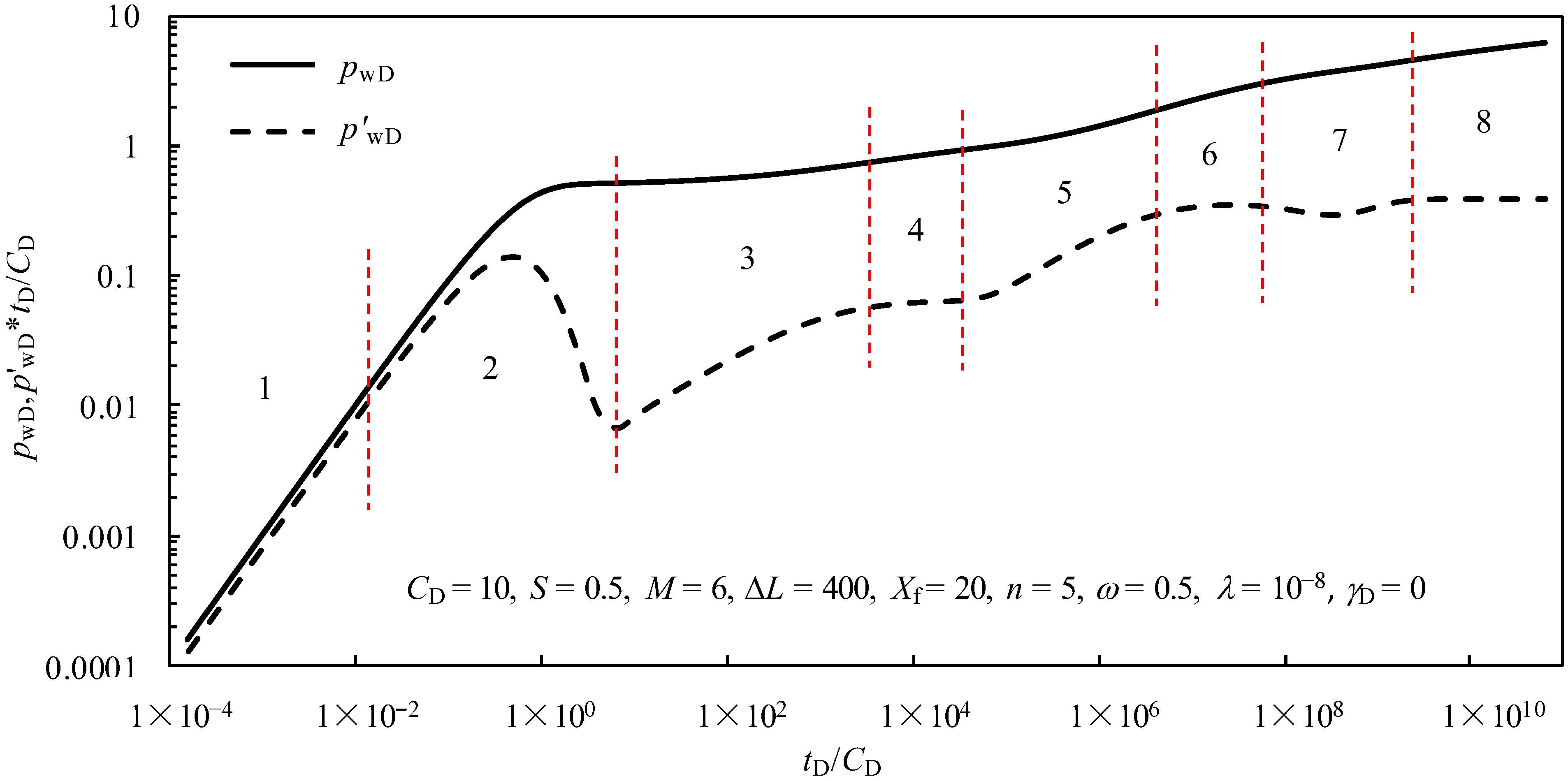
4.1. Behaviorial Analysis of Transient Pressure

Figure 3 presents the dimensionless pressure curve and the corresponding pressure derivative curve of a MFHW in an inter-salt shale oil reservoir with consideration of the salt dissolution and stress sensitivity of natural fractures. The following eight main transient flow periods can be recognized.

Period 1: The pure wellbore storage regime. In this stage, both the pressure curve and its derivative curve show an upward straight line with a slope of 1, which is controlled by the oil stored in the wellbore.

Period 2: The transition flow period. The shape of the pressure derivative curve resembles a hump, which is controlled by the skin factor S.

Period 3: The linear flow period of hydraulic fractures. The pressure derivative curve is an upward straight line with a slope of 0.5. In this flow period, the shale oil stored in natural fractures flows linearly in the direction perpendicular to the plane of the hydraulic fracture.

Period 4: The radial flow period of hydraulic fractures. The pressure derivative curve is a nearly horizontal line with a value of 1/2M. In this period, the shale oil stored in the natural fracture flows radially towards the hydraulic fracture.

Period 5: The linear flow period of natural fractures. The pressure derivative curve is a straight line with a slope of about 1/2. In this period, the hydraulic fractures and the horizontal wellbore are taken as a whole, and the formation fluid flows linearly, perpendicular to the horizontal wellbore.

Period 6: The radial flow period of natural fractures. The pressure derivative curve is a horizontal line with a value of 0.5, which reflects the radial flow of the natural fracture system.

Period 7: The interporosity flow period. This period is when the oil stored in the matrix flows into the natural fracture system. The most obvious feature is the dip in the pressure derivative curve.

Period 8: The late-time pseudoradial flow period of the entire system. In this period, the pressure drop spreads far from the wellbore in the reservoir, and a horizontal line with a value of 0.5 reappears in the pressure derivative curve.

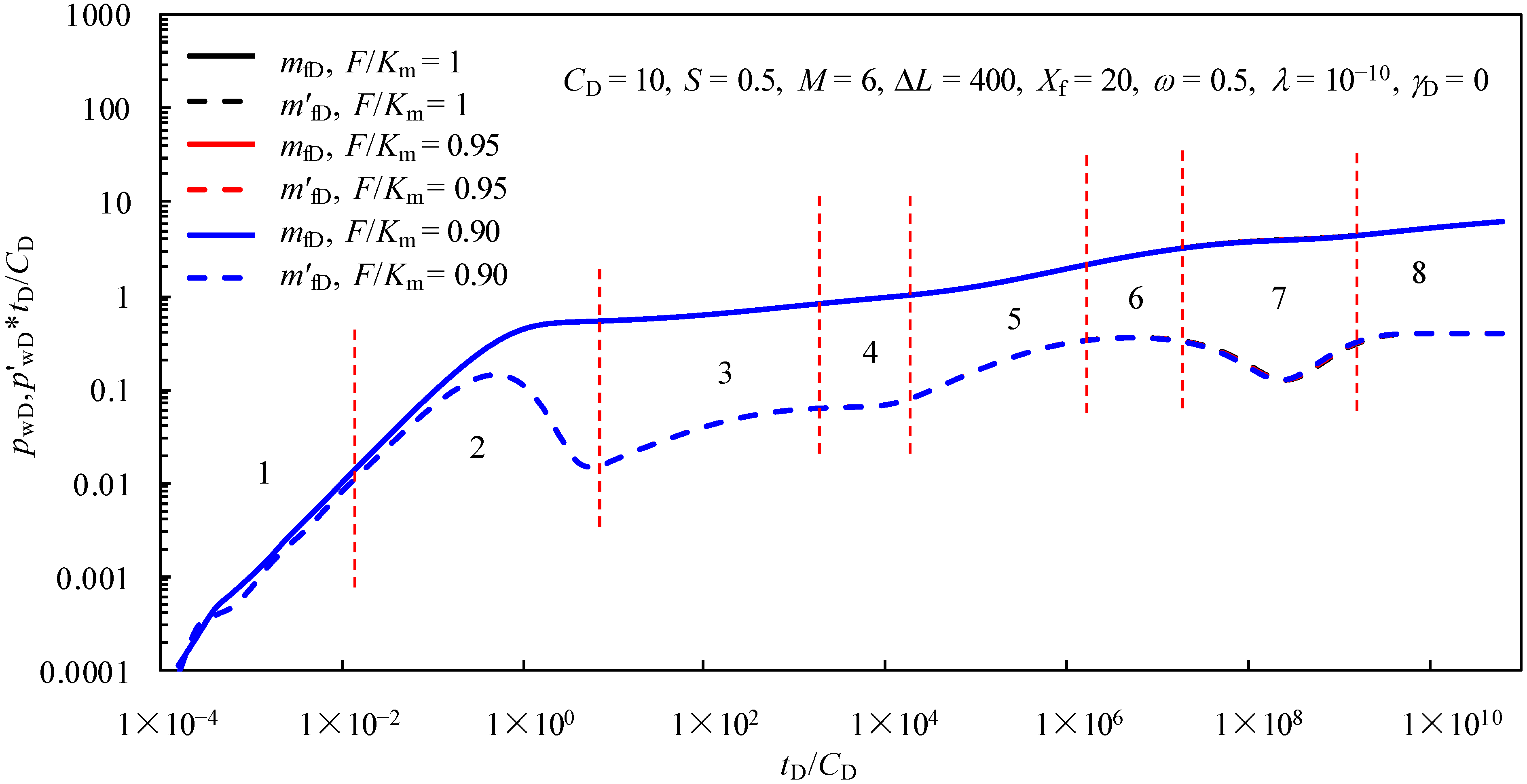
4.2. Effect of Salt Dissolution

Figure 4 presents the effect of salt dissolution on the dimensionless pressure and pressure derivative curves of a MFHW in an inter-salt shale oil reservoir. According to the experimental results of the effect of salt dissolution on the shale’s permeability, the permeability decreased by 5.06% when the average pressure dropped from 22.5 MPa to 7.5 MPa. The mathematical relationship obtained by the experiment was entered into our model, and the transient pressure curves influenced by the salt dissolution of the fractured horizontal well in an inter-salt shale oil reservoir were drawn. It can be seen in the figure that the effect of salt dissolution on the transient pressure curve of the fractured horizontal well in the shale oil reservoir was negligible.

4.3. Effect of Stress Sensitivity

Figure 5 shows the effect of stress sensitivity on the dimensionless pressure and the pressure derivative curves. Starting from the radial flow period of natural fractures (Period 6), the effect of the stress sensitivity of the fracture system on the pressure derivative curves becomes apparent. With an increase in the dimensionless permeability modulus, the dimensionless pressure and the pressure derivative curves gradually begin to turn upward in the last three flow periods. The greater the value of the dimensionless permeability modulus, the stronger the stress sensitivity, and the more serious the damage to the reservoir. Therefore, it is more difficult for the shale oil to flow, and more drawdown pressure is required.

4.4. Effect of the Storativity Ratio

Figure 6 shows the effect of the storativity ratio on the dimensionless pressure and pressure derivative curves. It can be seen from the figure that the storativity ratio affects the interporosity flow period (Period 7) of a typical curve and also affects the linear flow period (Period 3). The higher the value of ω is, the more oil is stored in the natural fracture system. Therefore, the natural fracture system can provide more oil to the hydraulic fractures, so the pressure derivative curve is deeper in Period 3. When the ω is smaller, the matrix system supplies more oil to the natural fracture system, so the dip is wider and deeper in Period 7.

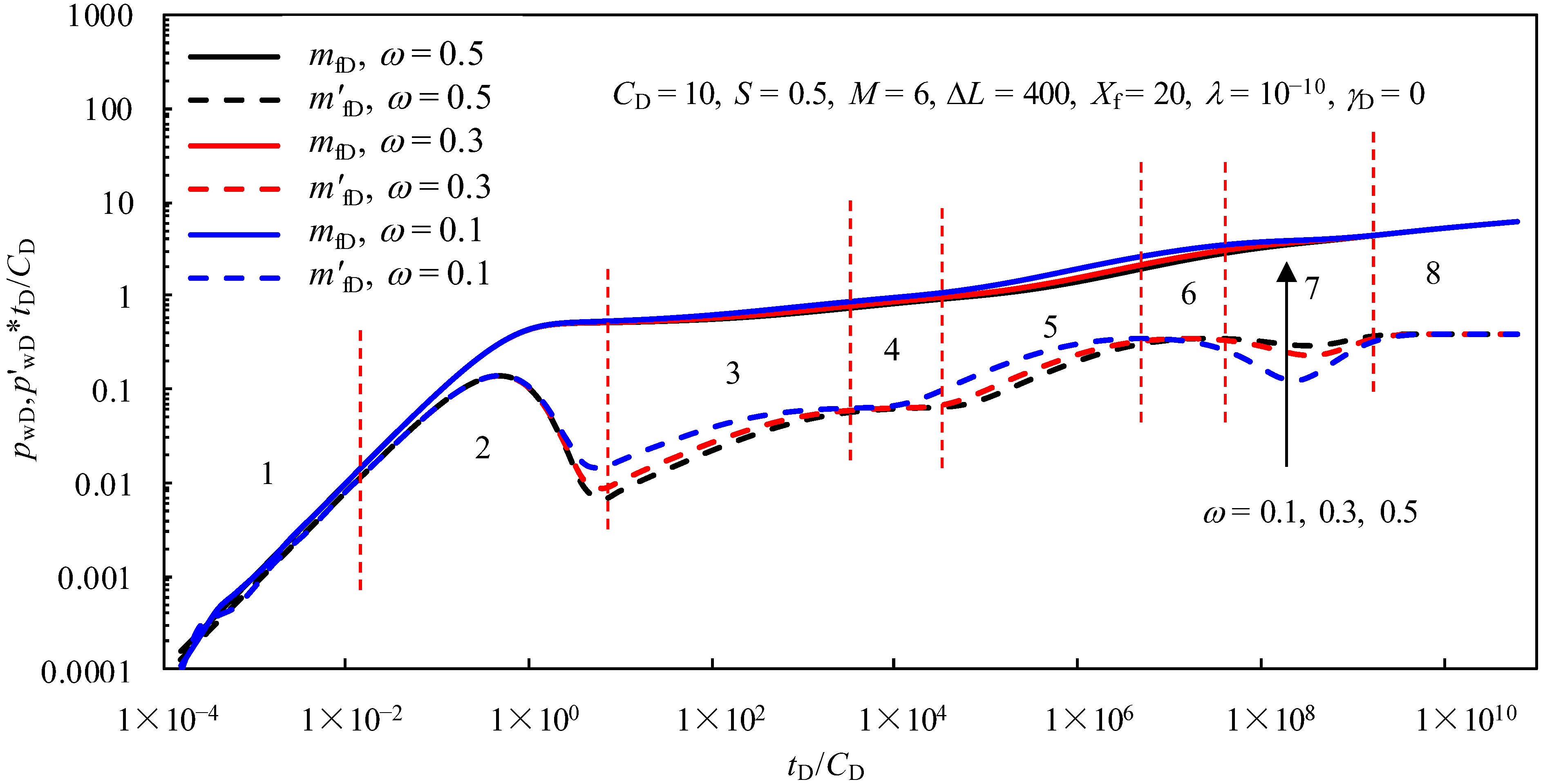
4.5. Effect of the Interporosity Flow Coefficient

Figure 7 shows the effect of the interporosity flow coefficient on the dimensionless pressure and pressure derivative curves. The interporosity flow coefficient mainly affects the time when the interporosity flow period occurs. The greater the value of λ, the faster shale oil in the matrix system interflows into the fracture system, so the dip shows up earlier in the pressure derivative curves.

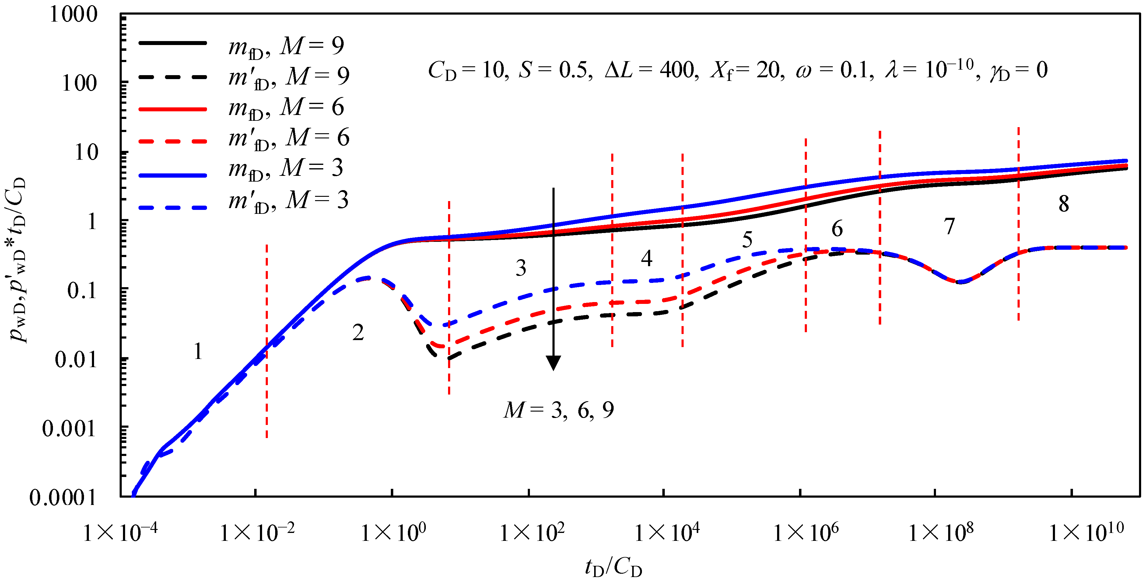
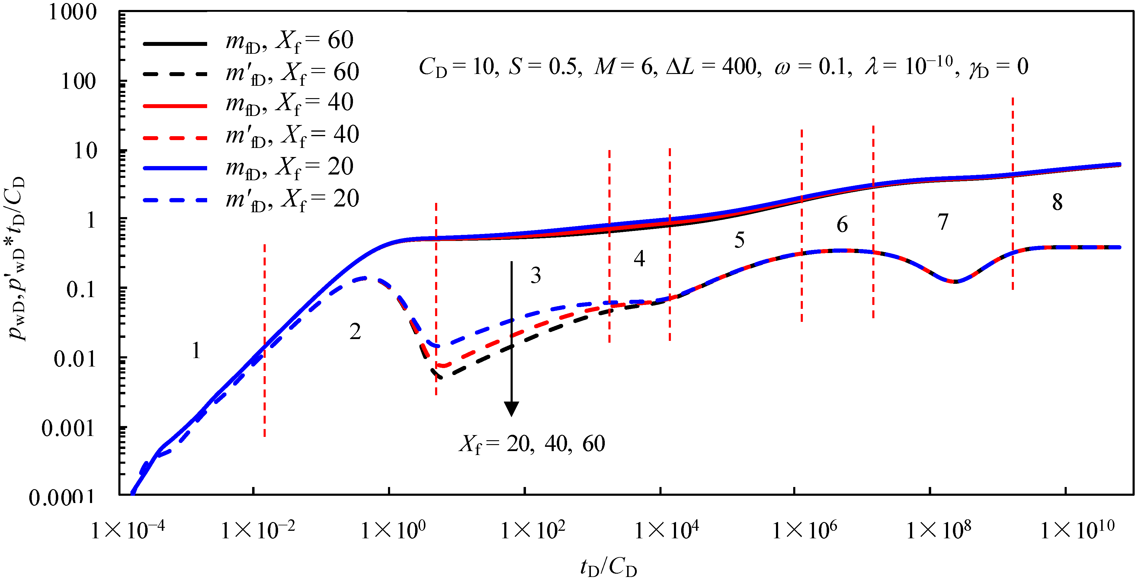
4.6. Effects of the Parameters of the Hydraulic Fractures

Figure 8 presents the effect of the number of transverse fractures on the dimensionless pressure and pressure derivative curves. It can be seen in the figure that the number of transverse fractures M mainly affects Periods 3, 4 and 5 of the typical curve. The greater the number of transverse fractures, the lower the pressure derivative curve is in the early and middle stages. Because increasing the number of transverse fractures significantly improves the flow capacity of the formation near the hydraulic fractures, a smaller pressure drop is needed for fluid flow.

Figure 9 shows the effect of the spacing of hydraulic fractures on the dimensionless pressure and pressure derivative curves. We can see in the figure that the spacing of the hydraulic fracture mainly affects the characteristics of the derivative curves in the early radial flow period. When the fracture’s half-length is constant, the smaller the fracture spacing is, and the interaction between the hydraulic fractures occurs earlier. Therefore, it is more difficult to form a pseudoradial flow of a single hydraulic fracture in the formation, and the earlier the second linear flow period appears.

Figure 10 presents the effect of different half-lengths of hydraulic fracture on the dimensionless pressure and pressure derivative curves. The longer a fracture’s half-length is, the larger the stimulated reservoir volume near the fracture is, and the longer the linear flow perpendicular to the hydraulic fracture plane lasts, so the pressure derivative curve will be lower. With an increase in the fracture’s half-length, the more difficult it is for a single fracture to form pseudoradial flow and the less obvious the characteristics of early radial flow are in the typical curve.

5. Conclusions

This study presents a multi-scale comprehensive dual porosity model for a fractured horizontal well in an inter-salt shale oil reservoir which considers the salt dissolution in the shale matrix and the stress-sensitive effect. The type curves under the effects of the related influencing parameters were analyzed. The following conclusions can be drawn.

(1)

The pressure response and corresponding pressure derivative curves of a MFHW in the inter-salt shale oil reservoir with consideration of the stress sensitivity of natural fractures were analyzed, and eight main flow periods could be observed in the type curves of transient pressure.

(2)

The influence of salt dissolution on the transient pressure curves of the fractured horizontal well in an inter-salt shale oil reservoir was negligible because the permeability decreased by only 5.06% when the average pressure dropped from 22.5 MPa to 7.5 MPa according to the experimental results of the effect of salt dissolution on the shale’s permeability.

(3)

The effect of the stress sensitivity of the fracture system on the pressure derivative curves became apparent in the radial flow period of natural fractures (Period 6). The pressure derivative curves gradually turned upward with an increase in the dimensionless permeability modulus. The stronger the stress sensitivity, the more serious the damage to the reservoir. It was therefore more difficult for the shale oil to flow, and greater drawdown pressure was required.

(4)

The effects of the storativity ratio, the interporosity flow coefficient and the parameters of the hydraulic fractures on the transient pressure curves were analyzed to better understand the transient flow behavior of the MFHW in an inter-salt shale oil reservoir.

References

1. Fan, X.; Su, J.Z.; Chang, X.; Huang, Z.W.; Zhou, T.; Guo, Y.T.; Wu, S.Q. Brittleness evaluation of the inter-salt shale oil reservoir in Jianghan Basin in China. Mar. Pet. Geol. 2019, 102, 109–115. [Google Scholar] [CrossRef]
2. Yang, L.; Lu, H.; Fan, X.; Huang, Z.; Zhou, T. Salt occurrence in matrix pores of intersalt shale oil reservoirs. Sci. Technol. Eng. 2020, 20, 1839–1845. [Google Scholar]
3. Li, Z.; Zhao, Y.; Wang, H.; Zhao, Q.; Lu, T.; Xu, Z. Effects of Injection Water Salinity on Physical Properties of Inter-Salt Shale Oil Reservoir. Spec. Oil Gas Reserv. 2020, 27, 131–137. [Google Scholar]
4. Zhang, Y.; Zhang, M.; Mei, H.; Zeng, F. Study on salt precipitation induced by formation brine flow and its effect on a high-salinity tight gas reservoir. J. Pet. Sci. Eng. 2019, 183, 106384. [Google Scholar] [CrossRef]
5. Kilmer, N.H.; Morrow, N.R.; Pitman, J.K. Pressure sensitivity of low permeability sandstones. J. Pet. Sci. Eng. 1987, 1, 65–81. [Google Scholar] [CrossRef]
6. Schutjens PM, T.M.; Hanssen, T.H.; Hettema MH, H.; Merour, J.; De Bree, P.; Coremans JW, A.; Helliesen, G. Compaction-Induced Porosity/Permeability Reduction in Sandstone Reservoirs: Data and Model for Elasticity-Dominated Deformation. SPE Reserv. Eval. Eng. 2004, 7, 202–216. [Google Scholar] [CrossRef]
7. Fatt, I.; Davis, T.H. The reduction in permeability with overburden pressure. Trans. AIME 1952, 4, 16. [Google Scholar] [CrossRef]
8. Mclatchie, A.; Hemstock, R.A.; Young, J.W. The effective compressiblity of reservoir rock and its effects on permeability. J. PetroI. Technol. 1952, 10, 49–51. [Google Scholar] [CrossRef]
9. Gray, D.H.; Fatt, I.; Bergarnini, G. The effect of stress on permeability of sandstone cores. Sot. Pet. Eng. J. 1963, 3, 95–100. [Google Scholar] [CrossRef]
10. Vairogs, J.; Hearn, C.L.; Dareing, D.W.; Rhoades, V.W. Effect of rock stress on gas production from low perrneability resevoirs. J. Pet. Technol. 1971, 23, 1161. [Google Scholar] [CrossRef]
11. Zhang, M.Y.; Ambastha, A.K. New insights in pressure-transient analysis for stress-sensitive reservoirs. Presented at the SPE Annual Technical Conference and Exhibition, New Orleans, LA, USA, 25–28 September 1994. [Google Scholar] [CrossRef]
12. Chin, L.Y.; Raghavan, R.; Thomas, L.K. Fully coupled geomechanics and fluid-flow analysis of wells with stress-dependent permeability. Soc. Petroleum Eng. 2000, 5, 32–45. [Google Scholar] [CrossRef]
13. Franquet, M.; Ibrahim, M.; Wattenbarger, R.A.; Maggard, J.B. Effect of pressure dependent permeability in tight gas reservoirs, transient radial flow. Presented at the Canadian International Petroleum Conference, Calgary, AB, Canada, 8–10 June 2004. [Google Scholar] [CrossRef]
14. Ali, T.A.; Sheng, J.J. Evaluation of the effect of stress-dependent permeability on production performance in shale gas reservoirs. Presented at the SPE Eastern Regional Meeting, Morgantown, WV, USA, 13–15 October 2015. [Google Scholar] [CrossRef]
15. Barenblatt, G.I.; Zheltov, Y.P. Fundamental equations of filtration of homogeneous liquids in fissured rocks. Sov. Phys. Dokl. 1960, 5, 522. [Google Scholar]
16. Warren, J.E.; Root, P.J. The behavior of naturally fractured reservoirs. Sot Pet. Eng. 1963, 228, 245–255. [Google Scholar] [CrossRef] [Green Version]
17. Rahman, M.K.; Rahman, M.M.; Joarder, A.H. Analytical Production Modeling for Hydraulically Fractured Gas Reservoirs. Pet. Sci. Technol. 2007, 25, 683–704. [Google Scholar] [CrossRef]
18. Rahman, M.M. Productivity Prediction for Fractured Wells in Tight Sand Gas Reservoirs Accounting for Non-Darcy Effects. Presented at the Russian Oil & Gas Technical Conference and Exhibition, Moscow, Russia, 28–30 October 2008. [Google Scholar] [CrossRef]
19. Xie, W.; Li, X.; Zhang, L.; Wang, J.; Cao, L.; Yuan, L. Two-phase pressure transient analysis for multi-stage fractured horizontal well in shale gas reservoirs. J. Nat. Gas Sci. Eng. 2014, 21, 691–699. [Google Scholar] [CrossRef]
20. Xu, Y.; Li, X.; Liu, Q.; Tan, X. Pressure performance of multi-stage fractured horizontal well considering stress sensitivity and dual permeability in fractured gas reservoirs. J. Pet. Sci. Eng. 2020, 201, 108154. [Google Scholar] [CrossRef]
21. Guo, J.; Wang, H.; Zhang, L. Transient pressure and production dynamics of multi-stage fractured horizontal wells in shale gas reservoirs with stimulated reservoir volume. J. Nat. Gas Sci. Eng. 2016, 35, 425–443. [Google Scholar] [CrossRef]
22. Xu, Y.; Li, X.; Liu, Q. Pressure performance of multi-stage fractured horizontal well with stimulated reservoir volume and irregular fractures distribution in shale gas reservoirs. J. Nat. Gas Sci. Eng. 2020, 77, 103209. [Google Scholar] [CrossRef]
23. Zongxiao, R.; Zhan, Q.; Huayi, J.; Erbiao, L.; Jiaming, Z.; Ze, Y.; Hongbin, Y. Transient pressure behaviour of multi-stage fractured horizontal well in stress-sensitive coal seam. Int. J. Oil Gas Coal Technol. 2019, 22, 163. [Google Scholar] [CrossRef]
24. Ren, J.; Guo, P.; Peng, S.; Ma, Z. Performance of multi-stage fractured horizontal wells with stimulated reservoir volume in tight gas reservoirs considering anomalous diffusion. Environ. Earth Sci. 2018, 77, 768. [Google Scholar] [CrossRef]
25. Zongxiao, R.; Xiaodong, W.; Guoqing, H.; Lingyan, L.; Xiaojun, W.; Guanghui, Z.; Hun, L.; Jiaming, Z.; Xianwei, Z. Transient pressure behavior of multi-stage fractured horizontal wells in stress-sensitive tight oil reservoirs. J. Pet. Sci. Eng. 2017, 157, 1197–1208. [Google Scholar] [CrossRef]
26. Li, X.P.; Cao, L.N.; Luo, C.; Zhang, B.; Zhang, J.Q.; Tan, X.H. Characteristics of transient production rate performance of horizontal well in fractured tight gas reservoirs with stress-sensitivity effect. J. Pet. Sci. Eng. 2017, 158, 92–106. [Google Scholar] [CrossRef]
27. Pedrosa, O.A. Pressure transient response in stress-sensitive formations. In Proceedings of the SPE California Regional Meeting, Oakland, CA, USA, 2–4 April 1986; pp. 203–210. [Google Scholar]
28. Kikani, J.; Pedrosa, O.A. Perturbation analysis of stress-sensitive reservoirs. SPE Form. Eval. 1991, 6, 379–396. [Google Scholar] [CrossRef]
29. Yeung, K.; Chakrabarty, C.; Zhang, X. An approximate analytical study of aquifers with pressure-sensitive formation permeability. Water Resour. Res. 1993, 29, 3495–3501. [Google Scholar] [CrossRef]
30. Van Everdingen, A.F.; Hurst, W. The application of the Laplace transformation to flow problems in reservoirs. Trans. AIME 1949, 186, 97–104. [Google Scholar] [CrossRef]
31. Stehfest, H. Algorithm 368: Numerical inversion of Laplace transforms. Commun. ACM 1970, 13, 47–49. [Google Scholar] [CrossRef]
32. Bumb, A.C.; McKee, C.R. Gas-well testing in the presence of desorption for coalbed methane and devonian shale. SPE Form. Eval. 1988, 3, 179–185. [Google Scholar] [CrossRef]
33. Zhan, H.; Zlotnik, V.A. Groundwater flow to horizontal and slanted wells in unconfined aquifers. Wat. Resour. Res. 2002, 38, 1108. [Google Scholar] [CrossRef] [Green Version]
34. Zhao, Y.; Zhang, L.; Zhao, J.; Luo, J.; Zhang, B. “Triple porosity” modeling of transient well test and rate decline analysis for multi-fractured horizontal well in shale gas reservoirs. J. Pet. Sci. Eng. 2013, 110, 253–261. [Google Scholar] [CrossRef]
35. Gao, Y.; Rahman, M.M.; Lu, J. Novel mathematical model for transient pressure analysis of multi-fractured horizontal well in naturally-fractured oil reservoir. ACS Omega 2021, 6, 15205–15221. [Google Scholar] [CrossRef]
Figure 1. Physical model of a MFHW in an inter-salt shale oil reservoir.
Processes 10 02085 g001
Figure 2. Physical model of a multi-stage fractured horizontal well.
Processes 10 02085 g002
Figure 3. Bilogarithmic type curve of the dimensionless pressure and the pressure derivatives of a MFHW in an inter-salt shale oil reservoir.
Processes 10 02085 g003
Figure 4. The effect of salt dissolution on the dimensionless pressure and pressure derivatives of a MFHW in an inter-salt shale oil reservoir.
Processes 10 02085 g004
Figure 5. The effect of stress sensitivity on the dimensionless pressure and pressure derivatives of a MFHW in an inter-salt shale oil reservoir.
Processes 10 02085 g005
Figure 6. The effect of the storativity ratio on the dimensionless pressure and pressure derivatives of a MFHW in an inter-salt shale oil reservoir.
Processes 10 02085 g006
Figure 7. The effect of the interporosity flow coefficient on the dimensionless pressure and pressure derivatives of a MFHW in an inter-salt shale oil reservoir.
Processes 10 02085 g007
Figure 8. The effect of the number of transverse fractures on the dimensionless pressure and pressure derivatives of a MFHW in an inter-salt shale oil reservoir.
Processes 10 02085 g008
Figure 9. The effect of the spacing of hydraulic fractures on the dimensionless pressure and pressure derivatives of a MFHW in an inter-salt shale oil reservoir.
Processes 10 02085 g009
Figure 10. The effect of the fracture’s half-length on the dimensionless pressure and pressure derivatives of a MFHW in an inter-salt shale oil reservoir.
Processes 10 02085 g010