


Temperature Prediction Model for a Regenerative Aluminum Smelting Furnace by a Just-in-Time Learning-Based Triple-Weighted Regularized Extreme Learning Machine


Abstract
:1. Introduction
2. Related Methods
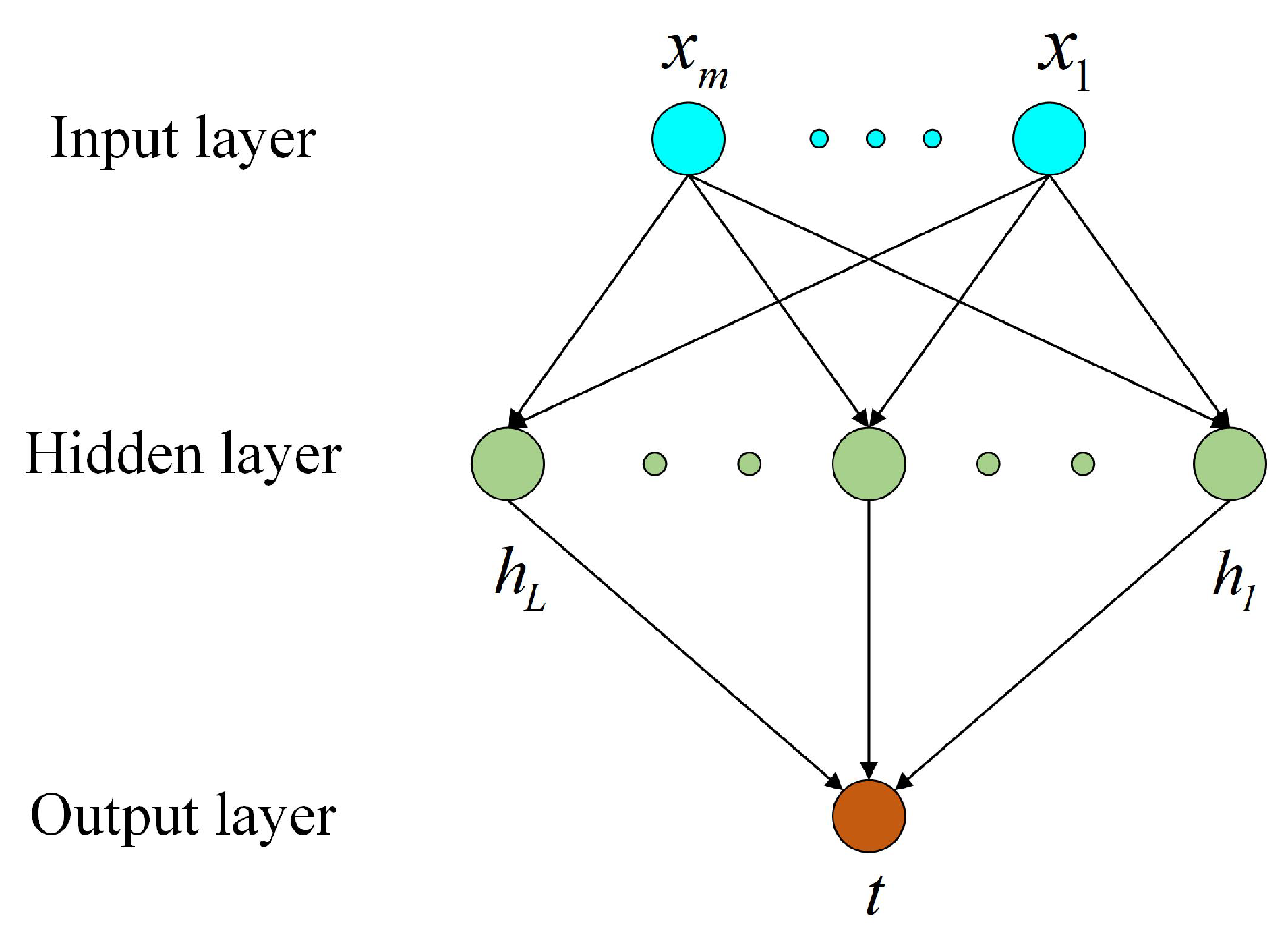
2.1. RELM
2.2. SWRELM
2.3. VWRELM
3. The Proposed JITL-TWRELM Model
3.1. Weighted Similarity Measurement Criterion
3.2. JITL-TWRELM
4. Industrial Case
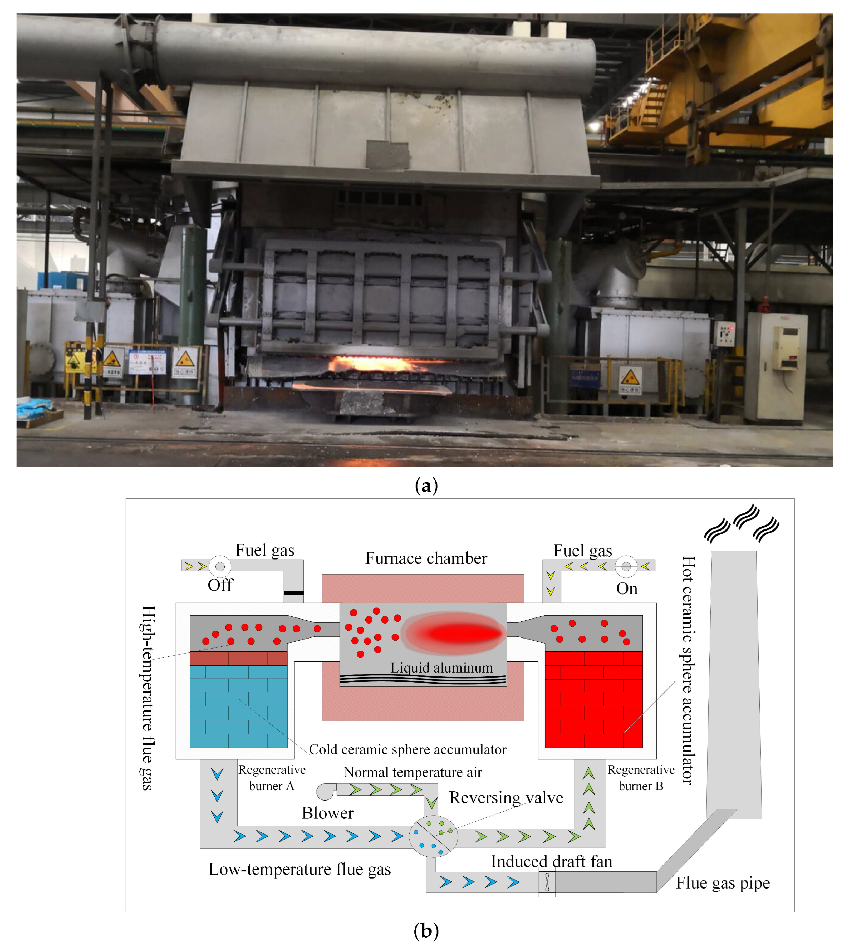
4.1. Process Description of the Regenerative Aluminum Smelting Furnace
4.2. Model Establishment
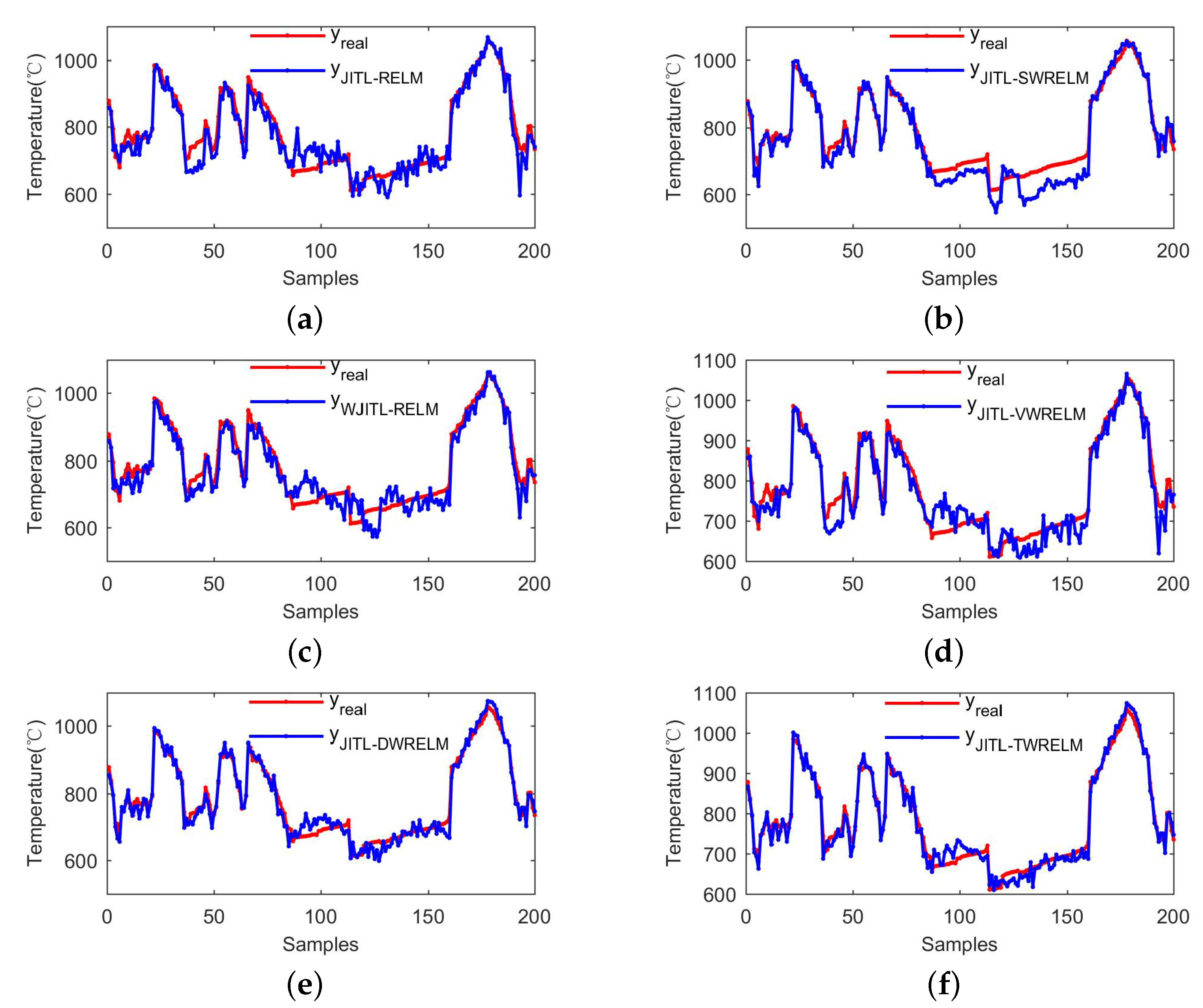
- Method 1: JITL-RELM (it applies the original JITL strategy and original RELM).
- Method 2: JITL-SWRELM (it applies the original JITL strategy and sample weights on RELM).
- Method 3: WJITL-RELM (it applies the WJITL strategy and original RELM).
- Method 4: JITL-VWRELM (it applies the original JITL strategy and local variable weights on RELM).
- Method 5: JITL-DWRELM (it applies the WJITL strategy and sample weights on RELM).
- Method 6: JITL-TWRELM (it applies the WJITL strategy, sample weights, and local variable weights on RELM).
4.3. Results and Discussion
5. Conclusions
Author Contributions
Funding
Data Availability Statement
Conflicts of Interest
References
- Froehlich, C.; Strommer, S.; Steinboeck, A.; Niederer, M.; Kugi, A. Modeling of the media supply of gas burners of an industrial furnace. IEEE Trans. Ind. Appl. 2016, 52, 2664–2672. [Google Scholar] [CrossRef]
- Strommer, S.; Niederer, M.; Steinboeck, A.; Kugi, A. A mathematical model of a direct-fired continuous strip annealing furnace. Int. J. Heat Mass Trans. 2014, 69, 375–389. [Google Scholar] [CrossRef]
- Qiu, L.; Feng, Y.H.; Chen, Z.G.; Li, Y.L.; Zhang, X.X. Numerical simulation and optimization of the melting process for the regenerative aluminum melting furnace. Appl. Therm. Eng. 2018, 145, 315–327. [Google Scholar] [CrossRef]
- Li, D.Y.; Song, Z.H. A novel incremental gaussian mixture regression and its application for time-varying multimodal process quality prediction. In Proceedings of the 2020 IEEE 9th Data Driven Control and Learning Systems Conference, Liuzhou, China, 19–21 June 2020. [Google Scholar]
- Bao, L.; Yuan, X.F.; Ge, Z.Q. Co-training partial least squares model for semi-supervised soft sensor development. Chemometr. Intell. Lab. 2015, 147, 75–85. [Google Scholar] [CrossRef]
- Wang, G.; Luo, H.; Peng, K.X. Quality-related fault detection using linear and nonlinear principal component regression. J. Franklin. Inst. 2016, 353, 2159–2177. [Google Scholar] [CrossRef]
- Liu, H.B.; Yang, C.; Huang, M.Z.; ChangKyoo, Y. Soft sensor modeling of industrial process data using kernel latent variables-based relevance vector machine. Appl. Soft. Comput. 2020, 90, 106149. [Google Scholar] [CrossRef]
- Shi, X.; Huang, G.L.; Hao, X.C.; Yang, Y.; Li, Z. A Synchronous Prediction Model Based on Multi-Channel CNN with Moving Window for Coal and Electricity Consumption in Cement Calcination Process. Sensors 2021, 21, 4284. [Google Scholar] [CrossRef]
- Zhe, L.; Yi-Shan, L.; Chen, J.H.; Qian, Y.W. Developing variable moving window PLS models: Using case of NOx emission prediction of coal-fired power plants. Fuel 2021, 296, 120441–120456. [Google Scholar]
- Mai, T.; Yu, X.L.; Gao, S.; Frejinger, E. Routing policy choice prediction in a stochastic network: Recursive model and solution algorithm. Transport. Res. B-Methodol. 2021, 151, 42–58. [Google Scholar] [CrossRef]
- Doshi, P.; Gmytrasiewicz, P.; Durfee, E. Recursively modeling other agents for decision making: A research perspective. Artif. Intell. 2020, 279, 103202–103220. [Google Scholar] [CrossRef]
- Qiu, K.P.; Wang, J.L.; Zhou, X.J.; Guo, Y.Q.; Wang, R.T. Soft sensor framework based on semisupervised just-in-time relevance vector regression for multiphase batch processes with unlabeled data. Ind. Eng. Chem. Res. 2020, 59, 19633–19642. [Google Scholar] [CrossRef]
- Wu, Y.J.; Liu, D.J.; Yuan, X.F.; Wang, Y.L. A just-in-time fine-tuning framework for deep learning of SAE in adaptive data-driven modeling of time-varying industrial processes. IEEE. Sens. J. 2020, 21, 3497–3505. [Google Scholar] [CrossRef]
- Chen, N.; Luo, L.H.; Gui, W.H.; Guo, Y.Q. Integrated modeling for roller kiln temperature prediction. In Proceedings of the 2017 Chinese Automation Congress, Shandong, China, 20–22 October 2017. [Google Scholar]
- Dai, J.Y.; Chen, N.; Yuan, X.F.; Gui, W.H.; Luo, L.H. Temperature prediction for roller kiln based on hybrid first-principle model and data-driven MW-DLWKPCR model. ISA Trans. 2020, 98, 403–417. [Google Scholar] [CrossRef]
- Yao, L.; Ge, Z.Q. Locally weighted prediction methods for latent factor analysis with supervised and semisupervised process data. IEEE Trans. Autom. Sci. Eng. 2016, 14, 126–138. [Google Scholar] [CrossRef]
- Chen, J.M.; Yang, C.H.; Zhou, C.; Li, Y.G.; Zhu, H.Q.; Gui, W.H. Multivariate regression model for industrial process measurement based on double locally weighted partial least squares. IEEE. Trans. Instrum. Meas. 2019, 69, 3962–3971. [Google Scholar] [CrossRef]
- Yuan, X.F.; Huang, B.; Ge, Z.Q.; Song, Z.H. Double locally weighted principal component regression for soft sensor with sample selection under supervised latent structure. Chemometr. Intell. Lab. 2018, 153, 116–125. [Google Scholar] [CrossRef]
- Lin, W.L.; Hang, H.F.; Zhuang, Y.P.; Zhang, S.L. Variable selection in partial least squares with the weighted variable contribution to the first singular value of the covariance matrix. Chemometr. Intell. Lab. 2018, 183, 113–121. [Google Scholar] [CrossRef]
- Yuan, X.F.; Li, L.; Shardt, Y.; Wang, Y.L.; Yang, C.H. Deep learning with spatiotemporal attention-based LSTM for industrial soft sensor model development. IEEE Trans. Ind. Electron. 2020, 65, 4404–4414. [Google Scholar] [CrossRef]
- Yuan, X.F.; Li, L.; Wang, Y.L. Nonlinear dynamic soft sensor modeling with supervised long short-term memory network. IEEE Trans. Ind. Inform. 2019, 16, 3168–3176. [Google Scholar] [CrossRef]
- He, Z.S.; Chen, Y.H.; Xu, J. A Combined Model Based on the Social Cognitive Optimization Algorithm for Wind Speed Forecasting. Processes 2022, 10, 689. [Google Scholar] [CrossRef]
- Wang, X.L.; Zhang, H.; Wang, Y.L.; Yang, S.M. ELM-Based AFL–SLFN Modeling and Multiscale Model-Modification Strategy for Online Prediction. Processes 2019, 7, 893. [Google Scholar] [CrossRef] [Green Version]
- Li, G.Q.; Chen, B.; Qi, X.B.; Zhang, L. Circular convolution parallel extreme learning machine for modeling boiler efficiency for a 300 MW CFBB. Soft. Comput. 2019, 23, 6567–6577. [Google Scholar] [CrossRef]
- Hu, P.H.; Tang, C.X.; Zhao, L.C.; Liu, S.L.; Dang, X.M. Research on measurement method of spherical joint rotation angle based on ELM artificial neural network and eddy current sensor. IEEE Sens. J. 2021, 21, 12269–12275. [Google Scholar] [CrossRef]
- Su, X.L.; Zhang, S.; Yin, Y.X.; Xiao, W.D. Prediction model of hot metal temperature for blast furnace based on improved multi-layer extreme learning machine. Int. J. Mach. Learn. Cybern. 2019, 10, 2739–2752. [Google Scholar] [CrossRef]
- Huang, Q.B.; Lei, S.N.; Jiang, C.L.; Xu, C.H. Furnace Temperature Prediction of Aluminum Smelting Furnace Based on KPCA-ELM. In Proceedings of the 2018 Chinese Automation Congress, Xi’an, China, 30 November–2 December 2018. [Google Scholar]
- Liu, Q.; Wei, J.; Lei, S.; Huang, Q.B.; Zhang, M.Q.; Zhou, X.B. Temperature prediction modeling and control parameter optimization based on data driven. In Proceedings of the 2020 IEEE Fifth International Conference on Data Science in Cyberspace, Hong Kong, China, 24–27 June 2020. [Google Scholar]
- Li, Z.X.; Hao, K.R.; Chen, L.; Ding, Y.S.; Huang, B. Pet viscosity prediction using jit-based extreme learning machine. In Proceedings of the 2018 IFAC Conference, Changchun, China, 20–22 September 2018. [Google Scholar]
- Wang, Y.; Li, Y.G.; Wu, B.Y. Improved regularized extreme learning machine short-term wind speed prediction based on gray correlation analysis. Wind. Eng. 2021, 45, 667–679. [Google Scholar]
- Pan, Z.Z.; Meng, Z.; Chen, Z.J.; Gao, W.Q.; Shi, Y. A two-stage method based on extreme learning machine for predicting the remaining useful life of rolling-element bearings. Mech. Syst. Signal Process. 2020, 144, 106899–106916. [Google Scholar] [CrossRef]
- Zong, W.W.; Huang, G.B.; Chen, Y.Q. Weighted extreme learning machine for imbalance learning. Neurocomputing 2013, 101, 229–242. [Google Scholar] [CrossRef]
- Chen, N.; Dai, J.Y.; Yuan, X.F.; Gui, W.H.; Ren, W.T.; Koivo, H. Temperature prediction model for roller kiln by ALD-based double locally weighted kernel principal component regression. IEEE Trans. Instrum. Meas. 2018, 67, 2001–2010. [Google Scholar] [CrossRef]


| Symbols | Definition |
|---|---|
| the nth historical input and output variable vectors | |
| the output weight of the ith hidden layer unit | |
| , , , | the output weight vectors in RELM, SWRELM, VWRELM, JITL-TWRELM |
| T | the output vector of RELM |
| , | the input weight and bias connecting input layer and ith hidden layer unit |
| , | the output corresponding to , the output of the query sample in JITL-TWRELM |
| N | the number of training samples |
| C | the regularization coefficient |
| the training error vector | |
| H,, | the hidden layer output matrices in RELM, VWRELM, JITL-TWRELM |
| the sample weight of the nth sample, the sample weighted matrix, the sample weighted matrix in JITL-TWRELM | |
| the Lagrange multiplier vector | |
| the Pearson correlation coefficient | |
| , | the expectation of the single input variable and output variable |
| the contribution of each variable | |
| V | the variable contribution matrix |
| the variable weighted input sample, the variable weighted local modeling sample | |
| the original Euclidean distance and weighted Euclidean distance, the weighted Euclidean distance in JITL-TWRELM | |
| the query sample, the variable weighted query sample in JITL-TWRELM | |
| the correlation coefficient matrix, the local correlation coefficient matrix, the global correlation coefficient matrix | |
| the adjusted parameter | |
| the local modeling sample matrix, the variable weighted local modeling sample matrix in JITL-TWRELM |
| Method | Shortcomings |
|---|---|
| RELM | Neither sample similarities nor variable correlations are considered, and the model cannot be updated in real-time. |
| SWRELM | Only the sample similarities are considered, no variable correlations are considered, and the model cannot be updated in real-time. |
| VWRELM | Only the variable correlations are considered, no sample similarities are considered, and the model cannot be updated in real-time. |
| Input | Variable |
|---|---|
| 1 | Material temperature |
| 2 | Furnace pressure |
| 3 | 12 # combustion airflow |
| 4 | 12 # combustion air pressure difference |
| 5 | 34 # combustion airflow |
| 6 | 34 # combustion air temperature |
| 7 | 34 # combustion air pressure difference |
| 8 | 34 # gas air-fuel ratio |
| 9 | B1 # exhaust gas temperature |
| 10 | B2 # exhaust gas temperature |
| 11 | B3 # exhaust gas temperature |
| 12 | B4 # combustion air temperature |
| Sensor Type | Measurement Range | Measurement Error |
|---|---|---|
| Pressure meter | 0–15,000 Pa | 1% |
| Flow meter | 0–15 m3/h | 1.5% |
| Thermocouple | 0–1300 °C | 1% |
| C | ||||
|---|---|---|---|---|
| 140 | 15.0884 | 18.6443 | 0.020354 | 0.98666 |
| 150 | 14.7273 | 17.9456 | 0.019897 | 0.98764 |
| 160 | 15.3797 | 19.5019 | 0.020879 | 0.98541 |
| 170 | 15.5217 | 20.4519 | 0.021023 | 0.98395 |
| 180 | 15.8944 | 20.1194 | 0.021629 | 0.98447 |
| 190 | 16.0543 | 19.8318 | 0.021839 | 0.98491 |
| 200 | 17.1959 | 22.2015 | 0.023265 | 0.98109 |
| Dataset | Method | ||||
|---|---|---|---|---|---|
| D1 | JITL-RELM | 43.0278 | 52.4279 | 0.062519 | 0.89453 |
| JITL-SWRELM | 38.1265 | 47.9605 | 0.052589 | 0.91174 | |
| WJITL-RELM | 32.7444 | 42.7606 | 0.044443 | 0.92984 | |
| JITL-VWRELM | 38.0149 | 46.1055 | 0.054197 | 0.91843 | |
| JITL-DWRELM | 20.7980 | 24.5347 | 0.029768 | 0.97690 | |
| JITL-TWRELM | 14.7273 | 17.9456 | 0.019897 | 0.98764 | |
| D2 | JITL-RELM | 26.7981 | 36.1509 | 0.035878 | 0.90223 |
| JITL-SWRELM | 26.3624 | 33.526 | 0.03657 | 0.91174 | |
| WJITL-RELM | 27.4121 | 34.5595 | 0.044443 | 0.91065 | |
| JITL-VWRELM | 24.3605 | 31.4511 | 0.032461 | 0.92600 | |
| JITL-DWRELM | 16.2472 | 22.2734 | 0.021632 | 0.96289 | |
| JITL-TWRELM | 14.8733 | 18.5463 | 0.019646 | 0.97427 |
Publisher’s Note: MDPI stays neutral with regard to jurisdictional claims in published maps and institutional affiliations. |
© 2022 by the authors. Licensee MDPI, Basel, Switzerland. This article is an open access article distributed under the terms and conditions of the Creative Commons Attribution (CC BY) license (https://creativecommons.org/licenses/by/4.0/).
Share and Cite
Chen, X.; Dai, J.; Luo, Y. Temperature Prediction Model for a Regenerative Aluminum Smelting Furnace by a Just-in-Time Learning-Based Triple-Weighted Regularized Extreme Learning Machine. Processes 2022, 10, 1972. https://doi.org/10.3390/pr10101972
Chen X, Dai J, Luo Y. Temperature Prediction Model for a Regenerative Aluminum Smelting Furnace by a Just-in-Time Learning-Based Triple-Weighted Regularized Extreme Learning Machine. Processes. 2022; 10(10):1972. https://doi.org/10.3390/pr10101972
Chicago/Turabian StyleChen, Xingyu, Jiayang Dai, and Yasong Luo. 2022. "Temperature Prediction Model for a Regenerative Aluminum Smelting Furnace by a Just-in-Time Learning-Based Triple-Weighted Regularized Extreme Learning Machine" Processes 10, no. 10: 1972. https://doi.org/10.3390/pr10101972
APA StyleChen, X., Dai, J., & Luo, Y. (2022). Temperature Prediction Model for a Regenerative Aluminum Smelting Furnace by a Just-in-Time Learning-Based Triple-Weighted Regularized Extreme Learning Machine. Processes, 10(10), 1972. https://doi.org/10.3390/pr10101972