Virtual Voltage Vector-Based Model Predictive Current Control for Five-Phase Induction Motor

Abstract

The high-performance control technology of multi-phase motors is a key technology for the application of multi-phase motors in many fields, such as electric transportation. The model predictive current control (MPCC) strategy has been extended to multi-phase systems due to its high dynamic performance. Model-predictive current control faces the problem that it cannot effectively regulate harmonic plane currents, and thus cannot obtain high-quality current waveforms because only one switching state is applied in a sampling period. To solve this problem, this paper uses the virtual vector-based MPCC to select the optimal virtual vector and apply it under the premise that the average value of the harmonic plane voltage in a single switching cycle is zero. Taking a five-phase induction motor as an example, the steady-state and dynamic performance of the proposed virtual vector MPCC and the traditional model predictive current control were simulated, respectively. Simulation results demonstrated the effectiveness of the proposed method in improving waveform quality while maintaining excellent dynamic performance.

1. Introduction

Due to the massive consumption of fossil energy and the increasingly serious air pollution problems caused by the exhaust emissions of fuel vehicles, new energy systems focusing on green and low-carbon development have achieved great progress. Vehicles utilizing new forms of energy with low pollution emissions are an important application of new energy systems in transportation; as an example, pure electric vehicles and hybrid vehicles are gradually gaining favor in the market [1,2]. The motor is a key component of new energy vehicles; excellent motor control technology directly affects the operation and safety performance of electric vehicles, so a high-performance motor and its control technology are very important for the development of electric vehicles [3,4]. Usually, variable-speed AC drives are powered by power electronic converters, but with the development of power electronic technology, the phase number of the motor is no longer restricted by the traditional three-phase power supply. The multi-phase motor drive system has received a lot of attention and research in the fields of ship power propulsion, aerospace and so on [5,6]. Compared with the traditional three-phase system, the multi-phase motor drive system has the following advantages: (1) high reliability and strong fault tolerance [7,8]; (2) low voltage and high power drive can be realized by the reduction of per-phase current [9]; and (3) low torque ripple reduces vibration and noise [10]. Among the various multi-phase drive system solutions, the five-phase system is a typical representative, which has the typical advantages of the multi-phase system and a relatively simple structure [11].

Model predictive control (MPC) first appeared in the 1960s and was applied in the chemical industry. With the rapid development of microprocessors, MPC schemes have been extended to the fields of power electronics and have been widely researched and applied [12,13]. As one of the most commonly used schemes, finite-control-set model predictive control (FCS-MPC) has the advantages of simple structure, fast dynamic response, simple concept, and easy handling of nonlinear multivariable constraints [14,15]. FCS-MPC uses the discrete characteristics of the inverter output to enumerate all the alternative voltage vectors and select the optimal voltage vector as the output by minimizing the cost function, eliminating the need for pulse width modulation [16,17]. For motor systems, FCS-MPC can be further divided into two categories, namely model-predictive current control (MPCC) and model-predictive torque control (MPTC). Since the cost function in the model-predicted torque includes two variables with different physical units, torque and flux linkage, it is difficult to select the weight coefficients [18]. Therefore, the MPCC scheme is more widely used.

Due to its high dynamic performance and flexibility to handle constraints, MPCC is replacing the most commonly used field-oriented control (FOC) in the field of motor control [19]. MPCC has been successfully extended from the three-phase motor drive system to the multiphase motor drive system, which proves the feasibility of model predictive current control in the multiphase system [20,21]. However, in the MPCC scheme of multiphase motors, it is often faced with the problem that too many alternative vectors lead to the complexity of the algorithm and an increase of the calculation amount. At the same time, due to the use of a single inverter-switching state, generating voltage in the harmonic plane of the multiphase motor is inevitable, so as to bring harmonic current, resulting in excess harmonic loss and affecting the performance of the system [22,23].

In order to solve the problem of the large computational load of model predictive control in multiphase systems, a simplified algorithm using adjacent voltage vectors was proposed in the literature [24], which reduced the number of alternative voltage vectors and was applied in multilevel cascade inverters. The literature [25] limited the number of switches in adjacent sampling periods in advance, so as to exclude some voltage vectors with a large number of switches and narrow the range of voltage vector candidates. In order to reduce the harmonic current of the multi-phase motor, the traditional MPC uses a cost function including two plane current tracking errors, but this method introduces a weighting factor, and the selection of the weighting factor is very troublesome and the harmonic current suppression effect is relatively general [15,22].

In order to eliminate the harmonic current of the multiphase motor from the source, this paper uses virtual voltage vectors (VVs) to solve this problem. The basic voltage vector is synthesized according to the fixed ratio of VVs, and the VVs are used as the set of selected vectors to carry out the model predictive current control of five-phase induction motor. In the literature [26], large vectors and medium vectors were used to synthesize virtual vectors and construct switching tables, and voltage vectors were selected for direct torque control according to torque, flux error and speed range. The literature [27] redefined a new virtual vector to realize fault-tolerant operation of the five-phase induction motor on the premise of open-circuit induction motor. The literature also [28,29] introduced the concept of virtual vectors into the model predictive current control of the six-phase induction motor, and proved that the use of virtual vectors can effectively reduce the loss and improve the quality of current waveform.

The remaining chapters are organized as follows. In the second part, the model of the five-phase induction motor and the two-level five-phase voltage source inverter is introduced, and the distribution characteristics of the basic voltage vector are given. The third part introduces the traditional model predictive current control scheme. The fourth part explains the process of virtual vector synthesis and implementation, and introduces the virtual vector MPC scheme proposed in this paper in detail. In the fifth part, the simulation results and analysis are presented. Finally, the sixth part gives the conclusion.

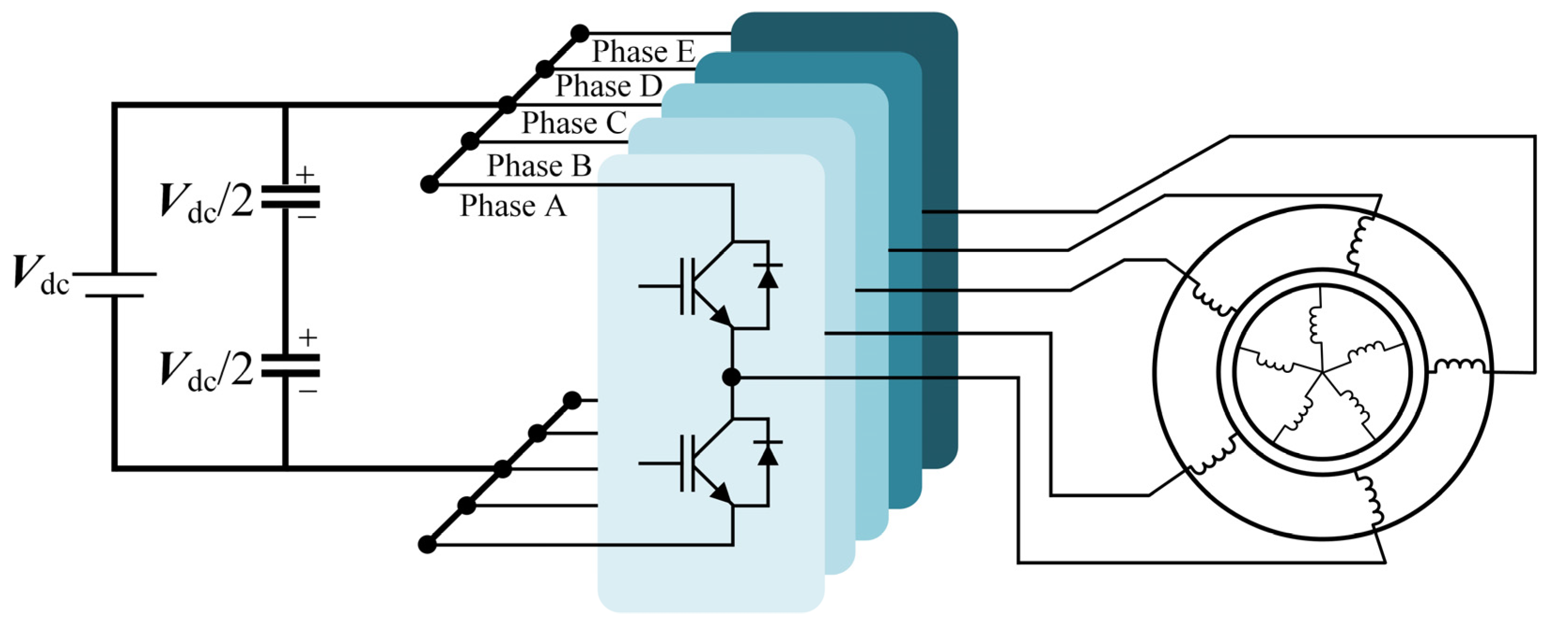
2. Five-Phase Induction Motor Drive

2.1. Five-Phase Induction Motor Model

Before using the model predictive current control strategy for the five-phase induction motor, it is necessary to establish the mathematical model of the five-phase inverter and the five-phase induction motor. The topology of the five-phase voltage source inverter and the five-phase induction motor connection system is shown in Figure 1. The motor windings are star-connected and the DC side voltage V_dc is considered constant.

Applying the decoupling transformation matrix of the five-phase system defined in (1), variables in the stationary coordinates of five-phase can be transformed into three normal subspaces in (2). They are the α-β subspace (fundamental subspace), the x-y subspace (third harmonic subspace), and the o1-o2 subspace (zero-sequence harmonic subspace), respectively:

$$T_{}=\sqrt{\frac{2}{5}}\left[\begin{array}{ccccc}1& \cos \alpha & \cos 2\alpha & \cos 3\alpha & \cos 4\alpha \\ 0& \sin \alpha & \sin 2\alpha & \sin 3\alpha & \sin 4\alpha \\ 1& \cos 3\alpha & \cos 6\alpha & \cos 9\alpha & \cos 12\alpha \\ 0& \sin 3\alpha & \sin 6\alpha & \sin 9\alpha & \sin 12\alpha \\ 1& 1& 1& 1& 1\end{array}\right]$$

(1)

$${\left[\begin{array}{ccccc}{x}_{\alpha }& x_{\beta }& x_x& x_y& x_o\end{array}\right]}^T=\left[T\right]\cdot {\left[\begin{array}{ccccc}{x}_1& x_2& x_3& x_4& x_5\end{array}\right]}^T$$

(2)

where α = 2π/5.

Therefore, the control of the five-phase motor can be realized through the control of these two two-dimensional spaces. The five-phase system includes four degrees of freedom and zero-sequence components. For a five-phase induction motor, the α-β subspace corresponds to the first and second rows of the decoupling matrix, x-y subspace corresponds to the third and fourth rows of the decoupling matrix, and the o1-o2 subspace corresponds to the last row of the decoupling matrix, respectively. These subspaces have the following characteristics:

(1) The three subspaces are orthogonal subspaces to each other.

(2) The α-β subspace generates rotating magnetomotive force, and the fundamental wave and (10n ± 1) harmonics in the magnetic flux of the motor winding are projected into this space, which is the electromechanical energy conversion subspace.

(3) The motor variable in the x-y subspace is the (10n ± 3) harmonic in the motor winding flux. This harmonic component does not generate rotating magnetic motive force and does not participate in electromechanical energy conversion, which will generate harmonic current and cause harmonic loss.

(4) The 5k (k = 1, 3, 5…) harmonics in the motor variables are projected into the zero-sequence harmonic subspace, which is usually negligible for a five-phase induction motor.

After decoupling transformation, the stator voltage equation of the five-phase induction motor is:

$$\begin{array}{l}{v}_{s\alpha }=(R_s+L_s\frac{d}{dt})i_{s\alpha }+L_m\frac{d{i}_{r\alpha }}{dt}\\ v_{s\beta }=(R_s+L_s\frac{d}{dt})i_{s\beta }+L_m\frac{d{i}_{r\beta }}{dt}\\ v_{sx}=(R_s+L_{ls}\frac{d}{dt})i_{sx}\\ v_{sy}=(R_s+L_{ls}\frac{d}{dt})i_{sy}\end{array}$$

(3)

The rotor voltage equation is:

$$\begin{array}{l}0=(R_r+L_r\frac{d}{dt})i_{r\alpha }+L_m\frac{d{i}_{s\alpha }}{dt}+{\omega }_r{L}_r{i}_{r\beta }+{\omega }_r{L}_m{i}_{s\beta }\\ 0=(R_r+L_r\frac{d}{dt})i_{r\beta }+L_m\frac{d{i}_{s\beta }}{dt}-{\omega }_r{L}_r{i}_{r\alpha }-{\omega }_r{L}_m{i}_{s\alpha }\end{array}$$

(4)

The torque equation is:

$$T_e=n_p{L}_m(i_{s\beta }{i}_{r\alpha }-i_{s\alpha }{i}_{r\beta })$$

(5)

where L_m is the equivalent mutual inductance between stator and rotor windings, and L_s and L_r are the equivalent self-inductance of the stator winding and stator winding, respectively. L_ls is the stator leakage inductance. n_p is the number of pole pairs. ω_r is the rotor electrical speed. R_s, R_r are the stator resistor and the rotor resistor. The subscripts “s” and “r” represent the stator-side and rotor-side variables, respectively.

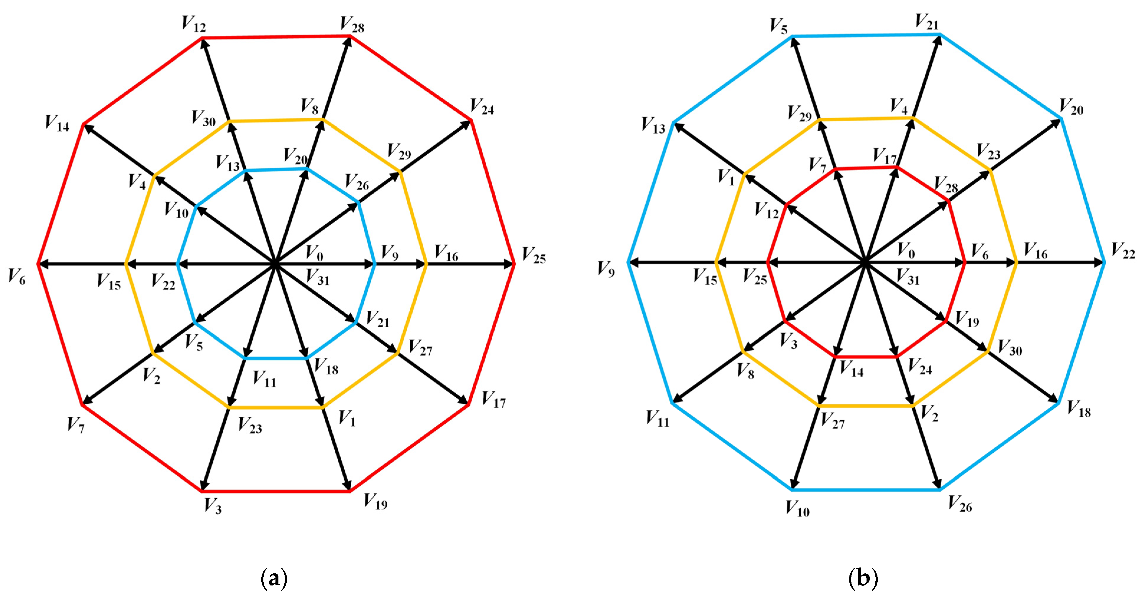
2.2. Voltage Vectors Distribution

The switch function can be defined as S_x, x∈{A,B,C,D,E}, where x = A,B,C,D,E represents the switching state of the inverter bridge arm, S_x = 1 represents that the upper arm of the bridge opens and the lower arm closes, while S_x = 0 represents that the lower arm opens and the upper arm closes. A total of 2⁵ = 32 switching states can be generated by the inverter phase number. Therefore, the stator phase voltage represented by switching state (S_x) and DC bus voltage (V_dc) is:

$$\left[\begin{array}{l}{U}_{\mathrm{ao}}\\ U_{\mathrm{bo}}\\ U_{\mathrm{co}}\\ U_{\mathrm{do}}\\ U_{\mathrm{eo}}\end{array}\right]=\frac{1}{5}{V}_{dc}\left[\begin{array}{ccccc}4& -1& -1& -1& -1\\ -1& 4& -1& -1& -1\\ -1& -1& 4& -1& -1\\ -1& -1& -1& 4& -1\\ -1& -1& -1& -1& 4\end{array}\right]\cdot \left[\begin{array}{c}{S}_A\\ S_B\\ S_C\\ S_D\\ S_E\end{array}\right]$$

(6)

By the decoupling transformation matrix (1), the stator phase voltage is mapped to two orthogonal subspaces and an additional zero-order subspace, and the voltage vector can be written as a switching state in two separate spaces:

$$\begin{array}{l}{V}_{\alpha -\beta }=V_{\alpha }+j{V}_{\beta }=\frac{2}{5}{V}_{dc}\left(S_a+a{S}_b+a^2{S}_c+a^3{S}_d+a^4{S}_e\right)\\ V_{x-y}=V_x+j{V}_y=\frac{2}{5}{V}_{dc}\left(S_a+a{S}_c+a^2{S}_e+a^3{S}_b+a^4{S}_d\right)\end{array}$$

(7)

where $a$ = exp(jπ2/5).

The distribution of 32 voltage vectors generated by the five-phase voltage source inverters in these two subspaces is shown in Figure 2.

These 32 voltage vectors consist of 2 zero vectors and 30 non-zero vectors, which can be grouped into three groups based on the magnitude of the voltage vector in the fundamental wave space: large vectors, medium vectors and small vectors. The specific groupings are shown in

Table 1. Space vector and vorresponding switching states.

Group	Switching States
Large	V25 (11001) V24(11000) V28 (11100)V12 (01100) V14 (01110) V6 (00110) V7 (00111) V3 (00011) V19 (10011) V17 (10001)
Medium	V16 (10000) V29 (11101) V8 (01000) V30 (11110) V4 (00100) V15 (01111) V2 (00010) V23 (10111) V1 (00001) V27 (11011)
Small	V9 (01001) V26 (11010) V20 (10100) V13 (01101) V10 (01010) V22 (10110) V5 (00101) V11 (01011) V18 (10010) V21 (10101)

. The amplitudes of each group of voltage vectors in the fundamental wave space are: 0.6472 V_dc, 0.4 V_dc, 0.2472 V_dc. Therefore, the voltage vector in α-β subspace can be divided into three decagons. From the outside to the inside, the ratio of the radius amplitudes of two adjacent decagons is 1.618.

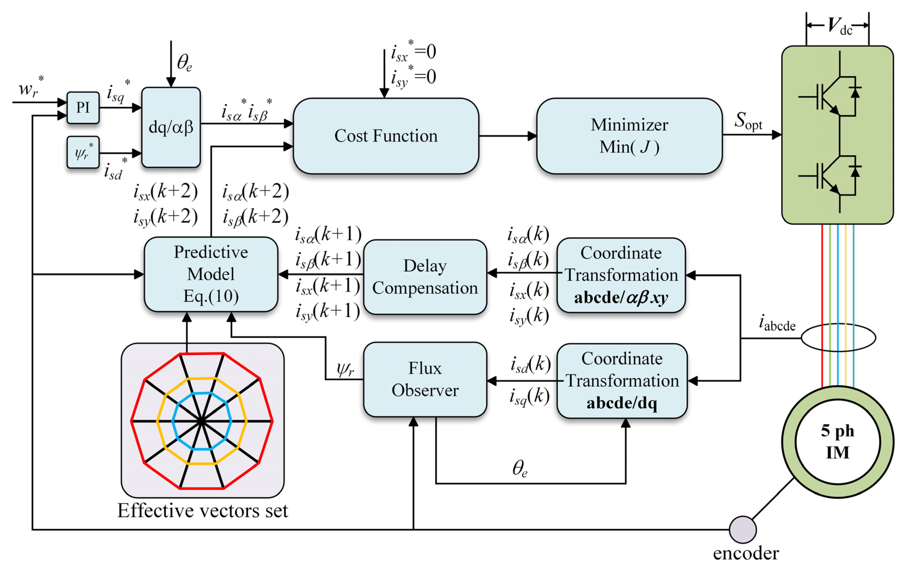
3. Traditional FCS-MPCC Scheme

3.1. Prediction Model of Induction Motor

In general, MPCC controls the stator current in the d-q coordinate system [22,30,31], but considering that there are 32 alternative voltage vectors for the two-level five-phase inverter, if the control is still carried out in the d-q coordinate system, there are 32 candidate voltage vectors needed to carry out the rotation transformation into the d-q coordinate system. In order to reduce the number of rotation transformations, the control is carried out in the α-β two-phase stationary coordinate system [14,17]. It is necessary to transform the generated given current from the d-q coordinate system to the α-β two-phase stationary coordinate system, and the number of rotation transformations is reduced to only once. The structure of traditional FCS-MPCC scheme is shown in the Figure 3.

In the α-β two-phase coordinate system, the stator current and rotor flux linkage of the motor are selected as state variables:

$$X_{\alpha \beta xy}={\left[\begin{array}{cccccc}{i}_{s\alpha }& i_{s\beta }& i_{sx}& i_{sy}& {\psi }_{r\alpha }& {\psi }_{r\beta }\end{array}\right]}^T$$

(8)

where $i_{s\alpha },i_{s\beta }$ are the α-β axis components of the stator phase current in the fundamental wave plane, $i_{sx},i_{sy}$ are the α-β axis components of the stator phase current in the harmonic plane, ${\psi }_{r\alpha },{\psi }_{r\beta }$ are the α-β axis components of the rotor flux linkage in the stationary frame.

The input variables are the α-β axis components of the stator voltage in the fundamental wave plane and the α-β axis components in the harmonic plane:

$$U_{\alpha \beta xy}={\left[\begin{array}{cccc}{u}_{s\alpha }& u_{s\beta }& u_{sx}& u_{sy}\end{array}\right]}^T$$

(9)

The state equation of the motor can be obtained as follows:

$$p\cdot X_{\alpha \beta xy}=A\cdot X_{\alpha \beta xy}+B\cdot U_{\alpha \beta xy}$$

(10)

where

$$\begin{gathered} A=\left[\begin{array}{cccccc}{A}_1& 0& 0& 0& A_2& -A_3\\ 0& A_1& 0& 0& A_3& A_2\\ 0& 0& -\frac{R_s}{L_{ls}}& 0& 0& 0\\ 0& 0& 0& -\frac{R_s}{L_{ls}}& 0& 0\\ \frac{L_m}{T_r}& 0& 0& 0& -\frac{1}{T_r}& -{\omega }_r\\ 0& \frac{L_m}{T_r}& 0& 0& {\omega }_r& -\frac{1}{T_r}\end{array}\right]; B=\left[\begin{array}{cccc}\frac{1}{\sigma L_s}& 0& 0& 0\\ 0& \frac{1}{\sigma L_s}& 0& 0\\ 0& 0& \frac{1}{L_{ls}}& 0\\ 0& 0& 0& \frac{1}{L_{ls}}\\ 0& 0& 0& 0\\ 0& 0& 0& 0\end{array}\right]; \\ \sigma =1-\frac{L_m{}^2}{L_s{L}_r};A_1=\frac{\sigma -1}{\sigma T_r}-\frac{1}{\sigma T_s};A_2=\frac{1-\sigma }{\sigma L_m{T}_r};A_3=\frac{(\sigma -1){\omega }_r}{\sigma L_m} \end{gathered}$$

In the formula: σ is the flux leakage factor, and T_r is the rotor time constant, T_r = L_r/R_r.

The sampling period is selected as T_s, and the first-order Euler method is used to discretize the Equation (10). Since the electrical time constant is usually much smaller than the mechanical time constant, the motor speed is assumed to remain approximately constant during a single sampling period. The motor model is described by discrete state space equations:

$$\left[\begin{array}{c}{i}_{s\alpha }(k+1)\\ \begin{array}{l}{i}_{s\beta }(k+1)\\ i_{sx}(k+1)\\ i_{sy}(k+1)\end{array}\\ {\psi }_{r\alpha }\left(k+1\right)\\ {\psi }_{r\beta }\left(k+1\right)\end{array}\right]=\left(A{T}_s+I\right)\left[\begin{array}{c}{i}_{s\alpha }(k)\\ \begin{array}{l}{i}_{s\beta }(k)\\ i_{sx}(k)\\ i_{sy}(k)\end{array}\\ {\psi }_{r\alpha }\left(k\right)\\ {\psi }_{r\beta }\left(k\right)\end{array}\right]+T_{s}B\cdot \left[\begin{array}{c}{u}_{s\alpha }\\ \begin{array}{l}{u}_{s\beta }\\ u_{sx}\\ u_{sy}\end{array}\end{array}\right]$$

(11)

where I is the sixth-order identity matrix.

3.2. Cost Function

MPCC needs to establish a cost function after obtaining the prediction model. In the cost function, not only the error between the α-β plane current reference value, but also the predicted value needs to be considered. At the same time, the current of the harmonic plane will cause unnecessary loss, so it needs to be suppressed, and therefore the reference value of the harmonic plane current is set to 0. Since the cost function includes the currents in both the fundamental plane and the harmonic plane, a weighting factor is introduced to represent the importance of the harmonic plane current tracking error relative to the fundamental plane current tracking error. However, there is no perfect theory for the selection of weight factors at present. In practice, it can be selected through multiple experiments, so as to choose appropriate weight factors to better balance the influence of fundamental wave plane current and harmonic plane current on the quality of current waveform. In the model predictive control, the switching state of the inverter finally selected has the smallest cost function; that is to say, the value of the cost function corresponding to different switching states directly determines what switching state will be selected. The established cost function is:

$$J=\left[{(i_{s\alpha }{}^{\ast }-i_{s\alpha })}^2+{(i_{s\beta }{}^{\ast }-i_{s\beta })}^2\right]+W_{xy}\ast \left[{(i_{sx}{}^{\ast }-i_{sx})}^2+{(i_{sy}{}^{\ast }-i_{sy})}^2\right]$$

(12)

where the superscript * of i represents the current reference value.

3.3. Delay Compensation

Ideally, the sampling and computation time is negligible, but in the actual system [32], since the current and rotational speed sampling and current prediction process take a certain time, the calculated optimal voltage vector cannot be used immediately at the current k time, but will be applied at the k + 1 time. Therefore, the predictive control needs to consider the delay effect; that is, after the sampling at the current time k is completed, based on the switch state used at the time k, calculate the current I (k + 1) at the time k + 1 firstly. This current is used as the starting point for all switching states to be predicted, then the current at time k + 2 is predicted, and the optimal vector is selected to be used at time k + 1.

Therefore, in the actual system, the following discrete state equation is used as:

$$X\left(k+2\right)=FX(k+1)+GU(k+1)$$

(13)

where, the F = AT_s + I, G = BT_s.

The cost function at this time is:

$$J=\left[{(i_{s\alpha }{}^{\ast }(k+2)-i_{s\alpha }(k+2))}^2+{(i_{s\beta }{}^{\ast }(k+2)-i_{s\beta }(k+2))}^2\right]+W_{xy}\ast \left[{(0-i_{sx}(k+2))}^2+{(0-i_{sy}(k+2))}^2\right]$$

(14)

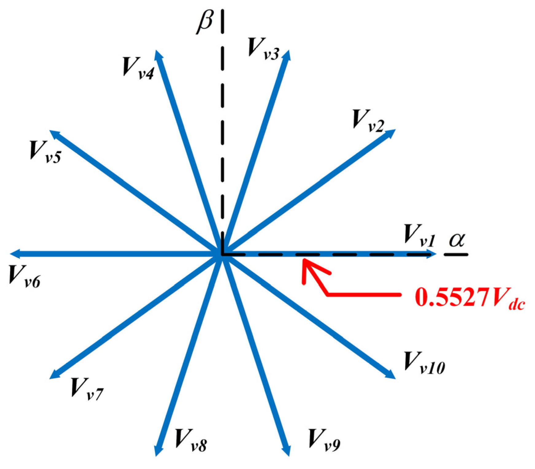
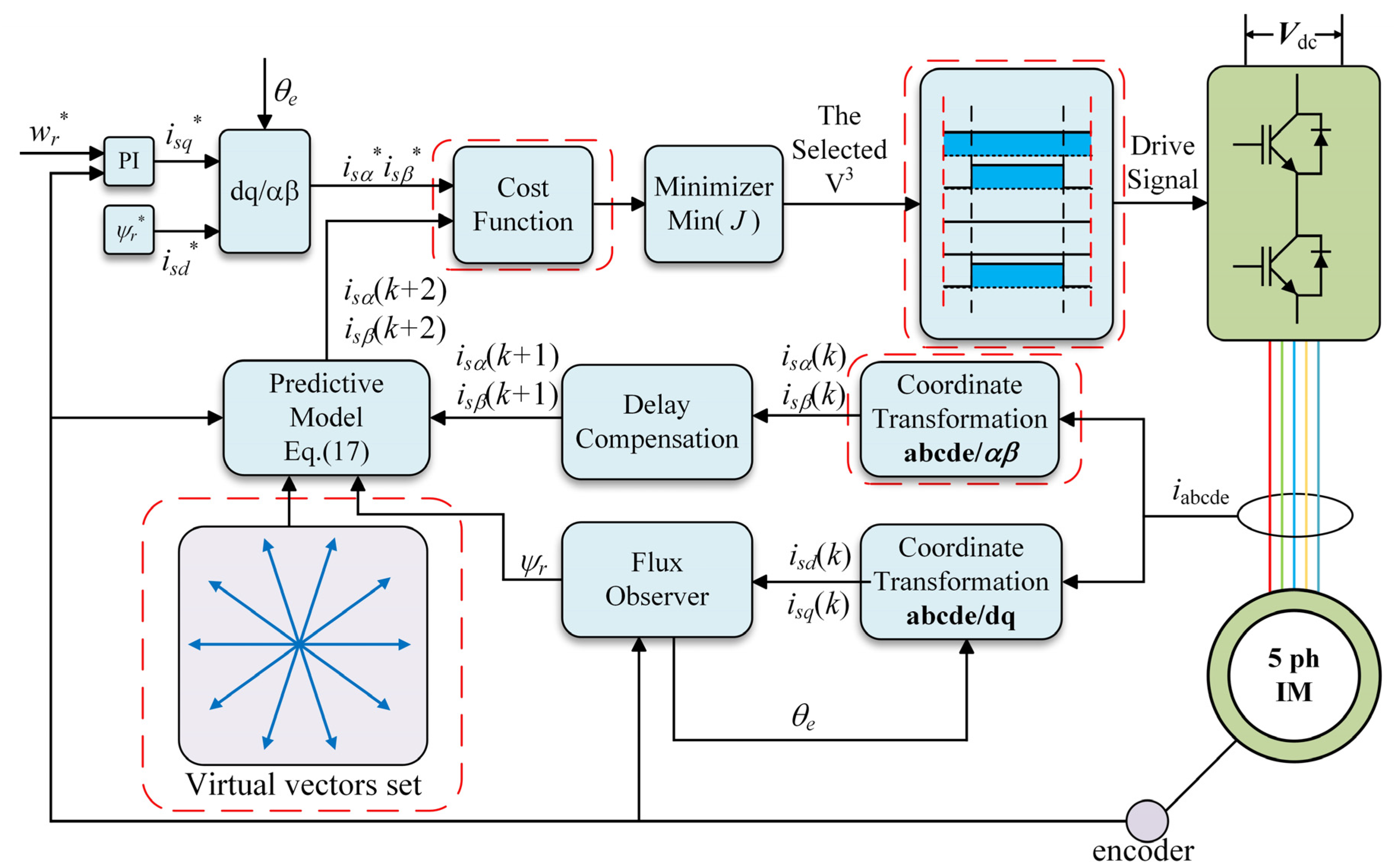
4. Proposed VV-MPCC Schemes

4.1. Prediction Model of Induction Motor

The prediction model can be obtained from the distribution of vectors in Figure 2.

The outermost large vector in the α-β subspace is mapped as the innermost small vector in the x-y subspace, and the median vector in the α-β subspace is still a median vector in the x-y subspace after mapping. However, the direction of small vectors and middle vectors mapped to x-y subspace are opposite to each other.

Since the third harmonic plane current is generated by the third harmonic plane voltage, if the third harmonic plane voltage can be eliminated, the third harmonic plane current can also be eliminated. Therefore, as long as the large vector and the medium vector in the same direction in the fundamental wave plane are combined by a certain ratio, the virtual voltage vector with an average harmonic voltage of 0 in the third harmonic plane can be obtained to achieve the effect of eliminating harmonic current. Figure 4 shows the synthesis process of virtual voltage vector VV₁ by taking medium vector V₁₆ and large vector V₂₅ as examples.

Select the large vector and the medium vector of the fundamental wave space, according to the principle of volt-second balance, the relationship satisfies

$$\left\{\begin{array}{l}0.6472V_{dc}\lambda T_s+0.4V_{dc}(1-\lambda )T_s=\left|V_{VL}\right|T_s\\ 0.6472V_{dc}(1-\lambda )T_s-0.4V_{dc}\lambda T_s=0\end{array}\right.$$

(15)

In Equation (15), |V_VL| represents the amplitude of the synthesized virtual voltage vector, and λT_s represents the action time of large vectors in a single period. From Equation (15), we could achieve:

$$\left\{\begin{array}{c}\left|V_{VL}\right|=0.5527V_{dc}\\ \lambda =0.618\end{array}\right.$$

(16)

According to the above calculation time, the large vector and the medium vector are applied respectively in one cycle. In the fundamental wave space, the new voltage vector synthesized by the large vector and the medium vector in the same direction is called the virtual vector, whose direction is in the same direction with the large and medium vector, and the amplitude is 0.5527V_dc (0.618 × 0.6472V_dc + 0.382 × 0.4V_dc). However, compared with the traditional MPCC, the bus voltage utilization rate is reduced, and the speed regulation range is reduced. Figure 5 shows the distribution of virtual vectors in α-β subspace.

For any virtual vector, the ratio of action time between a large vector and medium vector is constant. No matter whether the virtual vector is synthesized in the order of first large vector followed by a medium vector, or first medium vector followed by a large vector, the waveform symmetry of the virtual vector cannot be guaranteed, so it is difficult to implement in hardware, and it will bring certain high-order harmonics. Therefore, under the condition that the average value of the output voltage remains unchanged, the effective pulse sequence is rearranged according to the principle of centrosymmetry. Figure 6 shows the pulse sequence of VV₁ before and after optimization according to the central symmetry principle, where t₂₅ = λT_s, t₁₆ = (1 − λ)T_s. That is, in a single cycle, the inverter first outputs the switching state of 10,000 with a duration of t₁₆/2, then outputs the switching state of 11,001 with a duration of t_25, and then outputs the switching state of 10,000 with a duration of t₁₆/2. The optimized pulse sequence of the remaining nine virtual vectors is similar to this.

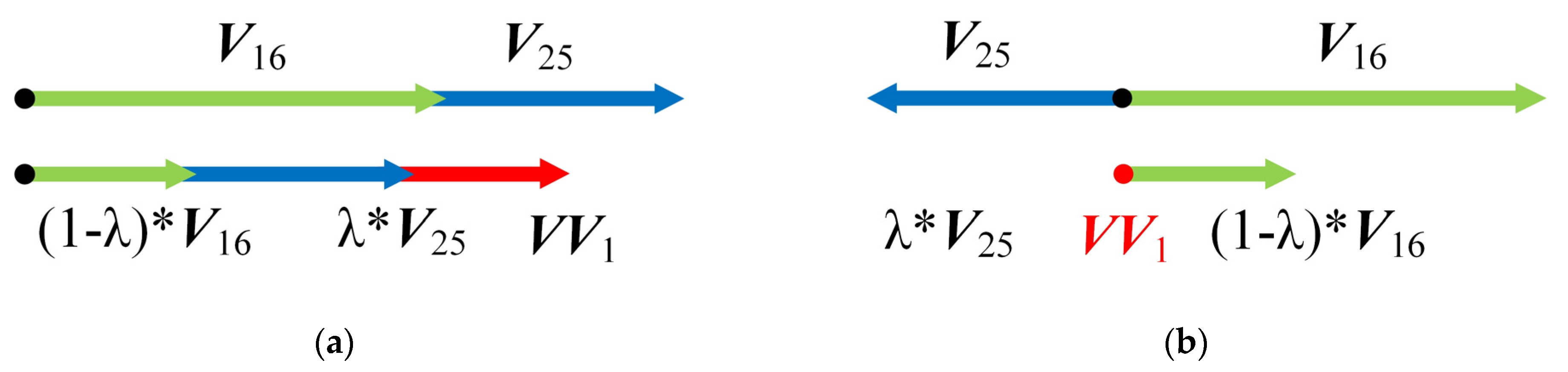
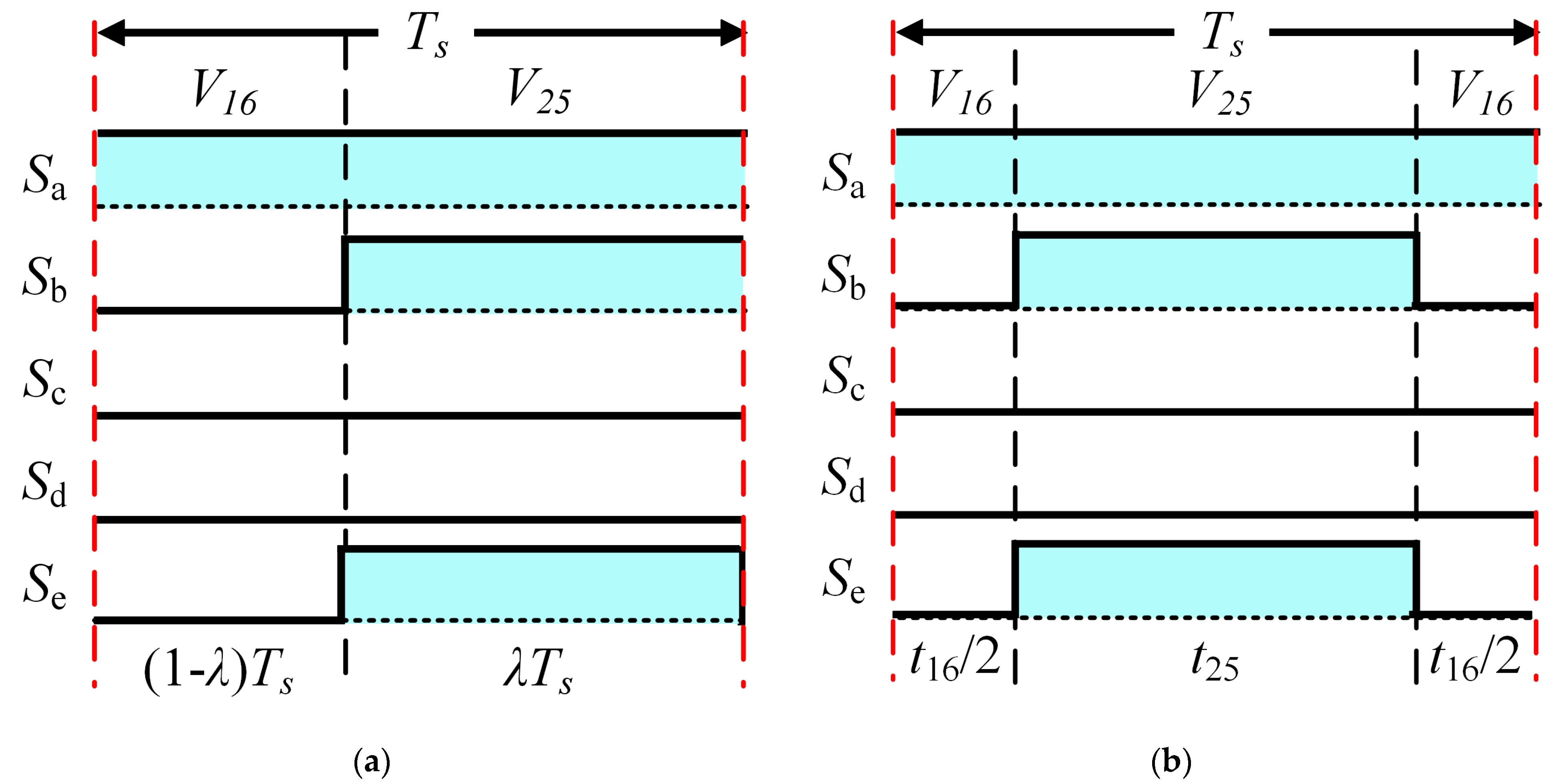
4.2. Cost Function Optimization

When applying virtual vector MPCC, because the third harmonic voltage has been eliminated theoretically, there is no need to predict the harmonic current in the prediction process, and there is no need to include the harmonic current term in the cost function. Therefore, the prediction model and the cost function are simplified. The simplified prediction block diagram is shown in Figure 7. The part in the red dotted line box in the figure shows the difference from the traditional MPCC. The simplified prediction model is:

$$p\cdot X_{\alpha \beta }=A\cdot X_{\alpha \beta }+B\cdot U_{\alpha \beta }$$

(17)

where

$$\begin{gathered} X_{\alpha \beta }={\left[\begin{array}{cccccc}{i}_{s\alpha }& i_{s\beta }& i_{sx}& i_{sy}& {\psi }_{r\alpha }& {\psi }_{r\beta }\end{array}\right]}^T \\ {U}_{\alpha \beta }={\left[\begin{array}{cccc}{u}_{s\alpha }& u_{s\beta }& 0& 0\end{array}\right]}^T \end{gathered}$$

Because the virtual vector is used as the alternative vector set, the number of voltage vectors is also reduced to 10, which reduces the computational burden. The simplified cost function is:

$$J=\left[{(i_{s\alpha }{}^{\ast }-i_{s\alpha })}^2+{(i_{s\beta }{}^{\ast }-i_{s\beta })}^2\right]$$

(18)

Because the average harmonic plane voltage value is 0 only in a single period, and the dead zone effect exists and the motor winding is impossible to make perfectly symmetric, the harmonic plane current will still exist, but the harmonic plane current value will be very small.

5. Simulation Results

In order to prove the effectiveness of the proposed virtual vector MPCC, the motor model and its control system were built in MATLAB/SIMULINK, and the simulation comparison between the proposed method and the traditional MPCC was carried out. The traditional MPCC was written as T-MPC, and the proposed method was denoted as VV-MPC. The parameters of the five-phase induction motor used are shown in

Table 2. Parameters of five-phase induction motor.

Parameter	Symbol/Unit	Value
Stator resistance	Rs[Ω]	1.9
Rotor resistance	Rr[Ω]	3.4
Stator leakage inductance	Lls[mH]	35
Rotor leakage inductance	Llr[mH]	20
Mutual inductance	Lm[mH]	530
Rotational inertia	J[kg·m2]	0.04
Pole pairs	np	2
Rated speed	[r/min]	1500
Rated power	[kW]	2.2

.

5.1. Performance of T-MPC with Different Weighting Factors

The first set of simulations verified the effect of weighting factors on motor dynamic performance and harmonic current suppression. The preset speed of the motor was 500 r/min at 0 s, and the speed command suddenly changed to 1000 r/min at 0.5 s, running with no load. The left side of Figure 8, Figure 9, Figure 10 and Figure 11 represent the operation when the weighting factor was 0.5, and the right side the operation when the weighting factor was 0.1.

Figure 8 shows that the dynamic performance of the motor is similar with different weighting factors. Figure 8 shows that the motor speed is accelerated to 500 r/min within 0.2 s, and then it only requires 0.15 s (0.65 s–0.5 s) to accelerate from 500 r/min to 1000 r/min when it accelerates again. Figure 9 shows that both weighting factors demonstrate fast torque responses, and the torque ripple is smaller when the weighting factor is larger. Figure 10 shows that when the weighting factor is 0.5, the harmonic current is concentrated within ±0.5A, while when the weighting factor is 0.1, the harmonic current is concentrated between ±1A. This indicates that when the weight factor is larger, more attention is paid to the influence of the harmonic plane current and its suppression effect is enhanced, so the amplitude of harmonic current decreases. Figure 11 demonstrates harmonic analysis of phase currents with different weight factors during 1000 r/min operation, and total harmonic distortion (THD) decreases from 23.42% to 18.76%, which further illustrates the improvement effect of larger weighting factors on waveform quality.

This set of simulations shows that although the weighting factor is effective in regulating harmonic currents, since T-MPC only uses a single basic voltage vector in a single switching period, it always generates voltage in the harmonic plane and thus generates large harmonic currents. T-MPC has inherent defects in suppressing harmonic current and improving waveform quality, and it is always unable to obtain better current sinusoids.

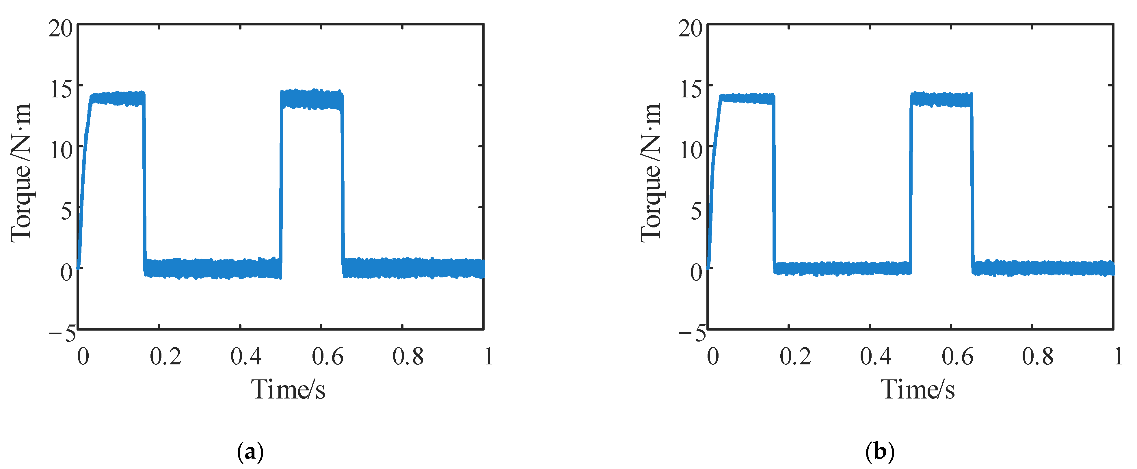
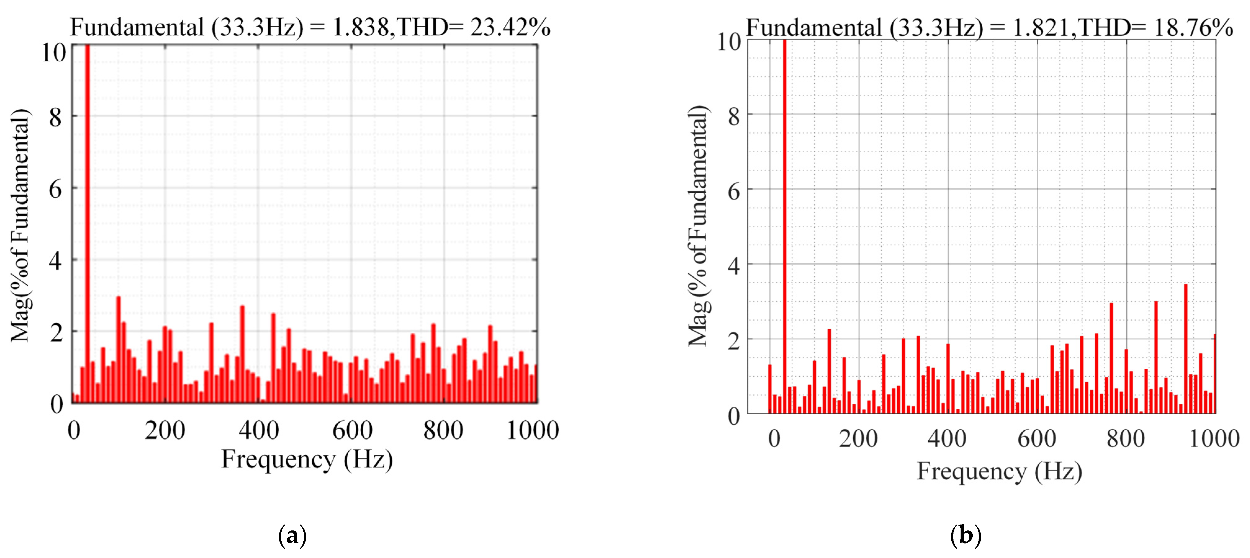
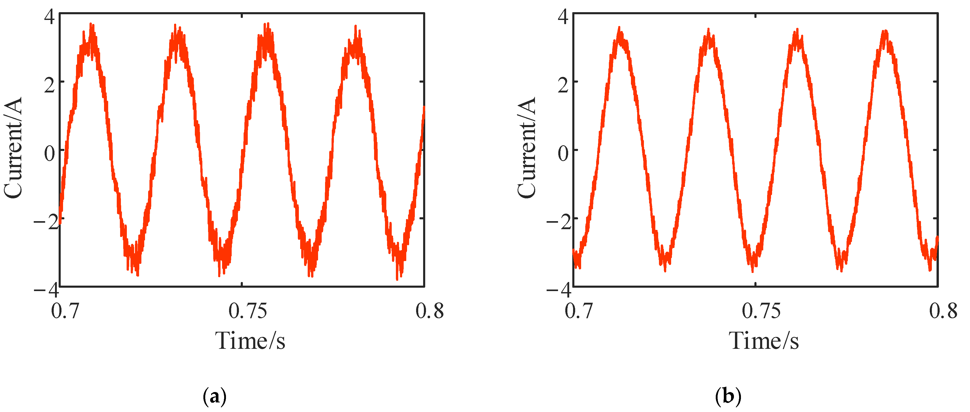
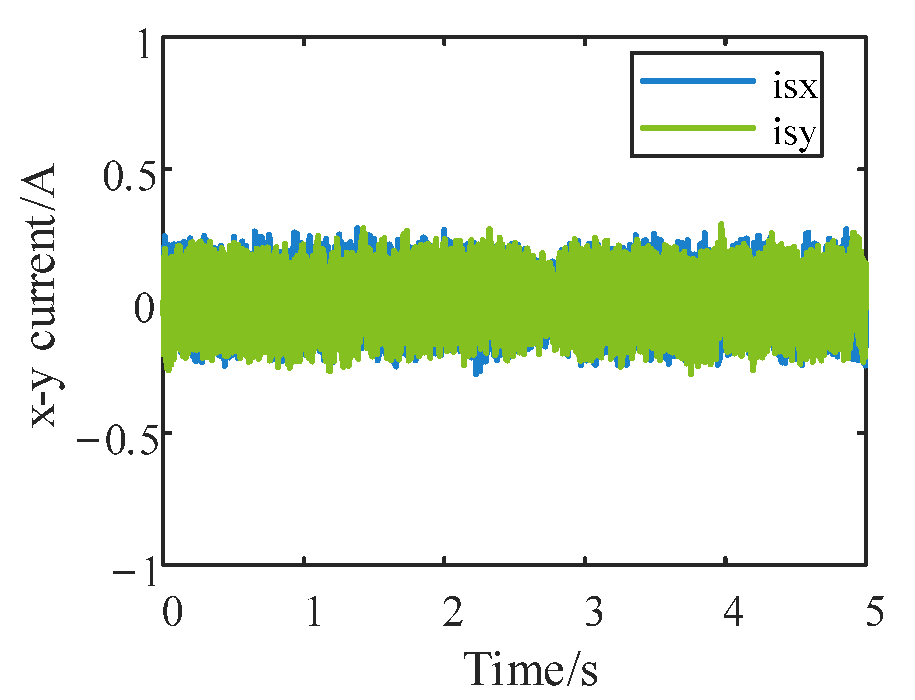
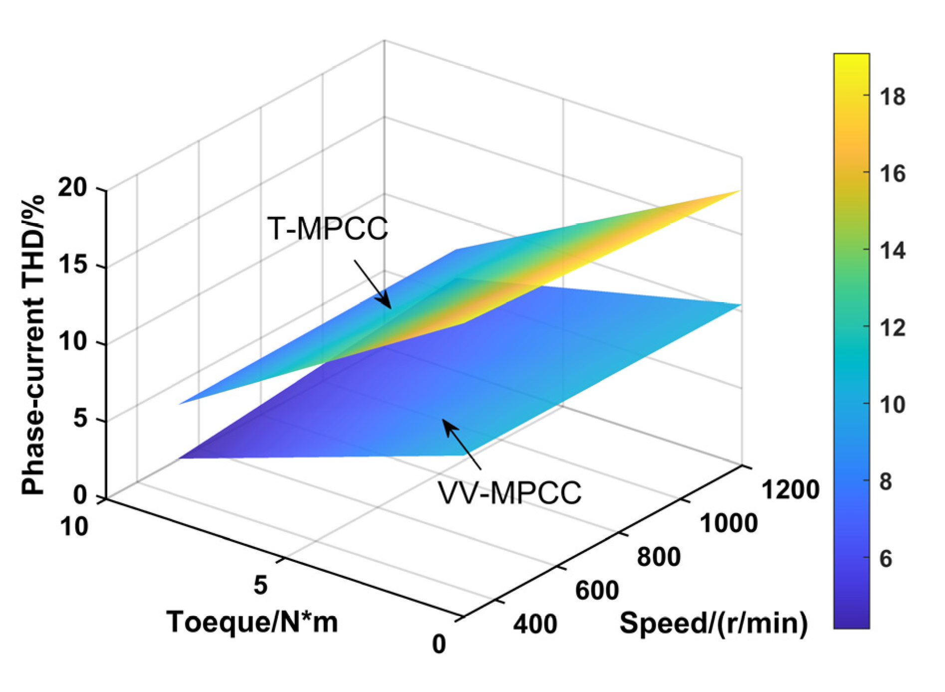
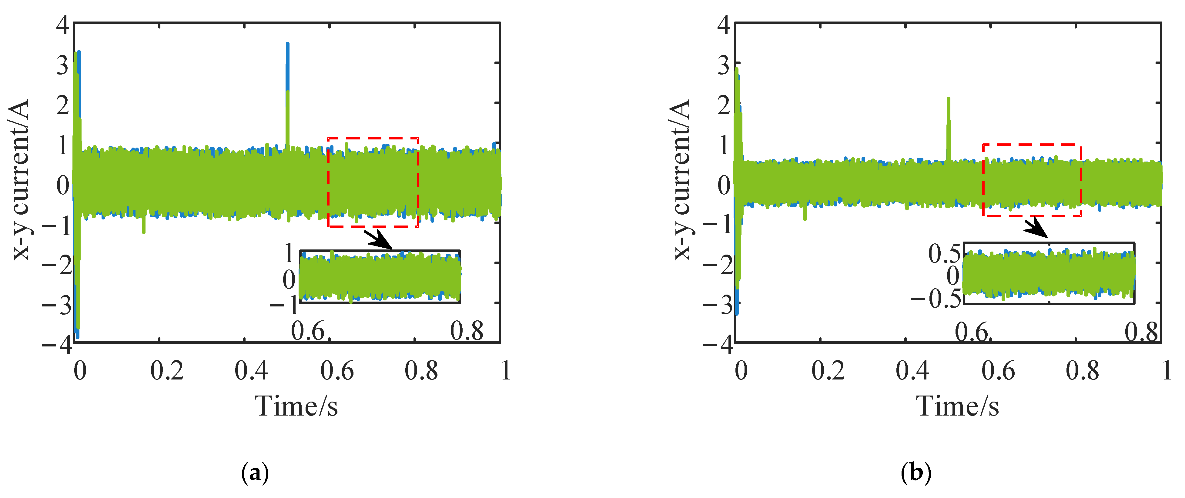
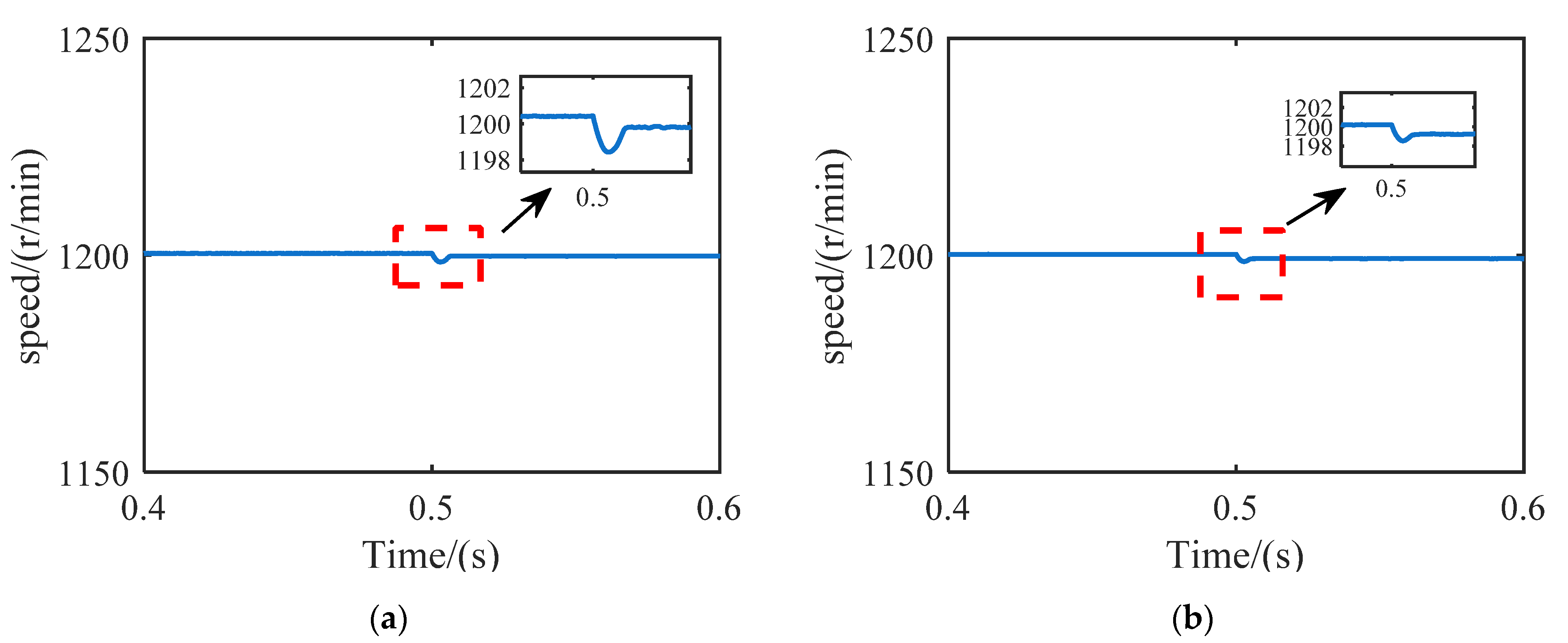
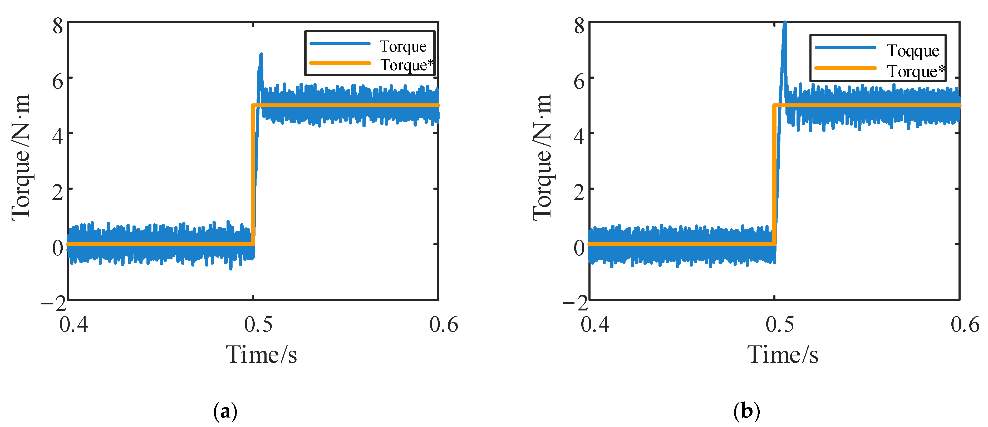
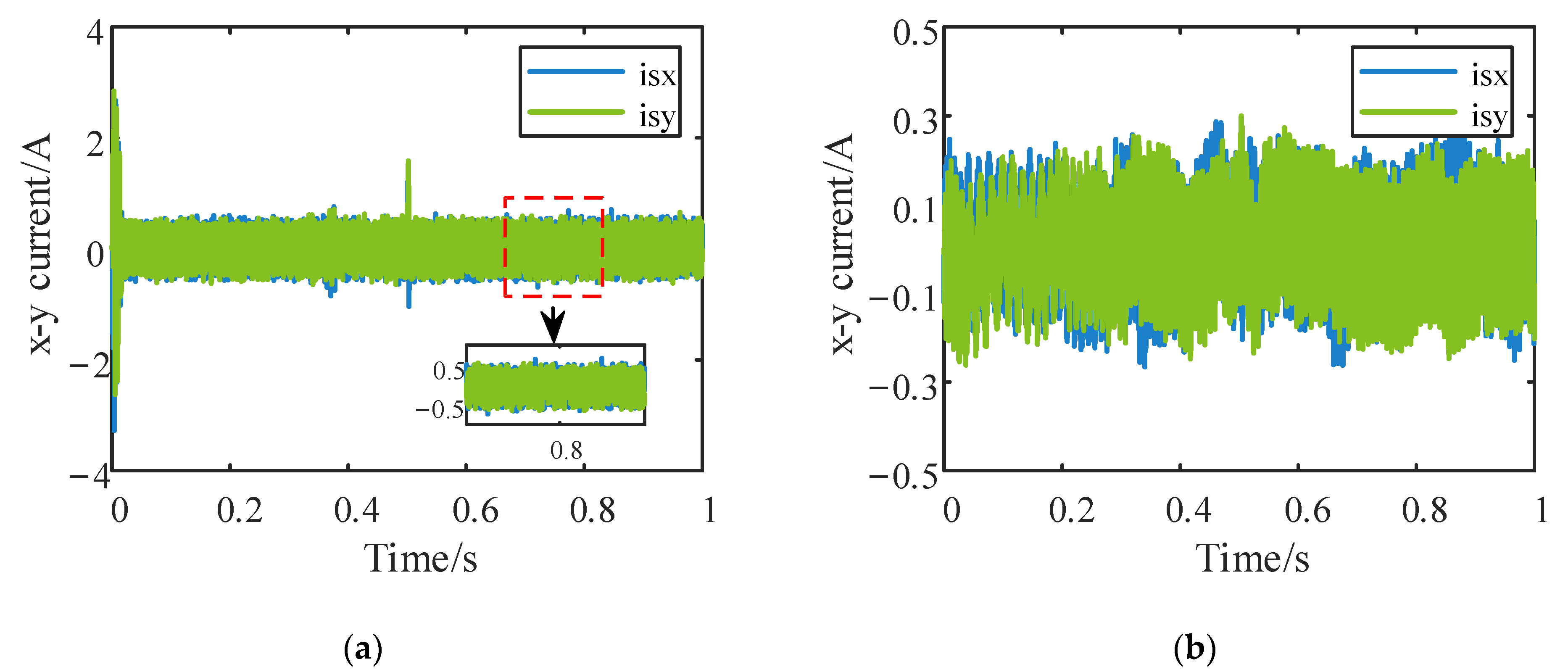
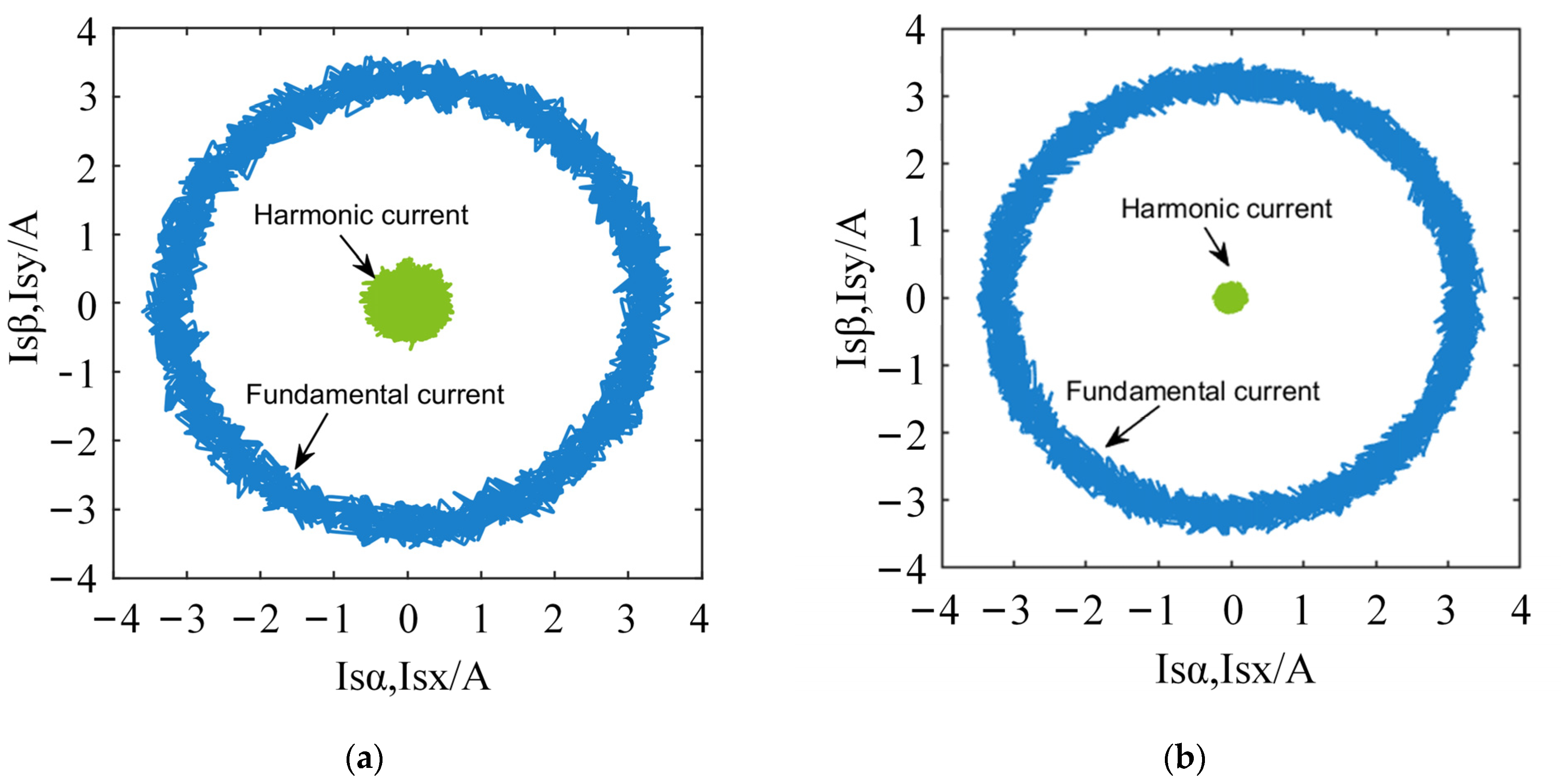
5.2. Performance of Different Control Strategies

The T-MPC and VV-MPC strategies were used, respectively, to make the motors run at 1200 r/min, and a load of 5 N∙m was suddenly applied at 0.5 s.

Figure 12 shows that the motor can run stably at the set speed under different control strategies. When the load is suddenly added, the speed drop is small and the motor can recover previous speed quickly. The superscript * of “Torque” in Figure 13 represents the reference torque. Figure 13 shows that when the load is suddenly added, the output torque of the motor under the two strategies rises rapidly, in which the torque overshoot of VV-MPC is larger and the response is more rapid. Figure 14 shows that the phase current waveform of VV-MPC is less glitchy and the current is more sinusoidal. Figure 15 shows the harmonic currents under different strategies. It can be seen that during the whole loading process, the harmonic currents of VV-MPC are smaller than those of T-MPC under this working condition.

Figure 16 shows the trajectories of fundamental and harmonic plane currents, where the outer ring is the fundamental current trajectory and the inner ring is the harmonic current trajectory. The fundamental current trajectory of VV-MPC is smoother, and the circle formed by the harmonic current has a smaller radius than that of T-MPC, indicating that VV-MPC has an obvious suppressing effect on harmonic currents during steady operation.

This set of simulation shows that after the virtual voltage vectors were adopted, the voltage average value of the harmonic plane was 0, so the current value of the harmonic plane in the VV-MPC method is smaller than that of the T-MPC method. Compared with T-MPC, VV-MPC also has good torque response characteristics when the load is suddenly added, and has a good harmonic current suppression effect when running with load at a steady state.

In order to compare the steady-state performance of the two methods at different speeds, the THD analysis of the phase current of VV-MPC and T-MPC in steady-state operation with load was carried out, respectively.

Table 3. THD analysis of T-MPC and VV-MPC.

Scheme	1200 r/min	750 r/min	300 r/min
T-MPC	10.67%	9.91%	10.77%
VV-MPC	6.65%	5.68%	5.82%

shows the THD analysis of phase current of the two methods at different speeds. It can be seen from Table 3 that, at the same speed, the THD of VV-MPC is about half smaller than that of T-MPC, indicating that VV-MPC has a better suppression effect on harmonic currents and thus obtains a better sinusoidal current. The THD of T-MPC does not change much at different speeds, and the minimum THD is achieved in the medium speed range (750 r/min). VV-MPC can effectively suppress the harmonic current in the whole rate range, and the current quality is better at medium and low speed (300–750 r/min).

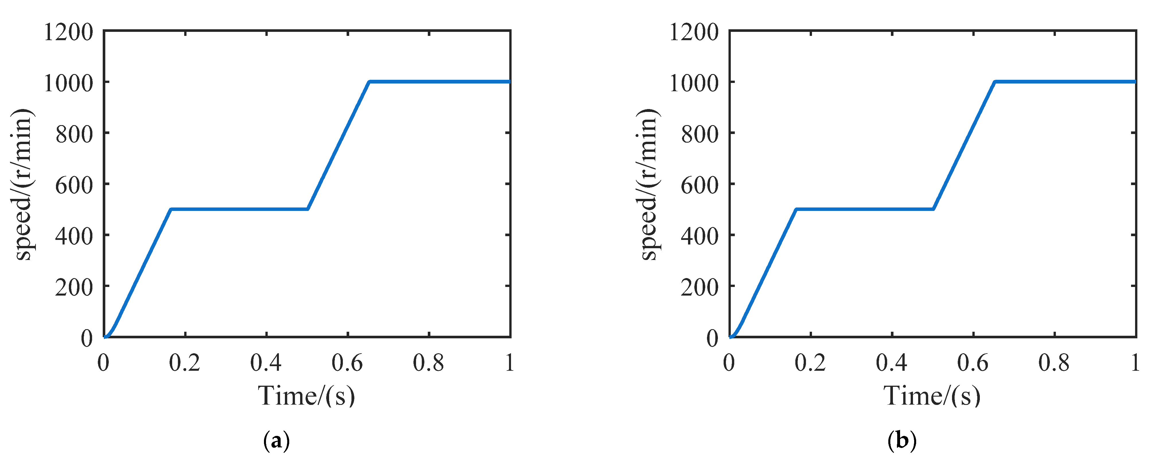
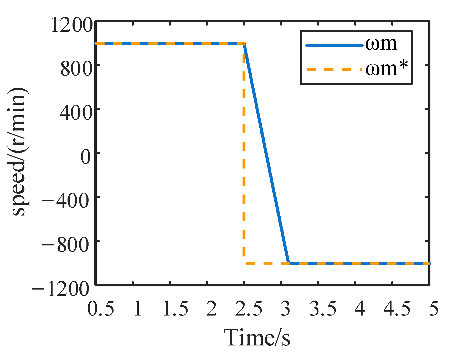
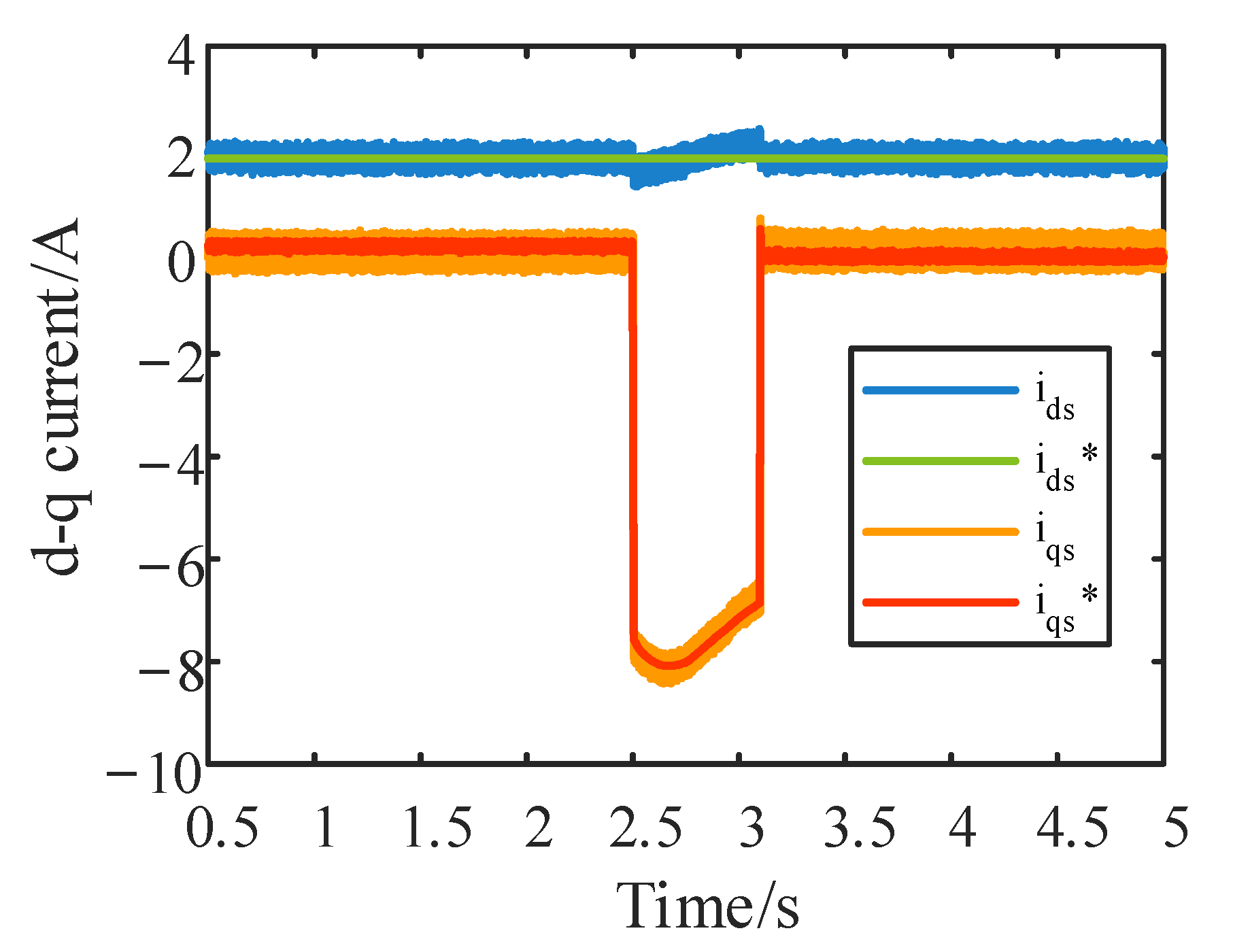
5.3. Forward and Reverse Performance under the Proposed Strategy

In order to further test the dynamic performance of the proposed VV-MPC, the simulation of forward-to- reverse switching under no-load condition was carried out. After acceleration in advance, the motor was stable at 1000 r/min at 0.5 s, and the reference speed became −1000 r/min at 2.5 s. The superscript * of “ωm” in Figure 17 represents the reference speed. Figure 17 shows that the actual speed of the motor quickly tracks the reference speed and runs stably at −1000 r/min after 0.6 s. The d-q axis current and its reference value during the whole switching period are shown in Figure 18. The superscript * in Figure 18 represents the reference d-axis current and reference q-axis current. It can be seen that the reference current of the d-axis keeps constant, while the actual current value of the d-axis fluctuates more than during the steady-state operation only during the conversion process of 2.5 s–3.1 s, but the reference value can still be tracked. When the speed reference command changes, in order to force the motor to decelerate rapidly and reverse, the reference value of the q-axis current quickly changes to −8A, and the actual value is immediately tracked, which reflects that it still has good dynamic performance in the extreme case of forward and reverse switching. Figure 19 shows that during the entire operation process, the harmonic current is always maintained between −0.3A and 0.3A, and the harmonic suppression ability is not affected by the working conditions.

5.4. The Performance of the Proposed Strategy under All Operating Conditions

In order to compare the performance differences between the proposed VV-MPC and T-MPC at different speeds and different loads, the speed values used were 300 r/min, 600 r/min, 900 r/min, 1200 r/min, and the loads used were 2 N·m, 4 N·m, 6 N·m, 8 N·m, 10 N·m. Multiple sets of simulations were performed, and the results are displayed in three-dimensional diagrams as shown in Figure 20 and Figure 21.

Figure 20 shows that the THD-plane of VV-MPC and T-MPC does not overlap at full speed and under full working conditions, which fully shows that VV-MPC can effectively suppress harmonic current at any speed and load compared with T-MPC. At the same time, it can be seen that for these two control strategies, the THD of the motor with light load is greater than that of the motor with heavy load, indicating that the waveform quality of the two strategies under load is improved compared with that of no load. With the same load, THD does not change much with the increase of the motor speed, indicating that the speed has little influence on the phase current THD of the motor.

Figure 21 shows that the switching frequency of T-MPC changes slowly and does not change greatly with the change of load. The switching frequency at low speed is slightly lower than that at high speed. At 300 r/min and no load, the minimum switching frequency is 1.4 kHz and the maximum is 1.8 kHz at 1200 r/min and no load. This indicates that the same voltage vector will be used for a long period of time, which means that the switching device will not act. The switching frequency of VV-MPC varies greatly with the speed. The switching frequency is low at low speeds, about 2.1 kHz at 300 r/min, and high at high speeds, about 5 kHz at 1200 r/min. It can be speculated that when the speed increases, the stator current frequency also increases, so that the switching frequency increases. For these two strategies, the control frequency is set to 10 kHz, and the switching frequency of VV-MPC, which has the highest switching frequency, is only about 5 kHz, indicating that the MPC has the characteristic of low switching frequency.

6. Conclusions

Although T-MPC still has good dynamic performance when extended to multiphase systems, it lacks effective suppression of harmonic plane currents. The single switching state used in T-MPC will inevitably bring the problem of high harmonic plane currents. In this paper, ten new virtual vectors were synthesized from the large and medium vectors in the same direction in α-β space according to the fixed ratio by using the vector distribution characteristics of five-phase inverter. Taking the virtual vector set as the alternative vector set, the VV-MPC method based on the virtual vector set was proposed and applied to a five-phase induction motor. The advantages of the proposed VV-MPC can be summarized as follows:

(1) Compared with the traditional method, the proposed method has excellent dynamic performance, and the harmonic plane current value is greatly reduced, so as to achieve the purpose of suppressing harmonic current, reducing harmonic loss and improving power quality.

(2) Due to the reduction of the number of vectors in the alternative vector set, the calculation amount of MPC in each cycle is reduced.

(3) In the proposed method, the theoretical average value of the harmonic plane voltage is 0, so there is no need to predict the harmonic plane currents in the prediction process, the weighting factor is omitted, and the prediction model is simplified.

References

1. Chan, C.C. The State of the Art of Electric, Hybrid, and Fuel Cell Vehicles. Proc. IEEE 2007, 95, 704–718. [Google Scholar] [CrossRef]
2. Sun, X.; Jin, Z.; Wang, S.; Yang, Z.; Li, K.; Fan, Y.; Chen, L. Performance Improvement of Torque and Suspension Force for a Novel Five-Phase BFSPM Machine for Flywheel Energy Storage Systems. IEEE Trans. Appl. Supercond. 2019, 29, 5–9. [Google Scholar] [CrossRef]
3. Chau, K.T.; Chan, C.C.; Liu, C. Overview of Permanent-Magnet Brushless Drives for Electric and Hybrid Electric Vehicles. IEEE Trans. Ind. Electron. 2008, 55, 2246–2257. [Google Scholar] [CrossRef]
4. Frieske, B.; Kloetzke, M.; Mauser, F. Trends in Vehicle Concept and Key Technology Development for Hybrid and Battery Electric Vehicles. World Electr. Veh. J. 2013, 6, 9–20. [Google Scholar] [CrossRef]
5. Bojoi, R.; Rubino, S.; Tenconi, A.; Vaschetto, S. Multiphase Electrical Machines and Drives: A Viable Solution for Energy Generation and Transportation Electrification. In Proceedings of the 2016 International Conference and Exposition on Electrical and Power Engineering (EPE), Iasi, Romania, 20–22 October 2016; pp. 632–639. [Google Scholar] [CrossRef]
6. Cao, W.; Mecrow, B.C.; Atkinson, G.J.; Bennett, J.W.; Atkinson, D.J. Overview of Electric Motor Technologies Used for More Electric Aircraft (MEA). IEEE Trans. Ind. Electron. 2012, 59, 3523–3531. [Google Scholar] [CrossRef]
7. Tao, T.; Zhao, W.; He, Y.; Cheng, Y.; Saeed, S.; Zhu, J. Enhanced Fault-Tolerant Model Predictive Current Control for a Five-Phase PM Motor with Continued Modulation. IEEE Trans. Power Electron. 2021, 36, 3236–3246. [Google Scholar] [CrossRef]
8. Fnaiech, M.A.; Betin, F.; Capolino, G.-A.; Fnaiech, F. Fuzzy Logic and Sliding-Mode Controls Applied to Six-Phase Induction Machine with Open Phases. IEEE Trans. Ind. Electron. 2010, 57, 354–364. [Google Scholar] [CrossRef]
9. Zheng, L.; Fletcher, J.E.; Williams, B.W.; He, X. Dual-Plane Vector Control of a Five-Phase Induction Machine for an Improved Flux Pattern. IEEE Trans. Ind. Electron. 2008, 55, 1996–2005. [Google Scholar] [CrossRef]
10. Diana, M.; Guglielmi, P.; Vagati, I.A. Very Low Torque Ripple Multi-3-Phase Machines. In Proceedings of the IECON 2016—42nd Annual Conference of the IEEE Industrial Electronics Society, Florence, Italy, 24–27 October 2016; IEEE: Piscataway, NJ, USA, 2016; pp. 1750–1755. [Google Scholar]
11. Li, G.; Hu, J.; Li, Y.; Zhu, J. An Improved Model Predictive Direct Torque Control Strategy for Reducing Harmonic Currents and Torque Ripples of Five-Phase Permanent Magnet Synchronous Motors. IEEE Trans. Ind. Electron. 2019, 66, 5820–5829. [Google Scholar] [CrossRef]
12. Cortés, P.; Kazmierkowski, M.P.; Kennel, R.M.; Quevedo, D.E.; Rodriguez, J. Predictive Control in Power Electronics and Drives. IEEE Trans. Ind. Electron. 2008, 55, 4312–4324. [Google Scholar] [CrossRef]
13. Elmorshedy, M.F.; Xu, W.; El-Sousy, F.F.M.; Islam, M.R.; Ahmed, A.A. Recent Achievements in Model Predictive Control Techniques for Industrial Motor: A Comprehensive State-of-the-Art. IEEE Access 2021, 9, 58170–58191. [Google Scholar] [CrossRef]
14. Martinez, J.C.R.; Kennel, R.M.; Geyer, T. Model Predictive Direct Current Control. In Proceedings of the 2010 IEEE International Conference on Industrial Technology, Vina del Mar, Chile, 14–17 March 2010; IEEE: Piscataway, NJ, USA, 2010; pp. 1808–1813. [Google Scholar]
15. Iqbal, A.; Alammari, R.; Mosa, M.; Abu-Rub, H. Finite Set Model Predictive Current Control with Reduced and Constant Common Mode Voltage for a Five-Phase Voltage Source Inverter. In Proceedings of the 2014 IEEE 23rd International Symposium on Industrial Electronics (ISIE), Istanbul, Turkey, 1–4 June 2014; pp. 479–484. [Google Scholar] [CrossRef]
16. Stolze, P.; Tomlinson, M.; Kennel, R.; Mouton, T. Heuristic Finite-Set Model Predictive Current Control for Induction Machines. In Proceedings of the 2013 IEEE ECCE Asia Downunder—5th IEEE Annual International Energy Convers, Melbourne, VIC, Australia, 3–6 June 2013; pp. 1221–1226. [Google Scholar] [CrossRef]
17. Xue, Y.; Meng, D.; Zhao, Z.; Zhao, L.; Diao, L. Model Predictive Current Control in the Stationary Coordinate System for a Three-Phase Induction Motor Fed by a Two-Level Inverter. In Proceedings of the 2019 IEEE International Symposium on Predictive Control of Electrical Drives and Power Electronics (PRECEDE), Quanzhou, China, 31 May–2 June 2019; IEEE: Piscataway, NJ, USA, 2019; pp. 1–5. [Google Scholar]
18. Kousalya, V.; Rai, R.; Singh, B. Predictive Torque Control of Induction Motor for Electric Vehicle. In Proceedings of the 2020 IEEE Transportation Electrification Conference & Expo (ITEC), Chicago, IL, USA, 23–26 June 2020; IEEE: Piscataway, NJ, USA, 2020; pp. 890–895. [Google Scholar]
19. Rivera, M.; Riveros, J.A.; Rodriguez, C.; Wheeler, P. Field-Oriented Control with a Predictive Current Strategy of an Induction Machine Fed by a Two-Level Voltage Source Inverter. In Proceedings of the 2021 IEEE International Conference on Automation/XXIV Congress of the Chilean Association of Automatic Control (ICA-ACCA), Valparaíso, Chile, 22–26 March 2021. [Google Scholar] [CrossRef]
20. Lim, C.S.; Levi, E.; Jones, M.; Abdul Rahim, N.; Hew, W.P. Experimental Evaluation of Model Predictive Current Control of a Five-Phase Induction Motor Using All Switching States. In Proceedings of the 2012 15th International Power Electronics and Motion Control Conference (EPE/PEMC), Novi Sad, Serbia, 4–6 September 2012; pp. 1–7. [Google Scholar] [CrossRef]
21. Xue, C.; Song, W.; Feng, X. Model Predictive Current Control Schemes for Five-Phase Permanent-Magnet Synchronous Machine Based on SVPWM. In Proceedings of the 2016 IEEE 8th International Power Electronics and Motion Control Conference (IPEMC-ECCE Asia), Hefei, China, 22–26 May 2016; pp. 648–653. [Google Scholar] [CrossRef]
22. Lim, C.S.; Levi, E.; Jones, M.; Rahim, N.A.; Hew, W.P. FCS-MPC-Based Current Control of a Five-Phase Induction Motor and Its Comparison with PI-PWM Control. IEEE Trans. Ind. Electron. 2014, 61, 149–163. [Google Scholar] [CrossRef]
23. Bermúdez, M.; Martín, C.; González-Prieto, I.; Durán, M.J.; Arahal, M.R.; Barrero, F. Predictive Current Control in Electrical Drives: An Illustrated Review with Case Examples Using a Five-phase Induction Motor Drive with Distributed Windings. IET Electr. Power Appl. 2020, 14, 1291–1310. [Google Scholar] [CrossRef]
24. Cortes, P.; Wilson, A.; Kouro, S.; Rodriguez, J.; Abu-Rub, H. Model Predictive Control of Multilevel Cascaded H-Bridge Inverters. IEEE Trans. Ind. Electron. 2010, 57, 2691–2699. [Google Scholar] [CrossRef]
25. Duran, M.J.; Prieto, J.; Barrero, F.; Toral, S. Predictive Current Control of Dual Three-Phase Drives Using Restrained Search Techniques. IEEE Trans. Ind. Electron. 2011, 58, 3253–3263. [Google Scholar] [CrossRef]
26. Zheng, L.; Fletcher, J.E.; Williams, B.W.; He, X. A Novel Direct Torque Control Scheme for a Sensorless Five-Phase Induction Motor Drive. IEEE Trans. Ind. Electron. 2011, 58, 503–513. [Google Scholar] [CrossRef]
27. Bermudez, M.; Gonzalez-Prieto, I.; Barrero, F.; Guzman, H.; Duran, M.J.; Kestelyn, X. Open-Phase Fault-Tolerant Direct Torque Control Technique for Five-Phase Induction Motor Drives. IEEE Trans. Ind. Electron. 2017, 64, 902–911. [Google Scholar] [CrossRef]
28. Romero, C.; Delorme, L.; Gonzalez, O.; Ayala, M.; Rodas, J.; Gregor, R. Algorithm for Implementation of Optimal Vector Combinations in Model Predictive Current Control of Six-Phase Induction Machines. Energies 2021, 14, 3857. [Google Scholar] [CrossRef]
29. Gonzalez-Prieto, I.; Duran, M.J.; Aciego, J.J.; Martin, C.; Barrero, F. Model Predictive Control of Six-Phase Induction Motor Drives Using Virtual Voltage Vectors. IEEE Trans. Ind. Electron. 2018, 65, 27–36. [Google Scholar] [CrossRef]
30. Ryu, H.M.; Kim, J.H.; Sul, S.K. Analysis of Multiphase Space Vector Pulse-Width Modulation Based on Multiple d-q Spaces Concept. IEEE Trans. Power Electron. 2005, 20, 1364–1371. [Google Scholar] [CrossRef]
31. Wang, F.; Li, S.; Mei, X.; Xie, W.; Rodriguez, J.; Kennel, R.M. Model-Based Predictive Direct Control Strategies for Electrical Drives: An Experimental Evaluation of PTC and PCC Methods. IEEE Trans. Ind. Inform. 2015, 11, 671–681. [Google Scholar] [CrossRef]
32. Cortes, P.; Rodriguez, J.; Silva, C.; Flores, A. Delay Compensation in Model Predictive Current Control of a Three-Phase Inverter. IEEE Trans. Ind. Electron. 2012, 59, 1323–1325. [Google Scholar] [CrossRef]
Figure 1. Diagram of five-phase induction motor system.
Processes 10 01925 g001
Figure 2. Voltage space vectors in two subspaces. (a) α-β subspace. (b) x-y subspace.
Processes 10 01925 g002
Figure 3. Traditional FCS-MPCC scheme for a five-phase IM (Induction Motor) drive.
Processes 10 01925 g003
Figure 4. Schematic of virtual voltage vector synthesis (a) α-β subspace; (b) x-y subspace.
Processes 10 01925 g004
Figure 5. Virtual voltage vectors in α-β subspace.
Processes 10 01925 g005
Figure 6. Schematic diagram of the virtual vector implementation method (VV1). (a) Initial mode; (b) Symmetrical mode.
Processes 10 01925 g006
Figure 7. Proposed FCS-MPCC with VVs scheme for a five-phase IM drive.
Processes 10 01925 g007
Figure 8. Speed performance of T-MPC scheme with different weighing factors at same sampling frequency (10 kHz). (a) Wxy = 0.1; (b) Wxy = 0.5.
Processes 10 01925 g008
Figure 9. Torque performance of T-MPC scheme with different weighing factors at same sampling frequency (10 kHz). (a) Wxy = 0.1; (b) Wxy = 0.5.
Processes 10 01925 g009
Figure 10. Harmonic currents of T-MPC scheme with different weighing factors at same sampling frequency (10 kHz). (a) Wxy = 0.1; (b) Wxy = 0.5.
Processes 10 01925 g010
Figure 11. Total harmonic distortion (THD) performance of T-MPC scheme with different weighing factors at same sampling frequency (10 kHz). (a) Wxy = 0.1; (b) Wxy = 0.5.
Processes 10 01925 g011
Figure 12. Performance of speed when loaded for two FCS-MPCC schemes at same sampling frequency (10 kHz). (a) T-MPC; (b) VV-MPC.
Processes 10 01925 g012
Figure 13. Performance of torque when loaded for two FCS-MPCC schemes at same sampling frequency (10 kHz). (a) T-MPC; (b) VV-MPC.
Processes 10 01925 g013
Figure 14. Performance of phase current in steady-state for two FCS-MPCC schemes at same sampling frequency (10 kHz). (a) T-MPC; (b) VV-MPC.
Processes 10 01925 g014
Figure 15. Performance of harmonic current for two FCS-MPCC schemes at same sampling frequency (10 kHz). (a) T-MPC; (b) VV-MPC.
Processes 10 01925 g015
Figure 16. Performance of current trajectories of fundamental and harmonic currents for two FCS-MPCC schemes at same sampling frequency (10 kHz). (a) T-MPC; (b) VV-MPC.
Processes 10 01925 g016
Figure 17. Performance of speed when used VV-MPC in speed reversal simulation.
Processes 10 01925 g017
Figure 18. Performance of d-q current tracking error when used VV-MPC in speed reversal simulation.
Processes 10 01925 g018
Figure 19. Performance of harmonic current when used VV-MPC in speed reversal simulation.
Processes 10 01925 g019
Figure 20. Effects of torque and speed on phase current.
Processes 10 01925 g020
Figure 21. Effects of torque and speed on switching frequency.
Processes 10 01925 g021