Recurrent Neural Network-Based Temperature Control System Weight Pruning Based on Nonlinear Reconstruction Error

Abstract

Recurrent Neural Networks (RNNs) have been widely applied in various fields. However, in real-world application, because most devices like mobile phones are limited to the storage capacity when processing real-time information, an over-parameterized model always slows down the system speed and is not suitable to be employed. In our proposed temperature control system, the RNN-based control model processes the real-time temperature signals. It is necessary to compress the trained model with acceptable loss of control performance for further implementation in the actual controller when the system resource is limited. Inspired by the layer-wise neuron pruning method, in this paper, we apply the nonlinear reconstruction error (NRE) guided layer-wise weight pruning method on the RNN-based temperature control system. The control system is established based on MATLAB/Simulink. In order to compress the model size to save the memory capacity of temperature controller devices, we first prove the validity of the proposed reference-model (ref-model) guided RNN model for real-time online data processing on an actual temperature object; relative experiments are implemented based on a digital signal processor. On this basis, we then verified the NRE guided layer-wise weight pruning method on the well-trained temperature control model. Compared with the classical pruning method, experiment results indicate that the pruned control model based on NRE guided layer-wise weight pruning can effectively achieve the high accuracy at targeted sparsity of the network.

1. Introduction

Temperature control plays an important role in food production, packaging machine and many other manufacturing processes. Efficient and precise temperature control is the key for ensuring high quality of production [1,2]. Until now, the design and implementation of a PID controller and the model predictive control strategy have been popular in temperature control or weather forecasts [3,4]. However, due to the complex nonlinear control object in industry, the PID controller always requires more re-tuning and has difficulty in achieving desired control performance for changing conditions [5]. The model predictive control commonly handles the quadratic programming problem for those complex multivariable systems in the industrial process control [6]. However, in order to improve control performance, more complex physical models or nonlinear optimization solvers are commonly required. In addition, its physical model and control parameters do not adapt to changes in the controlled object and operating environment. In recent years, with the development of machine learning, from support vector machine to artificial neural network [7,8], they have been more and more widely adopted for solving practical problems. However, although support vector machine can be used to deal with nonlinear and local minimum problems, it is not suitable for dealing with large-scale data problems. On the other hand, the conventional artificial neural network has the advantage of self-learning ability and can approximate the nonlinear function easily, but it also cannot learn the correlation in the sequence data effectively and the time feature needs to be selected artificially, which affects the actual prediction results [9]. Nowadays, with the development of deep learning, especially the emergence of the recurrent neural network, it can learn the dependence relationship of time series more accurately [10]. Compared to the common deep neural network, it solves the problem that time features need to be extracted manually and avoid breaking the time sequence of data. In fact, it is a type of neural network with feedback loops within the hidden layer that can effectively handle the state for each time step. Unlike the conventional feedforward neural networks, its current processing of the input data relays on the outputs of the previous time steps; meanwhile, its current state is transformed as the input value for the next state [11,12]. Benefitting from its specific structure, it has been applied in many real applications, such as time-series market data processing, text generation and machine translation [13,14,15,16]. Considering these advantages, the RNN model can be as a powerful tool, adopted to our temperature control system to process the time series data for achieving desired control performance.

However, with rapid development and growing requirements on deep learning, models of large sizes are required for capturing the features of the controlled object. Large numbers of connection parameters are contained and the consumption of computing resources is also expanded. These models with large size of parameters affect the device running speed and require a large amount of storage space during inference, which largely limits further application and promotion of deep neural networks for real application in industry [17,18,19]. At present, many studies have demonstrated that there are a large number of redundant connection parameters, and only a small portion of them actually contribute to the final performance of control systems [20,21,22]. That means, even if only a small portion of the weight parameters is retained from the original model after trimming, they can also be trained to achieve similar performance to the original network. For accelerating the deep neural network (DNN) model, neural network pruning is an effective method proposed to reduce the number of parameters and computations by removing unimportant connections of the entire neural network (the corresponding values are equal to 0). The standard pruning method proposed earlier can be mainly summarized as follows: Firstly, an over-parameterized model was trained, then the connection parameters of the pre-trained model were cut off according to certain criteria, and finally the trimmed model was fine tuned to recover lost precision of the model as much as possible [23,24,25]. Until the system performance meets the requirement, the pruning and fine-tuning processes are usually performed iteratively. Ideally, pruning method helps the model find the fewest number of parameters for each layer while the existing connections can express the optimal performance after pruning. Moreover, some studies also suggest that pruning technologies sometimes can get higher accuracy for removing a small amount of connections [26].

The type of pruning structure can be mainly divided into structured pruning and unstructured pruning according to different removed objects, respectively, representing the entire set of neurons (channels or filters in convolutional neural networks) and individual connections. The former combined with higher sparsity that discards the neurons directly thus holds the obvious speed and storage advantages under the current hardware conditions [27,28,29]. On the other hand, its clear disadvantage is its large sparsity, which makes it much easier to cause great damage to the accuracy. For a DNN model applied in the industrial application, a pruned structure needs to maintain the accuracy as the original as much as possible; otherwise there will be great damage to the performance of the control system. Until now, various pruning methods have been proposed and outperformed on the existing standard models for image datasets, such as the experiments on AlexNet and VGGNet on ImageNet; different levels of connection parameters are removed by taking appropriate approaches [30,31,32]. Despite these pruning methods compressing the DNN models with little or almost no accuracy loss, most studies only focus on convolutional neural networks (CNNs) for pruning channels, block and filter [33,34,35], which is not suitable for the RNN model structure. Different from the structural pruning in common feedforward network models, directly removing an entire row or column values from weight matrices will lead to the problem that the feature dimensions do not match and produce invalid units. Meanwhile, while the unstructured pruning tends to be together with some computation libraries or hardware, it also ensures the higher accuracy that is quite important in industrial application. More recently, relative studies based on GPU kernels for speeding up unstructured pruning operations have also been proposed [36,37,38]. Hence, we consider the effective weight pruning method for our proposed temperature control system.

In previous work, we implemented an RNN-based model for processing sequential data of the temperature control system [39]. It is combined with a pre-designed reference model and simulation experiments were conducted with MATLAB software. The simulation results proved the proposed Reference-model-based RNN (RM-RNN) control system can achieve the desired performance compared to the conventional control methods. In this paper, we first apply our model based on an actual temperature control object in the experiment environment, then analyze the response characteristics of the temperature system to validate the reasonability and validity of the trained model. On this basis, this is enacted for further effective compression of the pre-trained model in a high pruning rate and simultaneous elimination of the accuracy loss of our temperature control system. Inspired by the layer-wise neuron pruning method [40,41,42], we adopt the layer-wise weight pruning based on minimizing nonlinear reconstruction error (values after nonlinear functions) to get the optimal performance at the given sparsity ratio for our proposed RM-RNN temperature control model.

This paper is mainly organized as follows. In Section 2, our proposed RM-RNN control model for a temperature control system is generally reviewed. The control structure is introduced briefly for pruning experiments. Meanwhile, the experimental results of the proposed control approach for temperature control system are described and the stability and anti-disturbance capacity of the control system are analyzed in the actual utilization. On this basis, the layer-wise nonlinear reconstruction error pruning method is introduced and implemented concerning the pre-trained RNN model in Section 3. Finally, the conclusions and discussion are included in Section 4.

2. Materials and Methods

In order to verify the validity of the proposed RM-RNN temperature control method, we firstly review the framework that was implemented in the previous simulation experiments, concerning which the control object function is derived from an actual temperature controlled object. In this section, the experiments with the identified temperature model are carried out to bring the feasibility and effectiveness of the proposed control model into conformity.

2.1. Framework of the Temperature Control System

2.1.1. The Proposed RNN-Based Temperature Control System

The framework of the overall temperature control system is shown in Figure 1. It consists of a pre-designed model that has desirable response characteristics, an RNN controller C${}_{RNN}$ for processing temperature data in the form of time series and an integral–proportional derivative (I–PD) controller C${}_{pd}$ is in conjunction with the RNN controller for setpoint tracking during the initial training period of neural networks. It is usually used to overcome the influence of input signal mutation on control signal in industrial applications [43]. The proportional-derivative (PD) compensator C${}_f$ is employed to provide one more valuable input signal for further improving the training efficiency of RNN. It quickly reflects the constant changes of errors between the reference input y${}_{ref}$ and actual system output y, thereby indirectly improving the response of the control system. Commonly, the PD controller can be described as Equation (1), where the parameter $\gamma$ denotes an added low-pass filter gain. Here, $\gamma$ equals 0.5. The compensator gains K${}_p$ and T${}_d$ are also tuned by the Ziegler–Nicholas rules, which are empirical rules and widely adopted in industry [44].

$$C_f\left(s\right)=K_p+\frac{T_d·s}{\gamma \ast T_d·s}$$

(1)

Concerning the major difference from the conventional feedback error learning [45], which takes the output of feedback controller as the learning signal, our RNN controller minimizes the error e between the system output y and pre-designed model R${}_m$ output t${}_r$ for achieving better control performance. The pre-designed model is given in Equation (2), where $\tau$ is delay time, T is time constant and the time delay can be approximated into the quadratic rational function [46]. These parameters are from the identified controlled system. The parameter $P_{RM}$ of 0.01 is set to multiply T, which can help improve the transient response of the pre-designed model.

$$R_m\left(s\right)=\frac{1}{T·P_{RM}·s+1}\ast \frac{1}{{(\frac{\tau s}{2}+1)}^2}.$$

(2)

The summation of RNN controller output x${}_N$ and feedback controller output x${}_c$ is the control input to the controlled object. In addition, the input signal of the RNN controller is redefined and consists of three reasonable and effective values. In previous work, we verified that this kind of control scheme can achieve better response performance than the conventional method for our temperature control system based on a typical fully connected neural network [47].

2.1.2. Learning Architecture of Recurrent Neural Network

The basic expanded structure of the RNN model in a timeline is illustrated in Figure 2. Different from the common feedforward networks, it has feedback loops within the hidden layer to ensure that the information at previous time steps is stored and passed to the next state. Hence, the state h${}_t$ at time t depends not only on the input at time t, but also on the hidden state h${}_{t-1}$ at the last time step. Note the same weight connection W${}_{hh}$ is applied across all the time steps, usually called shared weights. This special recursive structure can be generally formulated as follows:

$$h\left(t\right)=f(W_{xh}{N}_{in}\left(t\right)+W_{hh}h(t-1)+b)$$

(3)

$$N_{out}\left(t\right)=W_{ho}h\left(t\right)+c$$

(4)

Specifically, W${}_{xh}$ and W${}_{ho}$ denote the weight matrices connecting from input units to hidden units and from hidden units to output units, respectively. f(·) represents activation function and parameters b, c are biases of hidden units and output units.

In general, we calculate the loss function depending on the actual output and the desired output for backpropagation and parameter updating. For our proposed model, we train the neural network model to minimize the squared error E between the actual temperature output y(t) and the ref-model output t${}_r$(t), which is calculated based on the losses from all time steps T and expressed as follows:

$$E=\frac{1}{2}\sum _{t=1}^T{∥y\left(t\right)-t_r\left(t\right)∥}^2$$

(5)

Meanwhile, backpropagation is performed at each time step. As the same recursive relations in the feedforward propagation, the output $h(t-1)$ of the hidden layer at time $t-1$ is considered for calculating h(t); it is also necessary to involve the gradient of error ${\delta }_h\left(t\right)$ with respect to the hidden output without activation function at time t to propagate back to ${\delta }_h(t-1)$ at time $t-1$, which can be written as Equation (6). Similarly, the derivative of error ${\delta }_o\left(t\right)$ w.r.t. the output units is given in Equation (7).

$${\delta }_h\left(t\right)=\frac{\partial E}{\partial p\left(t\right)}=f^{{}^{\prime }}\left(p\left(t\right)\right)\odot W_{ho}^{\mathsf{T}}{e}_o\left(t\right)$$

(6)

$${\delta }_o\left(t\right)=q\left(t\right)\odot (N_{out}\left(t\right)-t_r\left(t\right))$$

(7)

The symbol ⊙ denotes element-wise multiplication, and p(t) and q(t) represent the output of hidden and output units before the activation, respectively, which are computed as Equations (8) and (9). Therefore, in such a method that involves the previous time-step loss values to calculate the gradient of error at each step is defined as backpropagation through time (BPTT).

$$p\left(t\right)=W_{xh}x\left(t\right)+W_{hh}h(t-1)+b$$

(8)

$$q\left(t\right)=W_{oh}h\left(t\right)+c$$

(9)

2.1.3. Experimental Installation

The temperature controller always operates along with other regulating equipment for locally controlling and monitoring the process temperature in the industry. The devices used in our control process are as shown in Figure 3a, including a temperature controller to generate the control signal, a DC voltage Solid State Relay (SSR) that is activated by the pulse width modulation (PWM) duty signal from the controller, a sensor to measure the temperature of the control object (aluminium blocks) which converts temperature 0–400 ${}^{\circ }$C to 0-10VDC, a 150-watt heater and a 100-voltage AC power supply. The temperature sensor will be connected to the temperature controller and sends its feedback to that. The SSR will be a power regulator module between the controller and the load which here is the process heater. The temperature controller will send a control signal to the primary terminals of the relay and turn on and off the relay output. On the other hand, the heater will get its power from the SSR and the AC power source. For a given setpoint, the control DC voltage (0–10 V) comes from the controller to SSR, then SSR outputs AC voltage to the heater and finally the temperature changes in the process. Furthermore, the whole control model is implemented on the digital signal processor (DS1104 controller board) combined with the software MATLAB/Simulink, realizing real-time simulation and testing of the control system. The block diagram of the overall temperature control system can be simplified as in Figure 3b. The detailed information of used products are listed in

Table 1. Experimental equipment information of our temperature control system.

Products	Information
Controlled Object	Aluminum block: 120 × 60 × 50 (mm)
PC	CPU: i5-8400; RAM: 16.0 GB; GPU: On-Board
DSP	dSPACE: DS1104 R&D Controller Board
AD-DA Converter	dSPACE: Panels for Single-Board-Hardware
Heater	Watlow: Firerod Cartridge Heater, type G2A56 (150 Watt)
Thermocouple	RKC: Type K, class 2 (−200 ${}^{\circ }$C–900 ${}^{\circ }$C)
Solid State Relay (SSR)	Omron: G3PE-245BL, DC12-24
Temperature Controller	RKC: FZ400

.

First, the process model is identified based on the input–output data obtained by conducting the open-loop step response test. Given a step input signal (correspond to 40% of PWM duty) as shown in Figure 4, the block is heated to a continuous stable value from the room temperature (around 26 ${}^{\circ }$C). The thermal process is modeled as the first-order plus time delay function based on the ARX model estimation through MATLAB, which is a commonly used method in industry [48]. This transfer function describes the dynamics of the controlled object, containing the proportional gain K, time constant T and delay time $\tau$. The corresponding gains of the IPD controller are also derived based on the identified model parameters, which are generally tuned based on the well-known Ziegler–Nichols tuning method. Parameter values are K${}_p$ = 2.264, T${}_d$ = 222.37, and T${}_i$ = 889.48, respectively. The transfer functions of the control process P(s) and ref-model R(s) are given in Equations (10) and (11), where $\lambda$ is a scaling factor of 0.01, multiplied to the time constant for the ref-model with faster response speed.

$$P\left(s\right)=\frac{K}{Ts+1}{e}^{-\tau s}=\frac{2.854}{2395s+1}{e}^{-444.74s}$$

(10)

$$R\left(s\right)=\frac{2.854}{\lambda \ast 2395s+1}\times \frac{1}{{(\frac{444.74}{2}s+1)}^2}$$

(11)

For the RNN controller settings, learning rates for weight parameter and biases are initialized to alpha = 1 × 10${}^{-9}$ and beta = 1 × 10${}^{-5}$. The weight parameters are initialized by $He$ initialization in conjunction with the Rectified Linear Unit (ReLU) nonlinear mapping, which brings a zero-centered Gaussian disturbance and variance of 2/N, where the parameter N in our case is the number of the hidden units [49]. Bias values are initialized to 0. The Adam optimizer is used to update connection parameters; involved parameters are set as beta${}_1$ = 0.99, beta${}_2$ = 0.99958, $epsilon$ = 1 × 10${}^{-20}$. We construct the RNN controller framework on MATLAB/Simulink, in which the number of time steps equals ten. In our experiments of online mode, the input consisting of three signals introduced above is a series of data in time; the RNN controller with three input units, 10 hidden units and one output unit train the model parameters by performing stochastic gradient descent update instead of relying on batch or overall data to do that. This method can avoid storing large amounts of data at once [50].

2.1.4. Experimental Results

Based on the identified model, we first set the temperature of 100 ${}^{\circ }$C as the target value; thus, the proposed control system will constantly tune the output of the controller by neural network training until the actual temperature reaches steady at the set value. Next, we examine if the controller can produce a timely response to the changes at reference temperature values. At this stage, the temperature setpoint is adjusted to 105 ${}^{\circ }$C and returned to 100 ${}^{\circ }$C for a period of time (both last for 5000 s); temperature goes up and down once within one cycle. The controller will real-time compare the setpoint with the process value and give out appropriate control signals. For better illustration, multiple cycles of the temperature rising and falling processes are performed to verify the control performance of our system. The sampling time is 0.5 s. For every time-step, the RNN controller receives input signal $x=\{y,y_{ref},y_f\}$ for feedforward computation and the error signal from the difference between the actual output and the ref-model $R_m$ is imported for back learning; then the RNN output control signal $x_N$ is obtained. The experimental results of the temperature changes during the above process are shown as follows:

As shown in Figure 5a, the proposed RNN-based control system can achieve the desired performance with no overshoot whether at the initial learning stage (rise to 100 ${}^{\circ }$C), or when receiving a step signal of ±5 degree amplitude (changes within a range of [100,105]). By contrast, the conventional IPD tuning cannot provide instant control input, thereby resulting in shocks and a big overshoot. Comparison of the temperature response curves for the two control modes (IPD control and proposed RNN-based control) is shown in Figure 5b.

In order to compare the response characteristics, relative values are calculated and recored in

Table 2. Response characteristics comparison between the proposed RNN-based control method and the conventional method for both rising and falling processes. The overshoot values represent the maximum offsets of the temperature variations in rising and falling processes, which are denoted by the symbols $(+)$ and $(-)$, respectively.

Mode	Rise Time [s]	2% Settling Time [s]	Overshoot [${}^{\circ }$C]
IPD (+)	1098 (100%)	3036 (100%)	0.63 (12.6%)
RNN (+)	743 (68%)	1050 (33%)	0.12 (2.4%)
IPD (−)	1097 (100%)	3033 (100%)	0.62 (12.4%)
RNN (−)	744 (67%)	1055 (36.7%)	0.11 (2.2%)

, where $(+)$ and $(-)$ specify temperature changes in two directions, respectively. For the sake of clarity, experiment results are expressed in percentage, which values are based on that of the conventional method IPD.

For a given setpoint response, the dynamic characteristic indictors for the thermal process can be computed based on the array of input–output temperature data with the ‘stepinfo’ command in MATLAB. For a final steady-state value y, the settling time is defined by how long it takes to reach the final setpoint and keep the value within a percentage tolerance range. Generally, the range is set to 2% of y. The rise time calculates the time from 10% of final steady value to 90% of that. Results show that the RNN-based controller takes 1050 s to reach the target value with offset in the range of 2% and overshoot of 0.12 ${}^{\circ }$C, corresponding to 2.4% of the step signal of five amplitudes. On the other hand, the IPD controller takes settling time of 3036 and 3033 s in each directions, respectively. Moreover, the rise time is 1098 and results in 12.6% overshoot of the setpoint. The percentage values of RNN-based control are compared to the IPD control results; the settling time required in both rising and falling phases from the initial temperature to the setpoint is less than half of the IPD results, corresponding values are 33% and 36.7%, respectively. The response curves in both directions for temperature changing show that the RNN-based controller has shorter settling time than that of the IPD control, with faster settling speed, much smaller overshoot and no steady-state error. Both dynamic response and steady-state response are satisfactory.

Under the same condition, we provide a 20% step disturbance signal after the system reaches stable state, and keep it for 100 s, testing whether the proposed control system can follow the set value and get satisfactory tracking performance. The disturbance response curves for the two controllers (IPD and RNN based) are all plotted in Figure 6. Similarly, their characteristics are computed, including the settling time, and the positive and negative offsets to different setpoints. To make it clear with the relevant characteristics of them, the relative values are listed in

Table 3. Response characteristics after adding the disturbance signal. The drop and overshoot values represent the maximum offsets of the temperature variations in rising and falling processes, respectively. Experiment results are expressed as percentages, which values are based on that of the conventional method IPD.

Mode	2% Settling Time [s]	Drop [${}^{\circ }$C]	Overshoot [${}^{\circ }$C]
IPD (+)	2930 (100%)	1.9 (100%)	1.3 (26%)
RNN (+)	2815 (96%)	1.7 (90%)	0.7 (14%)
IPD (−)	2940 (100%)	1.9 (100%)	1.3 (26%)
RNN (−)	2810 (95.6%)	1.68 (88%)	0.7 (14%)

.

For the ref-model based RNN control system, the absolute variations in rising phase are 1.7 ${}^{\circ }$C drop and 0.7 ${}^{\circ }$C overshoot, and in falling phase 1.68 ${}^{\circ }$C drop and 0.7 ${}^{\circ }$C overshoot. The time for reaching steady state is 2815 s and 2810 s, respectively. For the IPD control system, the absolute variations in rising phase are 1.9 ${}^{\circ }$C drop and 0.3 ${}^{\circ }$C overshoot, and in falling phase 1.9 ${}^{\circ }$C drop and 1.3 ${}^{\circ }$C overshoot. The time for reaching steady state is 2930 s and 2940 s, respectively. Comparing percentages of RNN results with the conventional IPD control, the proposed ref-model based RNN control model performs better in terms of overcoming the disturbance in both changes of the controlled system temperature (rising and falling), with faster response speed and much smaller overshoot throughout the process. The above experimental results demonstrate the proposed RNN based model by tracking the reference model output can effectively improve learning efficiency and obtain satisfying control effects. It indicates this RNN control model guided by the ref-model output is practical and effective for our temperature control system.

3. Pruning in Temperature Control Model

In this section, we introduce the framework of our weight pruning method based on the nonlinear reconstruction error. We aim at effectively removing redundant connections of the whole network, while retaining the control performance of our temperature control system, inspired by the previous neuron pruning by layer-wise and reconstruction methods, which perform pruning operations for every layer connections by minimizing the error between the original and pruned model outputs without any nonlinear activation mapping. These studies focus on effectively compressing the CNN model for visual processing tasks by removing filters or channels until satisfying the given conditions, the optimization problem turns into minimizing the reconstruction error of each layer.

Consider nonlinear characteristics of activation function used in our RNN model, the Rectified Linear Unit (ReLU) always outputs the positive input directly and outputs zero for any negative input. Therefore, if we want to minimize the error between the pruned model and the original model output, it is a direct and effective approach to calculate the error between the nonlinear mapping outputs instead of the incoming values before the activation function. Therefore, we extend the layer-wise neuron pruning approach guided by reconstruction error to our RNN-based model for pratical use in the temperature control system. We train the network parameters after removing a certain proportion of redundant elements by minimizing the least square error between the nonlinear outputs of the pruned and unpruned model. Taking the specific structure of RNN with three layers into account, weight pruning starts from the input and hidden layers, first to minimize the reconstruction error between the hidden layer then move to the output layer. During every iteration of pruning, the greedy algorithm is applied for finding the threshold at a given model sparsity, by ranking the importance of parameters and then eliminating those below the threshold. The masks and weights are updated for every iteration. For forward calculation; each mask is applied to the previous weight matrix by element-wise multiplication operator. On the other hand, each pruning mask is also implemented concerning the corresponding gradients for updating weights during the backpropagation period.

3.1. Related Background

To get a more efficient network and be able to deploy it in the hardware devices, effective model compression methods have attracted more attention in recent years, including weight quantization, weight clustering and weight pruning, etc. The quantization technology reduces the original bit size of the connection parameters to the desired lower bit-width without destroying the network accuracy a lot. In some studies, weight parameters quantified to 8-bit or less can also provide the performance equivalent to 32-bit [51,52]. This eliminates the multiplications in calculation and makes the network with irregular weight matrices easier to implement into the hardware. Similarly, the weight clustering assigns weight parameters into different pre-defined clusters and keeps the value same in one cluster. Both of them focus on the redundancy in the representations and are hardware friendly in varying degrees [53,54]. Different from the quantization and clustering, the weight pruning focuses on the redundancy in the number of parameters and the redundancy of the two different aspects has a large independence. The redundancy in the number of parameters is usually higher than that in the former. Meanwhile, the reductions in bit representations of each parameter will increase inaccuracy. However, the weight pruning eliminates the less important parameters and it is considered as a regularization method for reducing the DNN model complexity to prevent overfitting. In some cases, it can also increase the accuracy which is superior to the weight quantization [26]. To some extent, therefore, weight pruning enlarges the reduction boundary of the parameters.

In this paper, we focus on the effective weight pruning for our temperature control system rather than the hardware implementation. Compared to other strategies of regularization, such as L2 regularization which makes the connections close to be zero and then pushed the model to be more sparsified, the dropout technique randomly discards the neurons with a certain probability during training [55,56,57]. The pruning technology commonly adopts more reasonable choices for deciding which connections to be discarded, and can be performed in either individual weights or neurons. Hence, we adopt the pruning method to effectively remove the redundant parameters of our pre-trained RNN-based temperature control model. For the neuron pruning method, the layer-wise pruning approach has been performed to obtain higher accuracy than that directly discarding the unimportant connections in many existing neuron pruning experiments [33,58].

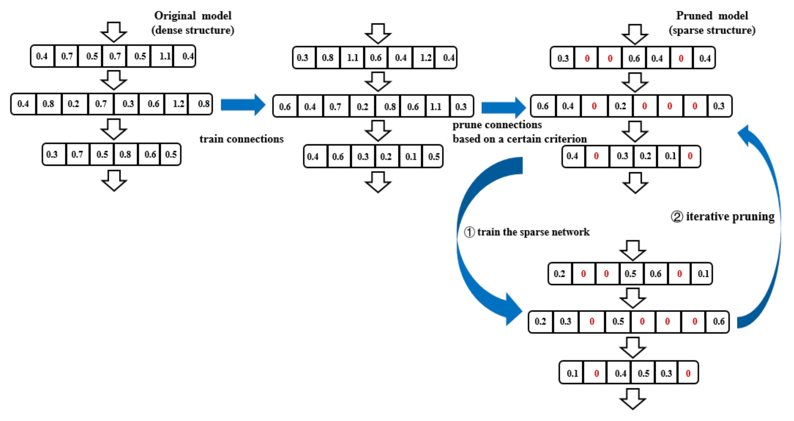
Specifically, whether it is the neuron (channel, filter) pruning or weight pruning of a dense network, the pruning process can be divided into one-shot pruning and iterative pruning. The former first evaluates the importance of connection parameters in the pre-trained model. After that, all unimportant parameters of a certain percentage are directly cut off (by calculated thresholds or other constraints) at once. On the contrary, the iterative pruning flow usually steps up from a low ratio to the targeted compression ratio gradually. Meanwhile, after the pruning operation, the network is usually fine tuned to compensate for lost accuracy, retraining the sparse network with unremoved parameters. The common iterative pruning procedure can be described as in Figure 7. Those zero values marked in red denote the discarded values.

The original untrained model with a dense structure is first trained to be converged, then iteratively pruning and training operations are applied for achieving the satisfactory performance at a given pruning rate. Therefore, pruning can learn useful connections, while storing the sparse network will help reduce computational burden and storage size with some specific storage formats.

Commonly, the selection for less important parameters to be removed usually rely on a certain criterion calculation, learning which connections are unimportant and then discarding them. Some studies suggested that the impact of parameter changes on the loss function should be evaluated. It is a relatively expensive, time consuming task to compute the loss after eliminating each parameter. The earlier work Optimal Brain Damage and Optimal Brain Surgeon proposed to calculate the Taylor expansion of the gradient of the optimization objective with respect to the weight parameters, which need to compute the Hessian matrices containing the second-order terms or its approximation [59,60]. Intuitively, the contribution of each connection in the entire network can be estimated by itself concerning magnitude and smaller numerical value together with a smaller contribution to the entire network performance. Hence, magnitude-based pruning (e.g., absolute values) is the more widely recognized and used method concerning the criteria for selecting unimportant elements to be removed.

3.2. Pruning Implementation

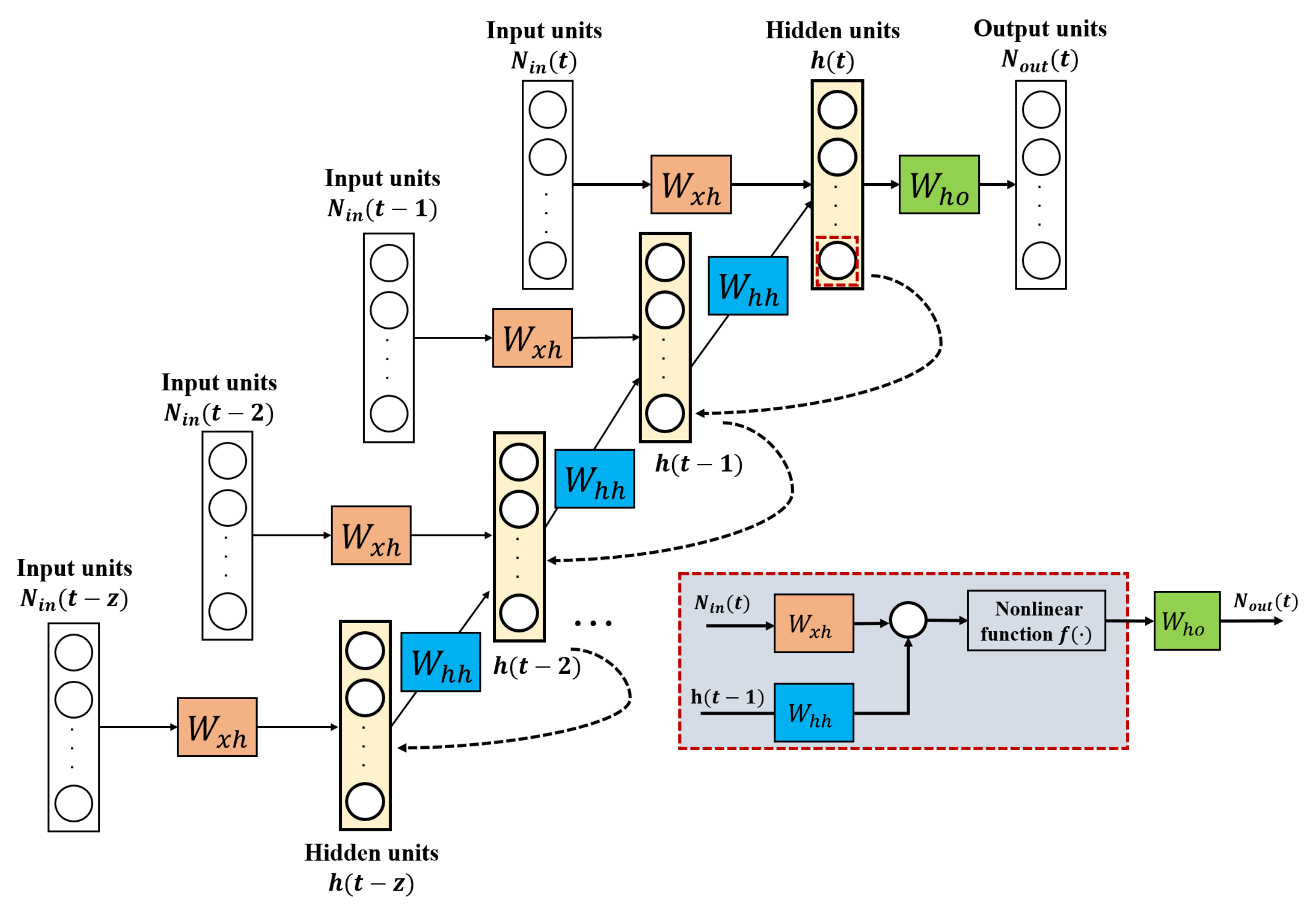
Our pruning procedure is combined with three binary mask matrices in different layers, expressed by $M^{\left(l\right)}\in {\{0,1\}}^{W^l}$, which are in the form of a binary mask, with the same size as the individual weight matrices W${}^{\left(l\right)}$ with l∈$\left[xh,hh,ho\right]$ in our RNN model. They will fix the less important parameters to be zero by $M^{\left(l\right)}$⊙$W^{\left(l\right)}$, where ⊙ denotes the element-wise product operation.

We use the symbol $W_{i,j}^{\left(l\right)}$, which denotes the parameters connecting the layer l with j units to the last layer $l-1$ with i units. The unimportant connections to be removed can be determined by ranking the magnitude-based values of the model; the threshold for discarding those lowest values is calculated for the given pruning rates. For each layer, every connection parameter after the mask operations is expressed as ${\hat{W}}_{i,j}^{\left(l\right)}$ and can be formulated as:

$${\hat{W}}_{i,j}^{\left(l\right)}=\left\{\begin{array}{cc}0,& if W_{i,j}^{\left(l\right)}<threshold\\ W_{i,j}^{\left(l\right)},& Otherwise\end{array}\right.$$

(12)

The detailed procedure of the weight pruning operation for our well-trained RNN-based temperature model is summarized as follows:

Step 1: From the pre-trained model, we extract the input and hidden layers containing weight connections $W^{\left(xh\right)}$ and $W^{\left(hh\right)}$ and put them together to rank these connections based on absolute magnitudes of them. Then the threshold of which values to be removed at the given pruning rate are obtained.

Step 2: Guided by the threshold, the mask vectors for the connection $W^{\left(xh\right)}$ and $W^{\left(hh\right)}$ are updated and the unimportant connections removed from the weight matrices are as in Equation (12), those preserved as 1 and pruned as 0. Then the extracted input–hidden layer performs the forward calculation with the pruned weight matrices and gets the hidden output ${\hat{y}}_h$.

Step 3: Calculate the least square loss ${\epsilon }_h$ between the model outputs of original $y_h$ and ${\hat{y}}_h$ with masked connections, as expressed in Equation (13), where ${∥·∥}_2$ represents the $l_2$-norm. Modify a standard calculation formulation as written in Equation (14), the network follows Equation (15) to do backpropagation (BP) computation with the masked weight vectors $W^{\left(xh\right)}$ and $W^{\left(hh\right)}$.

Step 4: The updated parameters are imported into the network for inferencing and fine tuning the preserved parameters until the network converges.

Step 5: After pruning the connections of input layer and hidden layer, trained parameters and mask vectors are preserved for the output layer pruning, the optimization problem of output layer backs to the objective function (5); the weights of output layer is removed by the threshold calculated at the pruning rate.

$${\epsilon }_h=\frac{1}{2N}{∥y_h-{\hat{y}}_h∥}_2^2$$

(13)

$$W_{i,j}^{\left(l\right)}:=W_{i,j}^{\left(l\right)}+\eta \frac{\partial \epsilon }{\partial W_{i,j}^{\left(l\right)}}$$

(14)

$$W_{i,j}^{\left(l\right)}:=W_{i,j}^{\left(l\right)}+\eta \frac{\partial {\epsilon }_h}{\partial (M_{i,j}^{\left(l\right)}\odot W_{i,j}^{\left(l\right)})}$$

(15)

Specifically, for an RNN model at time step t + 1, the derivation of gradients with respect to the input–hidden $W^{xh}$ and hidden–hidden $W^{hh}$ matrices needs to consider the time-step accumulation from t to 0, called backpropagation through time as introduced in Section; we use the chain rule to calculate them at time step t + 1, written as follows:

$$\frac{\partial \epsilon (t+1)}{\partial W_{xh}}=\sum _{k=1}^{t+1}\frac{\partial \epsilon (t+1)}{\partial h_{t+1}}\frac{\partial h_{t+1}}{\partial h_k}\frac{\partial h_t}{\partial W_{xh}}$$

(16)

$$\frac{\partial \epsilon (t+1)}{\partial W_{hh}}=\sum _{k=1}^{t+1}\frac{\partial \epsilon (t+1)}{\partial z_{t+1}}\frac{\partial z_{t+1}}{\partial h_{t+1}}\frac{\partial h_{t+1}}{\partial h_k}\frac{\partial h_t}{\partial W_{hh}}$$

(17)

3.3. Pruning Results

For various pre-trained ref-model based RNN temperature control models with different size of weight parameters, the same pruning operation is performed to reduce the randomness of results. We perform the same pruning process on the pre-trained networks based on our temperature control system, which consists of 40 hidden units and 120 hidden units, respectively. The weight size of the pre-trained RNN model is $W_{xh}$ of 40 by 3, $W_{hh}$ of 40 by 40 and $W_{ho}$ of 1 by 40; the total weight parameters are 1760. Another is $W_{xh}$ of 120 by 3, $W_{hh}$ of 120 by 120 and $W_{ho}$ of 1 by 120, the total weight parameters are 14,880. The sum of the squared error between the actual temperature output and the proposed ref-model output for the temperature variation (from 100 ${}^{\circ }$C–105 ${}^{\circ }$C within 10,000 s, containing 20,000 data points) after adding disturbance is calculated as baseline for a comparison between the performance of the pre-trained model and that of the pruned model. The cost values for the pre-trained temperature control models with 40 and 120 hidden units are 2276.8 and 2189.9, respectively. The other basis settings of our pre-trained temperature control models are as described in Section 2.1.3 above, including the ref-model based RNN model with the initial learning rate of 1.0 × 10${}^{-9}$ and the Adam optimizer is implemented for adjusting learnable parameters.

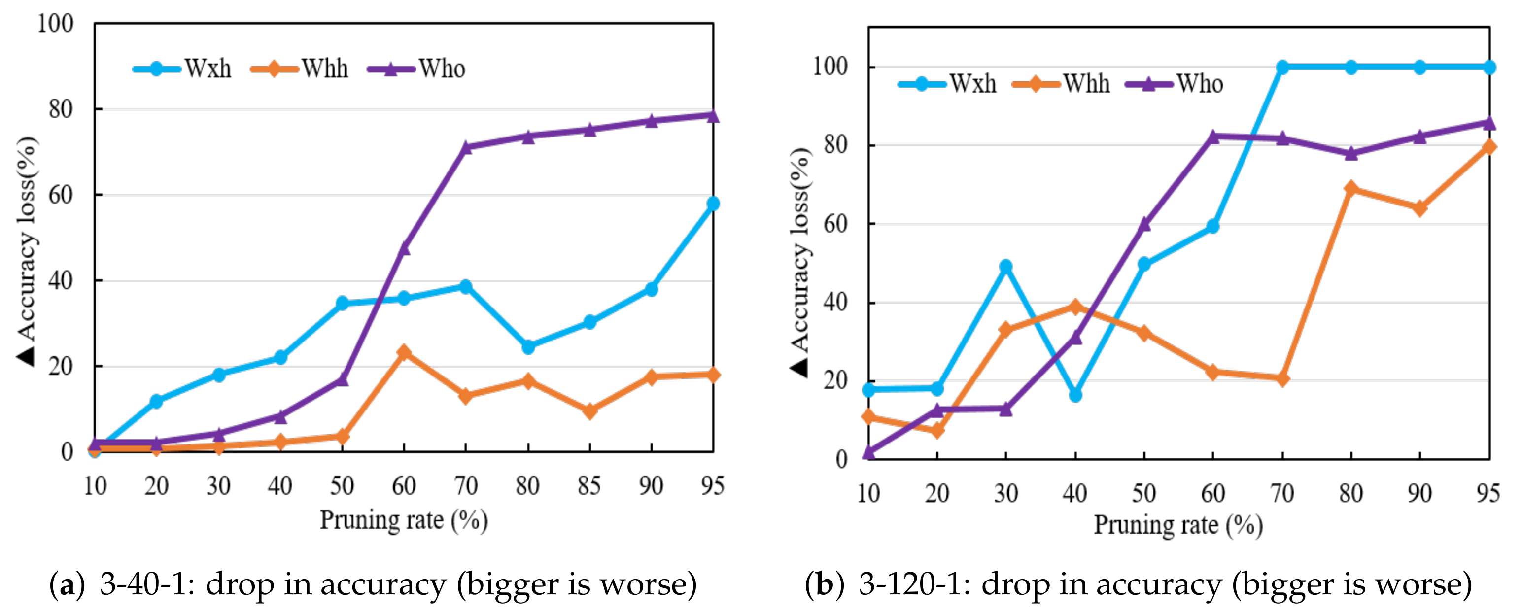
First of all, we do the experiments to observe how sensitive each weight matrix of different layers is to the increasing pruning rate. The weight matrices are independently pruned by the increasing pruning rates without retraining and the performances of the pruned model are compared with the initially pre-trained model. The accuracy differences after pruning each weight matrix are plotted in Figure 8.

The pruning rate indicates what proportion of the original parameters are put away, which set as zero. We do the same pruning operations in the pre-trained model with 40 hidden units and 120 hidden units separately. As Figure 8a shows, the performance losses after discarding each matrix parameters for given pruning rates are quite different; those of the input–hidden and hidden–hidden layer connections are relatively much higher than those of the hidden–hidden layer. In particular, when the pruning rate for $W_{ho}$ is greater than about 50% for the network with a 3-40-1 structure, it results in that the performance of the pruned model deteriorates drastically. In contrast, the performance loss of only pruning hidden–hidden layer weights $W_{hh}$ increased not so significantly as the pruning percentage is higher. Similarly, the performance loss of the network with a 3-120-1 structure after only removing $W_{xh}$ or $W_{ho}$ is much bigger than pruning the connections $W_{hh}$, as the pruning rate increases over 50%(Figure 8b). We can find the connections $W_{hh}$ account for a bigger proportion of all original connections than others initially having more redundancy to reduce. The original model which is more sensitive to the connection $W_{xh}$ and $W_{ho}$ decrease with the increasing pruning rates. At the same pruning rates, they result in much more performance loss of the system than $W_{hh}$. Therefore, in practice the hidden connection $W_{hh}$ can be more sharply trimmed than $W_{xh}$ and $W_{ho}$ while hurting the system performance less.

Then we do pruning experiments that directly remove the corresponding portion of the overall network parameters and retrain once. It is based on the global measured thresholds corresponding to the pruning rate, which puts all weight connections together and then asseses the importance of each parameter. The control performances of the pruned models with 10, 40 and 120 hidden neurons, respectively, deleting those redundant connections at different pruning rates and results are compared to the initial pre-trained model. Then the accuracies in percentage of the untrimmed model and thresholds with different pruning rates are shown in

Table 4. Comparison results of pruned model performance. With the increasing pruning rates, the percentage values represent the actual performances in proportion to the original pre-trained models (Acc (%)) and the threshold (Thre) is calculated at different rates in several models. Note that FLOPs represent the size of all pruned parameters.

Prune Rate (%)	Acc${}_{10}$ (%)	Thre${}_{10}$	FLOPs (KB)	Acc${}_{40}$ (%)	Thre${}_{40}$	FLOPs (KB)	Acc${}_{120}$ (%)	Thre${}_{120}$	FLOPs (KB)
10	99.02	0.0235	0.08	99.651	0.0108	1.03	89.276	0.0064	8.72
20	99.27	0.0414	0.17	99.583	0.0238	2.04	87.903	0.0133	17.44
30	97.29	0.0658	0.24	96.925	0.0366	3.09	84.758	0.0203	26.16
40	95.18	0.0899	0.33	95.281	0.0533	4.13	79.762	0.0275	34.88
50	90.35	0.1590	0.41	89.258	0.0631	5.16	89.240	0.0358	43.59
60	87.69	0.1855	0.49	74.702	0.0869	6.19	80.134	0.0452	52.31
70	88.28	0.2341	0.57	75.503	0.1108	7.22	79.668	0.0561	61.03
80	65.72	0.2891	0.66	69.558	0.1385	8.25	22.325	0.0627	69.75
90	32.20	0.4412	0.74	61.968	0.1932	9.28	21.387	0.0702	78.47

. In addition, the reduced memory overhead of the pruned model can be estimated by the ratio of reduced parameters of each weight matrix. Commonly, the pruned model size with the sparse structure can be saved in compressed sparse row format (CSR) to cut computational expense [61], the nonzero values can be stored by 32-bit floating-point, 4 bytes, while the row and column indices of each weight parameter are stored as 16-bit, 2 bytes. Hence, the pruned float point operations (FLOPs) with various pruning rates are approximately expressed in kilobyte and listed. The pruning thresholds of different models vary for the original weight distributions.

With the increasing pruning rates, although considering the overall network connections for removing parameter redundancy, it is obvious that the accuracy falls sharply when the pruning rate is over 60% in each model. Because the sparse models can not be directly adaptive to the initial parameters of the pre-trained networks, resulting in the remaining parameters not being able to keep the ideal performance. The damage to a network by deleting a large number of connections at once is not easily remedied. From previous studies [62,63], the compressed model obtained by the iterative pruning method is more compact and smaller, although its training cost is higher than that of the one-shot method, which prunes the connections to the desired percentage once. Discarding too many parameters at once can cause irreparable accuracy loss; therefore, it is more reasonable to gradually prune the network connections to the target sparsity.

Here, we adopt the iteratively layer-wise pruning approach to trim the pre-trained models, respectively. For example, if the given pruning rate is 80%, the connections are pruned to 20% based on the overall weights, and the preserved parameters are retrained until the network converges. After that, the model parameters are pruned to a higher pruning rate as the previous steps. The process is repeated until the model reaches the given sparsity. Note that retraining and pruning operations are performed alternately; those preserved connections can be retrained until the model reaches the desired performance concerning the increasing pruning rate. In addition, the learning rate of the pruned model also needs to be reduced relatively for adjusting the sparse network. Following the proposed layer-wise pruning method, we first compare the iteratively pruning and directly pruning (one-shot) experiment results of the original pre-trained model with 10 neurons; the pruning results from 10% to 90% are described in

Table 5. Comparison results of iterative pruning and one-shot pruning: Layer-wise pruning performance of the model with 10 hidden neurons. Acc${}_1^{one}$ (%) means the accuracy after removing the redundancy in W${}_{xh}$ and W${}_{hh}$ by one-shot pruning; then Acc${}_2^{one}$ (%) is after removing less important connections in W${}_{ho}$. Similarly, Acc${}^{iter}$ (%) denotes the results adopting the iterative method.

Pruned (%)	Acc${}_1^{\mathit{one}}$ (%)	Acc${}_2^{\mathit{one}}$ (%)	Acc${}_1^{\mathit{iter}}$ (%)	Acc${}_2^{\mathit{iter}}$ (%)	FLOPs (KB)
10	99.01	99.05	99.87	99.93	0.08
20	99.24	99.29	99.43	99.81	0.17
30	97.24	97.33	98.58	99.66	0.24
40	95.08	95.19	98.62	99.25	0.33
50	90.28	90.56	99.33	99.47	0.41
60	90.61	90.86	98.94	98.99	0.49
70	88.18	88.45	98.74	97.99	0.57
80	65.71	65.23	97.66	98.82	0.66
85	62.03	61.19	97.45	98.65	0.70
90	38.23	39.46	47.44	46.31	0.74

.

Comparing the accuracy of the model after discarding the connection W${}_{xh}$ and W${}_{hh}$ by directly pruning and retraining with that preforming iteratively pruning and retraining, from the results, the performances of the two methods are similar when the pruning rate is below 70%. With the pruning rate increasing, the model performance of the iterative pruning clearly outperforms that of directly pruning and retraining. Therefore, although the iterative pruning advantage is less obvious in a low pruning rate, it is useful to hold a higher accuracy in a high rate. For this RNN model in the temperature control system, the overall weight connections can be pruned to 15% without hurting the final performance. However, when the 95% percentage of overall network weights are discarded, the performance shifts down significantly. This demonstrates the limitation of the pruning rate to the pre-trained model; once too many connections are removed, the remaining model underfits the data.

Then, we perform nonlinear reconstruction error pruning and retrain iteratively on the pre-trained control models with 40 and 120 hidden neurons, respectively. The same learning rate of 1.0 × 10${}^{-10}$ with 50 retraining epochs after every pruning rate is used in our temperature control models; the pruned control models can converge and achieve relatively satisfactory results. The accuracy results of the layer-wise pruned models are shown in

Table 6. Iterative layer-wise pruning performance of the model with 40 hidden neurons. Acc${}_1^{iter}$ (%) is the accuracy after removing the redundancy in W${}_{xh}$ and W${}_{hh}$, and Acc${}_2^{iter}$ (%) is after removing less important connections in W${}_{ho}$. P${}_w$ (%) denotes the percentage of the removed weights over the entire network in different pruning rates.

Pruned (%)	Acc${}_1^{\mathit{iter}}$ (%)	Acc${}_2^{\mathit{iter}}$ (%)	FLOPs (KB)	P${}_{\mathit{Wxh}}$ (%)	P${}_{\mathit{Whh}}$ (%)	P${}_{\mathit{Who}}$ (%)
10	99.97	99.95	1.03	0.11	9.88	0
20	99.94	99.96	2.04	0.11	19.72	0.06
30	98.95	99.97	3.09	0.28	29.66	0.06
40	98.46	98.96	4.13	0.34	39.60	0.06
50	98.94	98.69	5.16	0.57	49.38	0.06
60	97.93	98.87	6.19	0.63	59.26	0.11
70	99.14	98.95	7.22	0.79	69.03	0.17
80	98.16	98.93	8.25	1.02	78.69	0.28
85	97.78	98.42	8.77	1.31	83.29	0.39
90	89.63	87.90	9.28	1.65	87.89	0.51

and

Table 7. Iterative layer-wise pruning performance of the model with 120 hidden neurons. P${}_w$ (%) denotes the percentage of the removed weights over the entire network in different pruning rates.

Pruned (%)	Acc${}_1^{\mathit{iter}}$ (%)	Acc${}_2^{\mathit{iter}}$ (%)	FLOPs (KB)	P${}_{\mathit{Wxh}}$ (%)	P${}_{\mathit{Whh}}$ (%)	P${}_{\mathit{Who}}$ (%)
10	97.89	98.22	8.72	0.01	9.98	0.01
20	98.24	99.33	17.44	0.05	19.93	0.02
30	89.12	99.18	26.16	0.05	29.93	0.02
40	93.45	97.44	34.88	0.08	39.89	0.03
50	88.87	98.88	43.59	0.11	49.85	0.04
60	92.56	98.54	52.31	0.14	59.82	0.04
70	95.76	97.33	61.03	0.17	69.78	0.05
80	97.12	96.56	69.75	0.19	79.75	0.06
85	91.12	90.62	74.11	0.21	84.72	0.07
90	67.12	65.13	78.47	0.25	89.66	0.09

.

From the results, we can also find when the pruning rate is below 80%, the performance decrease of the temperature control system is not obvious. The iterative layer-wise pruning results describe the accuracy after pruning each layer connection. However, when the pruning rate is too high such as from 80% to 90%, there is an obvious decrease in the performance of the temperature system. Too many parameters being removed makes it difficult for the models to fit the data. In terms of the percentage concerning weights that are removed, there are a lot of redundant parameters in the hidden layer. The pruning limitation of the pre-trained models with 40 and 120 hidden units is about 85% and 80%, respectively. The current sparse network models reduce a high percentage of hidden layer connections without damaging the system performance, thus effectively saving the plenty of storage space compared to the original pre-trained model. From the results, although we adopt the magnitude-based pruning method for deleting the parameters, the original model with large dimension may lose some important parameters as the pruning rate increases, which are actually related to the remaining parameters in the original model and have a great impact on the final performance of the system, and in practice the lost accuracy is hard to recover within limited epochs.

Finally, to verify the control performance of the pruned models with different hidden units by the layer-wise reconstruction error method, we list the final response characteristics of our temperature system with the disturbance signal under the same conditions of experiments. As

Table 8. Response characteristics comparison between the pruned models with various structures and the original pre-trained model. The overshoot value represents the maximum offset of the temperature variations in the rising process.

Mode	2% Settling Time [s]	Drop [${}^{\circ }$C]	Overshoot [${}^{\circ }$C]	Pruned [%]
Baseline	2815 (100%)	1.7 (100%)	0.7 (100%)	0
3-10-1	2847 (1.1%)	1.73 (1.8%)	0.71 (1.4%)	80
3-40-1	2918 (3.6%)	1.78 (4.7%)	0.71 (2.4%)	80
3-120-1	2944 (4.6%)	1.78 (4.7%)	0.73 (4.2%)	80

shows, the differences between the original pre-trained model and the trimmed model with 10 hidden units in 80% pruning rate are less than 2%. The settling time is 2847 s, which has a slight increase of 1.1%, and the fluctuation of drop and overshoot in temperature are 1.8% and 1.4% compared to the original pre-trained model, respectively. Similarly, the difference between the pruned model with 40 and 120 hidden units has a slight higher percentage deviation within about 5% in the same pruning rate of 80%. The pruned model can also obtain a similar control effect with the remaining parameters.

4. Discussion and Conclusions

In this paper, we first verified the effectiveness of the proposed RNN model based real-time temperature control method through experiments. The RNN model is combined with a pre-designed model that provides the desired temperature output; it can, in a timely manner, adjust the control signal by minimizing the error between the ref-model and the actual controlled objective outputs. Compared to the conventional IPD controller, the temperature responds more quickly and has a smoother transition from the initial to the steady-state of the target value. In addition, the disturbance response of our system is also verified from the obtained experimental results. The object temperature can still restore to the ideal state after receiving a disturbance signal, concerning which both dynamic and steady-state response are also superior to the traditional controller.

Then, the pre-trained RNN-based temperature control model is further compressed by the pruning technology. Based on the popular layer-wise neuron pruning strategy for the CNN models, we extend it to our RNN-based temperature control model, reconstructing the nonlinear error between the original model and the pruned model outputs in hidden layer, and then further pruning the output layer iteratively. From the results, this pruning method is useful and effective in removing the redundant connections of our RNN-based temperature control model, while ensuring the final performance in the high pruning rate. Meanwhile, the experiment results show that this method with iteration and retraining can obtain a higher accuracy than that directly removing and retraining with the increasing pruning rate.

In our further work, we plan to explore the pruning limitation of each weight matrix, to improve the selection of unimportant connections in the RNN model and make the pruning process of our temperature control model more effective. More importantly, how to combine with more effective methods like weight quantization for easier implementation in hardware needs more research.

References

1. Fehrenbacher, A.; Duffie, N.A.; Ferrier, N.J.; Pfefferkorn, F.E.; Zinn, M.R. Effects of tool—Workpiece interface temperature on weld quality and quality improvements through temperature control in friction stir welding. Int. J. Adv. Manuf. Technol. 2014, 71, 165–179. [Google Scholar] [CrossRef]
2. Lundén, J.; Vanhanen, V.; Myllymäki, T.; Laamanen, E.; Kotilainen, K.; Hemminki, K. Temperature control efficacy of retail refrigeration equipment. Food Control 2014, 45, 109–114. [Google Scholar] [CrossRef]
3. Song, J.L.; Cheng, W.L.; Xu, Z.M.; Yuan, S.; Liu, M.H. Study on PID temperature control performance of a novel PTC material with room temperature Curie point. Int. J. Heat Mass Transf. 2016, 95, 1038–1046. [Google Scholar] [CrossRef] [Green Version]
4. Oldewurtel, F.; Parisio, A.; Jones, C.N.; Gyalistras, D.; Gwerder, M.; Stauch, V.; Morari, M. Use of model predictive control and weather forecasts for energy efficient building climate control. Energy Build. 2012, 45, 15–27. [Google Scholar] [CrossRef] [Green Version]
5. Shein, W.W.; Tan, Y.; Lim, A.O. PID Controller for Temperature Control with Multiple Actuators in Cyber-Physical Home System. In Proceedings of the IEEE 15th International Conference on Network-Based Information Systems, Melbourne, VIC, Australia, 26–28 September 2012; pp. 423–428. [Google Scholar]
6. Forbes, M.G.; Patwardhan, R.S.; Hamadah, H.; Gopaluni, R.B. Model predictive control in industry: Challenges and opportunities. IFAC-PapersOnLine 2015, 48, 531–538. [Google Scholar] [CrossRef]
7. Ma, Y.; Guo, G. (Eds.) Support Vector Machines Applications; Springer: New York, NY, USA, 2014. [Google Scholar]
8. Singh, S.; Hussain, S.; Bazaz, M.A. Short term load forecasting using artificial neural network. In Proceedings of the IEEE 2017 4th International Conference on Image Information Processing (ICIIP), Shimla, India, 21–23 December 2017; pp. 1–5. [Google Scholar]
9. Chauhan, N.K.; Singh, K. A review on conventional machine learning vs deep learning. In Proceedings of the IEEE 2018 International Conference on Computing, Power and Communication Technologies (GUCON), Greater Noida, India, 28–29 September 2018; pp. 347–352. [Google Scholar]
10. Lipton, Z.C.; Berkowitz, J.; Elkan, C. A critical review of recurrent neural networks for sequence learning. arXiv 2015, arXiv:1506.00019. [Google Scholar]
11. Pascanu, R.; Gulcehre, C.; Cho, K.; Bengio, Y. How to construct deep recurrent neural networks. arXiv 2013, arXiv:1312.6026. [Google Scholar]
12. Jin, L.; Li, S.; Hu, B. RNN models for dynamic matrix inversion: A control-theoretical perspective. IEEE Trans. Ind. Inform. 2017, 14, 189–199. [Google Scholar] [CrossRef]
13. Samarawickrama, A.J.P.; Fernando, T.G.I. A recurrent neural network approach in predicting daily stock prices an application to the Sri Lankan stock market. In Proceedings of the IEEE International Conference on Industrial and Information Systems (ICIIS), Peradeniya, Sri Lanka, 15–16 December 2017; pp. 1–6. [Google Scholar]
14. Raj, J.S.; Ananthi, J.V. Recurrent neural networks and nonlinear prediction in support vector machines. J. Soft Comput. Paradig. (JSCP) 2019, 1, 33–40. [Google Scholar] [CrossRef]
15. Nivison, S.A.; Khargonekar, P.P. Development of a robust deep recurrent neural network controller for flight applications. In Proceedings of the American Control Conference (ACC), Seattle, WA, USA, 24–26 May 2017; pp. 5336–5342. [Google Scholar]
16. De Mulder, W.; Bethard, S.; Moens, M.F. A survey on the application of recurrent neural networks to statistical language modeling. Comput. Speech Lang. 2015, 30, 61–98. [Google Scholar] [CrossRef] [Green Version]
17. Liu, J.; Tripathi, S.; Kurup, U.; Shah, M. Pruning algorithms to accelerate convolutional neural networks for edge applications: A survey. arXiv 2020, arXiv:2005.04275. [Google Scholar]
18. Liang, T.; Glossner, J.; Wang, L.; Shi, S.; Zhang, X. Pruning and quantization for deep neural network acceleration: A survey. Neurocomputing 2021, 461, 370–403. [Google Scholar] [CrossRef]
19. Guo, Y.; Yao, A.; Chen, Y. Dynamic network surgery for efficient dnns. arXiv 2016, arXiv:1608.04493. [Google Scholar]
20. Lazarevic, A.; Obradovic, Z. Effective pruning of neural network classifier ensembles. In Proceedings of the International Joint Conference on Neural Networks Proceedings (Cat. No.01CH37222), Washington, DC, USA, 15–19 July 2001; pp. 796–801. [Google Scholar]
21. Sze, V.; Chen, Y.H.; Yang, T.J.; Emer, J.S. Efficient processing of deep neural networks: A tutorial and survey. Proc. IEEE 2017, 105, 2295–2329. [Google Scholar] [CrossRef] [Green Version]
22. Zhao, C.; Ni, B.; Zhang, J.; Zhao, Q.; Zhang, W.; Tian, Q. Variational convolutional neural network pruning. In Proceedings of the IEEE/CVF Conference on Computer Vision and Pattern Recognition, Long Beach, CA, USA, 15–20 June 2019; pp. 2780–2789. [Google Scholar]
23. Han, S.; Mao, H.; Dally, W.J. Deep compression: Compressing deep neural networks with pruning, trained quantization and huffman coding. arXiv 2015, arXiv:1510.00149. [Google Scholar]
24. Molchanov, P.; Tyree, S.; Karras, T.; Aila, T.; Kautz, J. Pruning convolutional neural networks for resource efficient inference. arXiv 2016, arXiv:1611.06440. [Google Scholar]
25. Liu, Z.; Sun, M.; Zhou, T.; Huang, G.; Darrell, T. Rethinking the value of network pruning. arXiv 2018, arXiv:1810.05270. [Google Scholar]
26. Han, S.; Pool, J.; Tran, J.; Dally, W.J. Learning both weights and connections for efficient neural networks. arXiv 2015, arXiv:1506.02626. [Google Scholar]
27. Anwar, S.; Hwang, K.; Sung, W. Structured pruning of deep convolutional neural networks. ACM J. Emerg. Technol. Comput. Syst. (JETC) 2017, 13, 1–18. [Google Scholar] [CrossRef] [Green Version]
28. Lemaire, C.; Achkar, A.; Jodoin, P.M. Structured pruning of neural networks with budget-aware regularization. In Proceedings of the IEEE/CVF Conference on Computer Vision and Pattern Recognition, Long Beach, CA, USA, 15–20 June 2019; pp. 9108–9116. [Google Scholar]
29. Wen, W.; Wu, C.; Wang, Y.; Chen, Y.; Li, H. Learning structured sparsity in deep neural networks. Adv. Neural Inf. Process. Syst. 2016, 30, 2074–2082. [Google Scholar]
30. Srinivas, S.; Babu, R.V. Data-free parameter pruning for deep neural networks. arXiv 2015, arXiv:1507.06149. [Google Scholar]
31. Zhuang, Z.; Tan, M.; Zhuang, B.; Liu, J.; Guo, Y. Discrimination-aware channel pruning for deep neural networks. arXiv 2018, arXiv:1810.11809. [Google Scholar]
32. Huang, G.; Liu, S.; Van der Maaten, L.; Weinberger, K.Q. Condensenet: An efficient densenet using learned group convolutions. In Proceedings of the IEEE Conference on Computer Vision and Pattern Recognition, Salt Lake City, UT, USA, 18–23 June 2018; pp. 2752–2761. [Google Scholar]
33. He, Y.; Zhang, X.; Sun, J. Channel pruning for accelerating very deep neural networks. In Proceedings of the IEEE International Conference on Computer Vision, Venice, Italy, 22–29 October 2017; pp. 1398–1406. [Google Scholar]
34. Blalock, D.; Ortiz, J.J.G.; Frankle, J.; Guttag, J. What is the state of neural network pruning? arXiv 2020, arXiv:2003.03033. [Google Scholar]
35. He, Y.; Liu, P.; Wang, Z.; Hu, Z.; Yang, Y. Filter pruning via geometric median for deep convolutional neural networks acceleration. In Proceedings of the IEEE/CVF Conference on Computer Vision and Pattern Recognition (CVPR), Long Beach, CA, USA, 15–20 June 2019; pp. 4340–4349. [Google Scholar]
36. Gale, T.; Zaharia, M.; Young, C.; Elsen, E. Sparse GPU kernels for deep learning. In Proceedings of the International Conference for High Performance Computing, Networking, Storage and Analysis, Atlanta, GA, USA, 9–19 November 2020; pp. 1–14. [Google Scholar]
37. Wang, Z. Sparsert: Accelerating unstructured sparsity on gpus for deep learning inference. arXiv 2020, arXiv:2008.11849. [Google Scholar]
38. Ma, X.; Guo, F.M.; Niu, W.; Lin, X.; Tang, J. Pconv: The missing but desirable sparsity in dnn weight pruning for real-time execution on mobile devices. In Proceedings of the AAAI Conference on Artificial Intelligence, New York, NY, USA, 7–12 February 2020; pp. 5117–5124. [Google Scholar]
39. Liu, Y.; Xu, S.; Kobori, S.; Hashimoto, S.; Kawaguchi, T. Time-Delay Temperature Control System Design based on Recurrent Neural Network. In Proceedings of the 4th IEEE International Conference on Industrial Cyber-Physical Systems (ICPS), Victoria, BC, Canada, 10–12 May 2021; pp. 820–825. [Google Scholar]
40. Dong, X.; Chen, S.; Pan, S.J. Learning to prune deep neural networks via layer-wise optimal brain surgeon. arXiv 2017, arXiv:1705.07565. [Google Scholar]
41. Chen, S.; Zhao, Q. Shallowing deep networks: Layer-wise pruning based on feature representations. IEEE Trans. Pattern Anal. Mach. Intell. 2018, 41, 3048–3056. [Google Scholar] [CrossRef]
42. Jiang, C.; Li, G.; Qian, C.; Tang, K. Efficient DNN Neuron Pruning by Minimizing Layer-wise Nonlinear Reconstruction Error. In Proceedings of the IJCAI, Stockholm, Sweden, 13–19 July 2018; p. 2. [Google Scholar]
43. Kaya, I. I-PD controller design for integrating time delay processes based on optimum analytical formulas. IFAC-PapersOnLine 2018, 51, 575–580. [Google Scholar] [CrossRef]
44. Das, S.; Chakraborty, A.; Ray, J.K.; Bhattacharjee, S.; Neogi, B. Study on different tuning approach with incorporation of simulation aspect for ZN (Ziegler-Nichols) rules. Int. J. Sci. Res. Publ. 2012, 2, 1–5. [Google Scholar]
45. Nakanishi, J.; Schaal, S. Feedback error learning and nonlinear adaptive control. Neural Netw. 2004, 17, 1453–1465. [Google Scholar] [CrossRef] [PubMed] [Green Version]
46. Rudin, W. Principles of Mathematical Analysis; McGraw-Hill: New York, NY, USA, 1964; Volume 3. [Google Scholar]
47. Xu, S.; Hashimoto, S.; Jiang, Y.; Izaki, K.; Kihara, T. A Reference-Model-Based Artificial Neural Network Approach for a Temperature Control System. Processes 2020, 8, 50. [Google Scholar] [CrossRef] [Green Version]
48. Ashar, N.D.B.K.; Yusoff, Z.M.; Ismail, N.; Hairuddin, M.A. ARX model identification for the real-time temperature process with Matlab-arduino implementation. ICIC Express Lett. 2020, 14, 103–111. [Google Scholar]
49. He, K.; Zhang, X.; Ren, S.; Sun, J. Delving Deep into Rectifiers: Surpassing Human-Level Performance on ImageNet Classification. In Proceedings of the 2015 IEEE International Conference on Computer Vision, Washington, DC, USA, 7–13 December 2015; pp. 1026–1034. [Google Scholar]
50. Ruder, S. An overview of gradient descent optimization algorithms. arXiv 2016, arXiv:1609.04747. [Google Scholar]
51. Seo, S.; Kim, J. Efficient weights quantization of convolutional neural networks using kernel density estimation based non-uniform quantizer. Appl. Sci. 2019, 9, 2559. [Google Scholar] [CrossRef] [Green Version]
52. Leng, C.; Dou, Z.; Li, H.; Zhu, S.; Jin, R. Extremely low bit neural network: Squeeze the last bit out with admm. In Proceedings of the Thirty-Second AAAI Conference on Artificial Intelligence, New Orleans, LA, USA, 2–7 February 2018. [Google Scholar]
53. Zhu, C.; Han, S.; Mao, H.; Dally, W.J. Trained ternary quantization. arXiv 2016, arXiv:1612.01064. [Google Scholar]
54. Ye, S.; Zhang, T.; Zhang, K.; Li, J.; Xie, J.; Liang, Y.; Wang, Y. A unified framework of dnn weight pruning and weight clustering/quantization using admm. arXiv 2018, arXiv:1811.01907. [Google Scholar]
55. Li, H.; Kadav, A.; Durdanovic, I.; Samet, H.; Graf, H.P. Pruning filters for efficient convnets. arXiv 2016, arXiv:1608.08710. [Google Scholar]
56. Hinton, G.E.; Srivastava, N.; Krizhevsky, A.; Sutskever, I.; Salakhutdinov, R.R. Improving neural networks by preventing co-adaptation of feature detectors. arXiv 2012, arXiv:1207.0580. [Google Scholar]
57. Wan, L.; Zeiler, M.; Zhang, S.; Le Cun, Y.; Fergus, R. Regularization of neural networks using dropconnect. In Proceedings of the International Conference on Machine Learning, Atlanta, GA, USA, 16–21 June 2013; pp. 1058–1066. [Google Scholar]
58. Luo, J.H.; Wu, J.; Lin, W. Thinet: A filter level pruning method for deep neural network compression. In Proceedings of the IEEE International Conference on Computer Vision, Venice, Italy, 22–29 October 2017; pp. 5058–5066. [Google Scholar]
59. Hassibi, B.; Stork, D.G. Second Order Derivatives for Network Pruning: Optimal Brain Surgeon; Morgan Kaufmann: San Mateo, CA, USA, 1993; pp. 164–171. [Google Scholar]
60. Martens, J.; Sutskever, I.; Swersky, K. Estimating the Hessian by back-propagating curvature. arXiv 2012, arXiv:1206.6464. [Google Scholar]
61. Koza, Z.; Matyka, M.; Szkoda, S.; Mirosław, Ł. Compressed multirow storage format for sparse matrices on graphics processing units. SIAM J. Sci. Comput. 2014, 36, C219–C239. [Google Scholar] [CrossRef] [Green Version]
62. Frankle, J.; Carbin, M. The lottery ticket hypothesis: Finding sparse, trainable neural networks. arXiv 2018, arXiv:1803.03635. [Google Scholar]
63. Tan, C.M.J.; Motani, M. DropNet: Reducing Neural Network Complexity via Iterative Pruning. In Proceedings of the 37th International Conference on Machine Learning, Vienna, Austria, 12–18 July 2020; pp. 9356–9366. [Google Scholar]
Figure 1. Proposed RNN-model based temperature control system.
Processes 10 00044 g001
Figure 2. Feedforward and backpropagation for RNN controller.
Processes 10 00044 g002
Figure 3. Experimental setup of the temperature control system.
Processes 10 00044 g003
Figure 4. Imported input signal and obtained output data for the thermal process, involving the temperature going up and down from the room temperature.
Processes 10 00044 g004
Figure 5. Dynamic responses of the control process with IPD and RNN controller, respectively. (a) The whole response for temperature goes from room temperature to a setpoint and then repeatedly responds to the rising and falling step signals. (b) The temperature change in positive and negative directions over a full cycle.
Processes 10 00044 g005
Figure 6. Dynamic response with a disturbance. (a) The whole disturbance response from temperature to setpoint and periodic changes in different directions. (b) The local magnified responses after adding disturbance signal.
Processes 10 00044 g006
Figure 7. Flow chart of the iterative pruning procedure.
Processes 10 00044 g007
Figure 8. Performance loss after pruning each layer connection in the pre-trained models with different hidden units; a smaller loss represents less sensitivity to the same pruning ratio.
Processes 10 00044 g008