Abstract
As obtained geofluids from enhanced geothermal systems usually have lower temperatures and contain chemicals and impurities, a novel power cycle (NPC) with a unit capacity of several hundred kilowatts has been configured and developed in this study, with particular reference to the geofluid temperature (heat source) ranging from 110 °C to 170 °C. Using a suitable CO2-based mixture working fluid, a transcritical power cycle was developed. The novelty of the developed power cycle lies in the fact that an increasing-pressure endothermic process was realized in a few-hundred-meters-long downhole heat exchanger (DHE) by making use of gravitational potential energy, which increases the working fluid’s pressure and temperature at the turbine inlet and, hence, increases the cycle’s power output. The increasing-pressure endothermic process in the DHE has a better match with the temperature change of the heat source (geofluid), as does the exothermic process in the condenser with the temperature change of the sink (cooling water), which reduces the heat transfer irreversibility and improves the cycle efficiency. Power cycle performance has been analyzed in terms of the effects of mass fraction of the mixture working fluids, the working fluid’s flowrate and its DHE inlet pressure, geofluid flowrate, and the length of the DHE. Results show that, for a given geofluid’s temperature and mass flowrate, the cycle’s net power output is a strong function of the working-fluid’s flowrate, as well as of its DHE inlet pressure. Too high or too low of a DHE inlet pressure results in a lower power output. When geofluid temperature is 130 °C, the optimum DHE inlet pressure is found to be 11 MPa, corresponding to an optimum working-fluid flowrate of 6.5 kg/s. The longer the DHE, the greater the corresponding working-fluid flowrate and the higher the net power output. For geofluid temperature ranging from 110 °C to 170 °C, the developed NPC has a better thermodynamic performance than the conventional ORC. The advantage of using the developed NPC becomes obvious when geofluid temperature is low. The maximum net power output difference between the NPC and the ORC happens when the geofluid temperature is 130 °C and NPC’s working fluid mass fraction (R32/CO2) is 0.5/0.5.
1. Introduction
In recent years, utilization of enhanced geothermal system (EGS) geothermal energy has attracted increasing attention. As most obtained geofluids from the EGS geothermal resources usually have lower temperatures and contain chemicals and impurities, binary cycle geothermal power generation technologies associated with ORC (organic Rankine cycle) or TRC (transcritical Rankine cycle) were usually proposed [1,2,3].
Binary ORC is a relatively common technology using medium or low temperature geothermal resource for power generation [4,5]. Compared with the subcritical ORC, TRC has an advantage in reducing the heat transfer irreversibility when the supercritical working fluid is gaining heat from the heat source, because the temperature of the working fluid is not constant during this heating process, which has a better match with the heat source temperature change [6]. Research on TRC with CO2 as working fluid was carried out by Zhang et al. [7]; they studied a solar thermal power generation cycle using CO2 as working fluid and obtained the thermal efficiency of power generation cycles and COP (coefficients of performance) [8] during summer and winter in Japan through experiments. Chan et al. [9] compared the performance of a carbon dioxide-based transcritical power cycle and an ORC using R123 as working fluid in industrial waste heat recovery and found that TRC had a higher power output than ORC.
CO2 has good mobility and excellent heat transfer performance, so it has been considered to be a suitable geothermal exploitation fluid or a working fluid for power cycles. Compared with water, CO2 has higher density sensitivity to temperature; using CO2 as geothermal exploitation fluid will provide a buoyancy-driven thermosiphon phenomenon [10] and hence reduce the power consumption of the circulation pump. Sun et al. [11] established a single-well geothermal model that used CO2 as a working fluid. They asserted that, compared with water, CO2 had a reduced heat mining capacity; however, it could obtain higher outlet pressure and temperature and could reduce the required pump power. Adams et al. [12] compared four CPG (CO2 plume geothermal) systems and two brine-based geothermal systems and found that the CPG direct geothermal system obtained the highest net power output. Although the use of CO2 as a TRC working fluid increases the parasitic losses, CO2 TRC still gets a higher net power output because CO2 has a better thermodynamic performance than the organic working fluid R245a. Amaya et al. proposed a different geothermal system [13]. They put a 330 m-long concentric tube as a downhole heat exchanger into the geothermal production well with upward flowing geofluid. CO2 was used as working fluid to absorb the heat from the geofluid through the concentric tube, and then directly entered a turbine for power generation. In this way, the problem of non-condensable gases (NCGs) in the geofluid was avoided, and a higher outlet temperature of working fluid in the downhole heat exchanger was obtained. Since they only used pure CO2 as a working fluid without using a pump in their experiment, the CO2 flowrate driven by the thermosiphon effect was relatively small; hence, the heat obtained from the geofluid was constrained by the CO2 flowrate. In their system, a supercritical CO2 Brayton cycle was used for power generation, with the turbine outlet pressure of CO2 being above its critical pressure.
Because the critical temperature of CO2 is low (31.2 °C), using pure CO2 as a working fluid for TRC will have a condensation problem. In most cases, the cooling-water temperature is close to, or even higher than, the critical temperature of CO2; hence, it is impossible to condense the exhaust vapor from the turbine. In this case, the cooling process cannot undergo a phase change unless under the supercritical condition, as happened in the CO2 Brayton cycle. Some recent studies showed that mixing another organic fluid that has a higher critical temperature with CO2 could solve this problem [14]. The CO2-based mixture working fluid allowed us to still use a conventional “condenser” (with phase change), instead of using “cooler” (with no phase change). Due to the temperature glide of the mixtures in the two-phase region, the temperature profile of the heat dissipation process in the condenser can be better matched with the cooling water and a less irreversible loss can be achieved. Dai et al. [15] used seven kinds of CO2-based mixtures as working fluids of a trans-critical Rankine cycle and analyzed the thermal efficiency and power output of the cycle; their results showed that power cycles using these mixture working fluids had higher thermal efficiencies and lower working-pressures compared with those when pure CO2 was used as a working fluid. Wu et al. [16] selected six CO2-based mixture working fluids as the working fluids of a geothermal power generation cycle and analyzed their thermal efficiency and economic performance. Their calculation result indicated that R161/CO2 had the highest thermal efficiency and economic performance and that the CPP (cost per net power) of the mixture was lower than that of CO2.
This study was inspired by the work carried out by Amaya et al. [13]. The aim of this study was to develop a power cycle (with a unit capacity of several hundred kilowatts) for enhanced geothermal systems supplying geofluids, with particular reference to the geofluid temperature (heat source) ranging from 120 °C to 170 °C. Different from the working fluid (pure CO2) and the power cycle (Brayton cycle) that Amaya et al. adopted, in this study, CO2-based mixture working fluids were investigated and a different power cycle was configured, which had the following characteristics:
- (1)
- The critical point of each CO2-based mixture working fluid investigated in this study is higher than that of the pure CO2; hence, a condensing process with phase change could be realized. As a result, a conventional condenser could be used, without being restricted to the use of costly large-area coolers, as in a Brayton cycle. Thus, it was thermodynamically possible to realize a transcritical power cycle with a higher thermal efficiency.
- (2)
- An increasing-pressure endothermic process (instead of an isobarically endothermic process) could be realized in a few-hundred-meters-long downhole heat exchanger (DHE) by making use of gravitational potential energy [17]. This resulted in an increase of the cycle’s heat gain. In addition, the CO2-based mixture working fluid used in this proposed power cycle had a obvious buoyancy-driven thermosiphon effect; hence, the working-fluid’s DHE outlet pressure (i.e., the working-fluid’s turbine inlet pressure) could be increased. As a result, the cycle’s power output was increased.
- (3)
- In the downhole heat exchanger (DHE), the working fluid absorbed heat from the geofluid with a higher temperature at depth; thus, a higher working-fluid’s DHE outlet temperature (i.e., a higher working-fluid’s turbine inlet temperature) could be obtained, which would also benefit the cycle’s power generation.
In this theoretical study, the proposed power cycle has been described in detail and its thermodynamic performance has been investigated by analyzing the influences of important parameters on the system. The investigated parameters included: mass fraction of the mixture working fluids, working fluid DHE inlet pressure and flowrate, geofluid flowrate, and length of the DHE. Different CO2-based mixture working fluids have been analyzed and their performances have been discussed, as well. In addition, thermodynamic performance (in terms of the net power output) has been compared between the proposed power cycle and the conventional organic Rankine cycle (ORC).
2. System Description
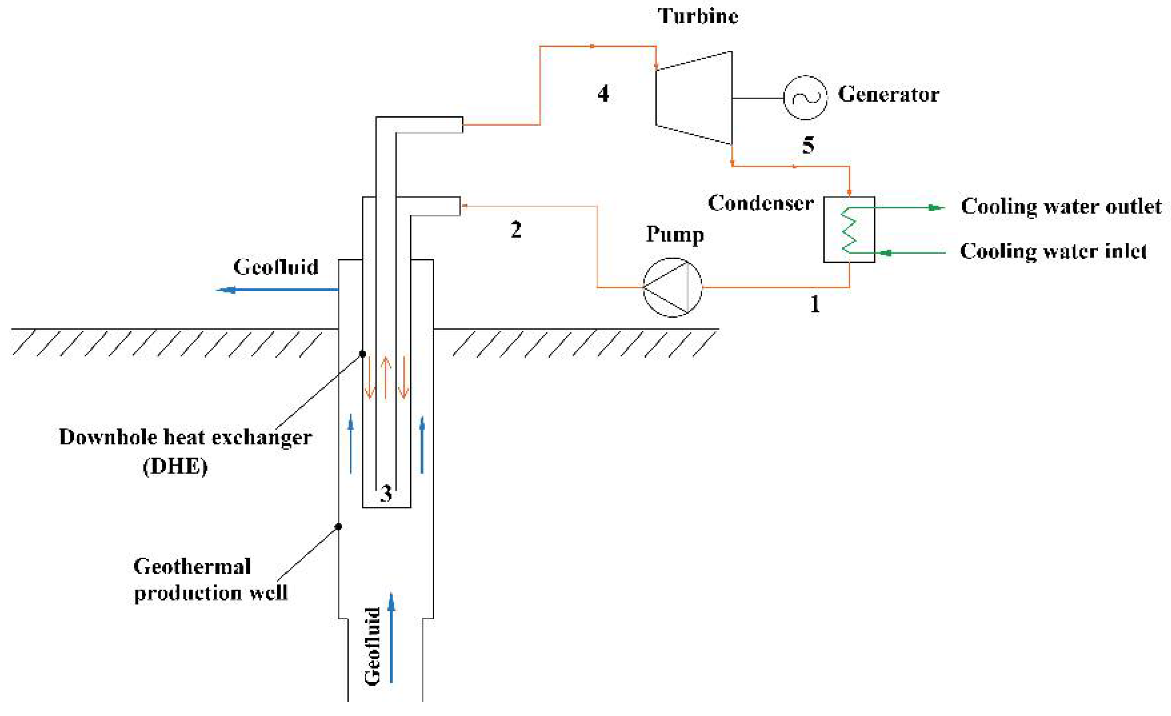
The schematic diagram of the geothermal power generation system investigated in this study is shown in Figure 1. Since enhanced geothermal systems can supply artesian geofluid in production wells, as reported by Hogarth and Bour (2015) [18], and Hogarth and Holl (2017) [19], it is assumed that the upward geofluid flow in the production well is artesian. The temperature-entropy (T-s) diagram of the power cycle corresponding to the system in Figure 1 is shown in Figure 2.
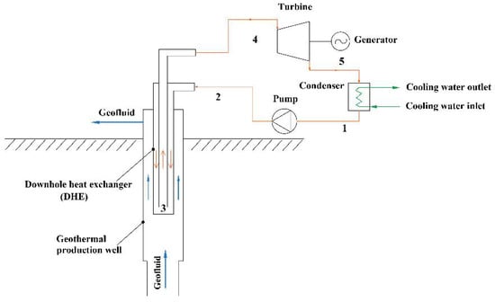
Figure 1.
Schematic diagram of the investigated geothermal power generation system.
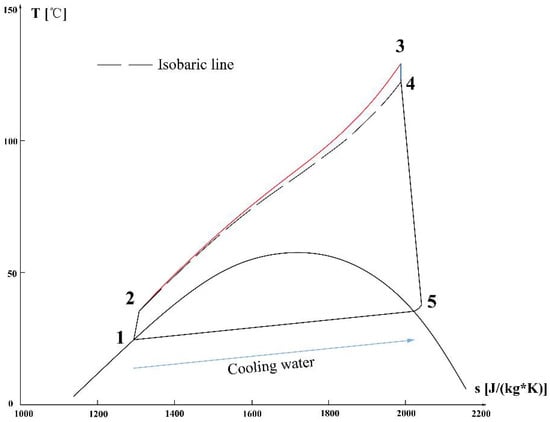
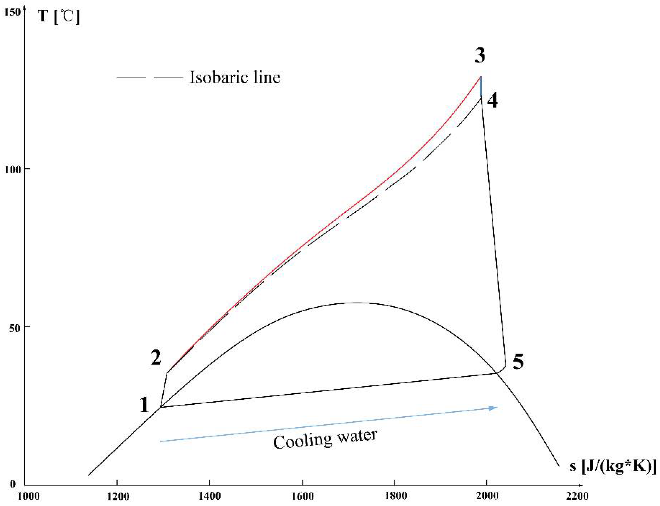
Figure 2.
Temperature-entropy (T-s) diagram of the power cycle corresponding to the power generation system shown in Figure 1 (geofluid temperature = 130 °C).
As can be seen in Figure 1, a coaxial double-pipe downhole heat exchanger is placed in a geothermal production well and forms a closed loop consisting of the turbine, condenser, and pump on the surface. The condensed working fluid (state 1) enters the pump and is pressurized into a supercritical condition (state 2) and is then injected into the downhole heat exchanger, forming a downward annulus flow that extracts heat from the upward flowing geofluid outside the heat exchanger, corresponding to the heat transfer process 2–3, as shown in the red line in Figure 2. The working fluid then moves into the inner pipe at the bottom of the downhole heat exchanger and flows upwards from the bottom (state 3) to the top (state 4), corresponding to the blue line (3–4) in Figure 2. The heated working fluid enters the turbine to generate shaft work (process 4–5) once it leaves the heat exchanger on the top. The exhaust (working fluid) of the turbine (state 5) is condensed in the condenser until it is in a saturated liquid state (state 1); then, another cycle starts.
When the working fluid flows downwards in the annulus, it forms a counter-flow with the geothermal water in the production well. This enables the working fluid to exchange heat with the deeper geothermal water at a higher temperature, resulting in a higher turbine inlet temperature and, hence, a higher power generation.
One unique feature of this power cycle lies in its increasing-pressure endothermic process, process 2–3 (the red line in Figure 2), which is determined based on the heat transfer model shown in Section 2 of this study. This increasing-pressure endothermic process can only be realized by taking advantage of the gravitational potential energy in a large-scale and closed-loop downhole heat exchanger. The dashed black line just below the red line in Figure 2 is a constant-pressure endothermic process (2–4) that occurs when the heat transfer between the geofluid and working fluid is made on the ground, as is commonly used in conventional ORC geothermal power stations. Simulation shows that the heat obtained by the mixture working fluid from process 2–3 is greater than that from process 2–4.
Since the mixture working fluid absorbs heat through the DHE at a few hundred-meter depth in the well and can get higher temperature, and since the buoyancy-driven thermosiphon effect in the DHE can boost the working-fluid’s DHE outlet pressure, the working-fluid’s temperature and pressure at the turbine inlet can be increased. As a result, the cycle’s power output becomes greater.
It is worth pointing out that the endothermic process under supercritical condition not only has a better match with the temperature change of the heat source (geofluid), but the exothermic process in condenser (5-1), which is a temperature-drop process, also has a better match with the temperature change of the cooling water. Both of them can reduce the heat transfer irreversibility and, hence, can improve the power cycle performance.
As mentioned earlier, CO2-based mixture working fluids have been investigated in this study. In the selection of working fluids, the following aspects have been considered: thermal properties, stability, toxicity, flammability, environmental friendliness, and price. The physical, safety and environmental data for some relevant refrigerants are shown in Table 1 [20]. The temperature glide characteristic of a mixture is an essential criterion in the selection. However, once the temperature glide exceeds a certain level, a high concentration shift and fractionation of the mixture components can appear [21]. In consideration of these factors, the following combinations were selected: CO2/R32, CO2/R1270, CO2/R161, CO2/R1234yf, CO2/R134a, CO2/R152a, and CO2/R1234ze. All the thermodynamic and transport properties of the mixtures have been calculated using REFPOP 9.0. The accuracy of each calculated property basically depends on the binary interaction parameter that is fitted by experimental data. According to Bell and Lemmon [22], the error can be less than 5% in the bubble point.

Table 1.
Physical, safety and environmental data of the refrigerants investigated.
3. Model Development
The power cycle model corresponding to the system described in Section 1 was developed. The mixture working fluid underwent the following major thermodynamic processes: expansion process in the turbine generating shaft work; non-isothermal condensation process in the condenser; pressurization process in the injection pump; and heat gaining process in the coaxial double-pipe downhole heat exchanger. The parameters used in the simulation can be found in Table 2. The condensation pressure is determined by the temperature of the cooling water and the pinch point method [9,23,24]. Because of the temperature glide of the mixtures during the condensation process, the problem of pinch points can be alleviated [25] and the utilization efficiency can be improved [26]. It is worth mentioning that the values of pump and turbine internal efficiencies used in this study are less than those adopted by previous theoretical studies [27,28,29,30], where the range of turbine efficiencies used is from 82% to 93%, and the range of compressor efficiencies used is from 81% to 93%.
Table 2.
Parameters used in the simulation.
As the coaxial double-pipe downhole heat exchanger and the geothermal production well are concentric, the 3-dimensional heat transfer model has been simplified to a radially symmetric model. The heat transfer covers the following aspects: heat transfer between the inner pipe and the outer pipe of the heat exchanger, heat transfer between the outer pipe and the geofluid, heat transfer between the geofluid and formation, and the heat transfer in the formation, which is defined by the formation transient heat conduction time function f(t). The overall heat transfer model was coupled with the flow model and was calculated by the finite difference method. The temperature and pressure distributions of the working fluid, as well as the geofluid, are coupled and solved at the same time.
3.1. Assumptions and Boundary Conditions
The power generation system was modeled and analyzed based on the following assumptions:
- (1)
- The entire system is analyzed under steady-state conditions.
- (2)
- Friction losses and heat losses in pipes (except in the downhole heat exchanger) and in the condenser are ignored.
- (3)
- The working fluid is in a saturated liquid state at the condenser outlet
- (4)
- The working fluid is pressurized to a pressure higher than the working fluid’s critical pressure before it is injected into the downhole heat exchanger.
- (5)
- The geofluid temperature is defined to be that at the bottom of the downhole heat exchanger; both the geofluid temperature and the pressure at the wellhead are set as the boundary conditions.
3.2. Power Cycle Model
The power cycle model consists of thermodynamic processes in the turbine, condenser, injection pump, and coaxial double-pipe downhole heat exchanger.
3.2.1. Turbine
Working fluid enters the turbine to expand and generate shaft work (process of 4–5 in Figure 2) for power generation. The exhaust state is determined based on the condensing pressure and turbine efficiency. The relevant parameters used in the simulation can be found in Table 2. The turbine power output and the turbine efficiency are as follows:
where is the power output of turbine, kW; is the mass flowrate of working fluid, is working-fluid specific enthalpy at the turbine inlet, kJ/kg; is working-fluid’s real specific enthalpy at the turbine outlet, kJ/kg; is working-fluid specific enthalpy at the turbine outlet, assuming that the working-fluid undergoes an isentropic expansion to the same pressure as at state 5, kJ/kg; is the turbine isentropic efficiency.
3.2.2. Condenser
The working fluid from the turbine enters the condenser and condenses to a saturated liquid state, corresponding to the process 5-1 in Figure 2. The condensation process of the mixture working fluid is non-isothermal, showing the existence of a temperature glide, which has a better match with the temperature change of the cooling water, and which results in less heat transfer irreversibility. The condensing pressure is determined by the pinch point and the temperature of the cooling water; the pinch point temperature difference and the temperature of the cooling water are specified in Table 2. The corresponding energy balances are as follows:
where is the heat transfer rate of condenser, kW; is the condenser outlet specific enthalpy of working fluid, kJ/kg; is the mass flowrate of cooling water, kg/s; is the pinch-point specific enthalpy of working fluid, kJ/kg; is the pinch-point specific enthalpy of cooling water, kJ/kg; is the specific enthalpy of the inlet cooling water, kJ/kg.
3.2.3. Injection Pump
The working fluid from the condenser is then pressurized to a supercritical condition (process of 1–2 in Figure 2). The power consumption and efficiency of the injection pump are given by
where is the pump power consumption, kW; is working-fluid’s real specific enthalpy at the pump outlet, kJ/kg; is the working-fluid specific enthalpy at the pump outlet, assuming that the working-fluid is compressed isentropically to the same pressure as at state 2, kJ/kg; is the pump isentropic efficiency.
3.2.4. Coaxial Double-Pipe Downhole Heat Exchanger
The working fluid affected by the gravity field in the downhole heat exchanger was considered in the calculation. The temperature field and the velocity field are related and solved by coupling the mass, momentum, and energy equations. The densities of CO2 and CO2-based mixtures vary greatly with the temperature and pressure profiles, resulting in variations of fluid flow velocities. The flow velocity variations affect the temperature via friction losses and the Joule–Thomson cooling effect; thus, they all need to be considered in the simulation.
In order to make the main text concise and readable, the simulation models of pressure, temperature, and heat transfer in the downhole heat exchanger, as well as the model solution procedure, are presented in Appendix A.1, Appendix A.2, Appendix A.3 and Appendix A.4, respectively.
3.2.5. Cycle’s Net and Specific Power Output
The net power output, Wnet, is given by
The net specific power output is calculated as follows
where, Wnet is the net power output of the power cycle, kW; SPO is the power cycle’s net specific power output, in kWh/(ton of geofluid) or Wh/(kg of geofluid); mgeo is the geofluid mass flowrate, kg/s.
4. Results and Discussion
4.1. Comparison of Using Different CO2-Based Binary Working Fluids
The maximum net power output (kW) is chosen as the objective function and the pattern search algorithm (PSA) is used in the system optimization. The mixture working fluid’s DHE inlet pressure, mixing ratio and flowrate are used as independent variables of PSA. The ranges of these three independent variables investigated in the study are: inlet pressure from 10 MPa to 18 MPa, mixing ratio from 0.01 to 0.99, and flowrate from 1 kg/s to 10 kg. The optimal net power outputs of the power cycle using different mixtures as working fluids for geofluids at 140 °C are shown in Table 3.
Table 3.
Optimal net power outputs of the power cycle using different mixture working fluids (geofluid temperature = 140 °C).
It can be seen from Table 3 that the mixture working fluids R32/CO2 has the best thermodynamic performance among the seven mixtures, with a specific net power output of 151.5 W·h/kg.
In the following parts of this study, R32/CO2 has been used for the power cycle performance analyses in terms of the effects of the following parameters: mixture mass fractions, working-fluid’s flowrate and its DHE inlet pressure, geofluid flowrates and downhole heat exchanger lengths.
4.2. Effect of Mixture Mass Fractions
The optimal results of the power cycle for geofluid temperatures ranging from 100 °C to 170 °C are shown in Table 4. Here, R32/CO2 mass fraction, DHE inlet pressure, and working fluid mass flowrate were optimized simultaneously to obtain the cycle’s maximum net power output.
Table 4.
Optimal net power outputs of the power cycle using different mixture working fluids.
As can be seen in Table 4, the optimal mass fraction (R32/CO2) increases as the geofluid temperature rises. This indicates that, the lower the geofluid temperature, the more CO2 in the mixture is required to obtain a higher net power output, whereas, more R32 is needed for better performance if the geofluid temperature is high, indicating that the optimal mass fraction is a strong function of the heat source (geofluid) temperature. As can be seen in Table 4, the optimal R32/CO2 mass fraction is only 0.2 when the geofluid temperature is 100 °C; it becomes 0.6 if the geofluid temperature is 135 °C; when the geofluid temperature is 170 °C, the optimal R32/CO2 mass fraction becomes 1.0. This means using pure R32 as a working fluid has a better power cycle performance than using the R32/CO2 mixture under the condition that geofluid temperature is equal or greater than 170 °C. Using pure R32 as a working fluid in this proposed power cycle does not change the system’s advantage of using gravitational potential energy to realize the increasing-pressure endothermic process. Our calculation shows that the need for working fluid R32 in the downhole heat exchanger is approximately 0.5 ton, which is not greater than that used in the conventional ORC’s evaporator.
It is worth pointing out that the aim of this study is to use low temperature geofluid (ranging from 110 °C to 160 °C) artesian geofluid in a production well to produce several hundred kilowatts of electricity. Under such temperature conditions, the mixture working fluid R32/CO2, with an optimal fraction, as shown in Table 4, should be used.
In the following parts of this study, the scenario with the geofluid temperature of 130 °C is analyzed and discussed with a particular reference to a potential application for the EGS project that has been carried out in Gonghe Basin, Qinghai, China.
4.3. Effect of Working-Fluid’s DHE Inlet Pressure
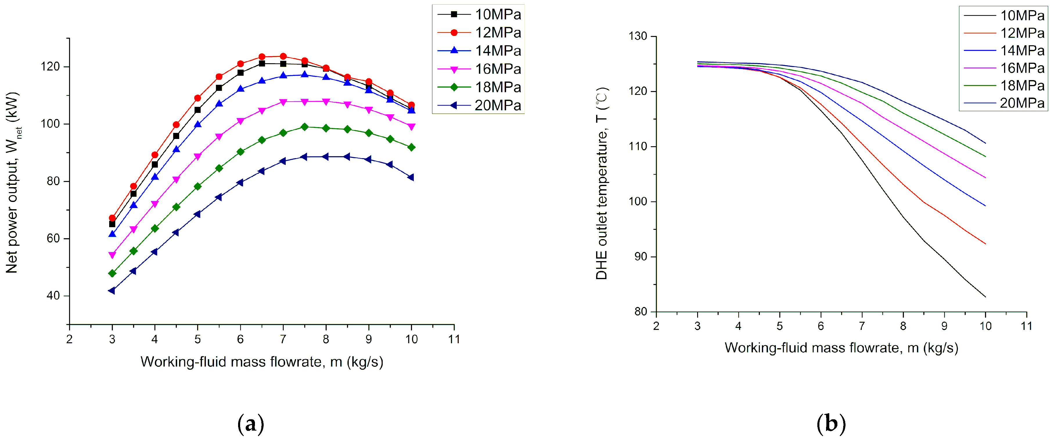
The working fluid R32/CO2 with an optimal mass fraction (as shown in Table 4) has been investigated for six different DHE inlet pressures (shown in the legend of Figure 3) under the conditions that the geofluid mass flowrate is 5 kg/s and the geofluid temperature is 130 °C. The effects of the working fluid’s flowrate and its DHE inlet pressure on the cycle’s net power output, as well as on the working-fluid’s DHE outlet temperature, are shown in Figure 3a,b respectively. As can be seen from Figure 3a, for each given DHE inlet pressure, there is a maximum net power output with a corresponding optimum working-fluid flowrate. The top curve (12 MPa curves) has the highest net power output with a value of about 120 kW when the working-fluid flowrate is 6.5 kg/s. Too high or too low DHE inlet pressure results in lower power output. In the scenario investigated here, the optimum DHE inlet pressure for obtaining maximum net power output is 11 MPa, as shown in Table 4.
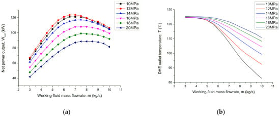
Figure 3.
Effect of working-fluid’s DHE inlet pressure on net power output (a), and on working-fluid’s DHE outlet temperature (b) with respect to the change of the working-fluid’s mass flowrate (mass fraction of R32/CO2 = 0.5/0.5, geofluid mass flowrate = 5 kg/s, geofluid temperature = 130 °C, DHE length = 300 m).
Figure 3b shows the effect of DHE inlet pressure on the DHE outlet temperature with respect to the change of the working-fluid’s mass flowrate. When the working-fluid flowrate is less than 4 kg/s, the DHE outlet temperature is almost same under the six investigated DHE inlet pressure conditions. This means that, when the working-fluid flowrate is small (less than 4 kg/s), the heat supply from the geofluid is big enough to enable the working fluid to approach the geofluid’s temperature.
When the working-fluid flowrate is greater than 4 kg/s, for any given DHE inlet pressure, the DHE outlet temperature starts to decline. As can be seen from Figure 3b, the decline rate of the DHE outlet temperature is different with the increase of the working-fluid flowrate; the greater the DHE inlet pressure, the smaller the decline rate, the higher the DHE outlet temperature.
It is worth pointing out that the higher DHE outlet temperature does not necessarily mean that the power cycle has a higher power output. This can be seen in Figure 3a, where the bottom power output curve corresponds to the highest DHE inlet pressure (20 MPa). Higher DHE inlet pressure means a higher pump work and, hence, a greater deduction in the net power output. Therefore, for a given geofluid temperature and mass flowrate, the working-fluid’s flowrate and its DHE inlet pressure should be optimized simultaneously.
4.4. Effect of Geofluid Mass Flowrate
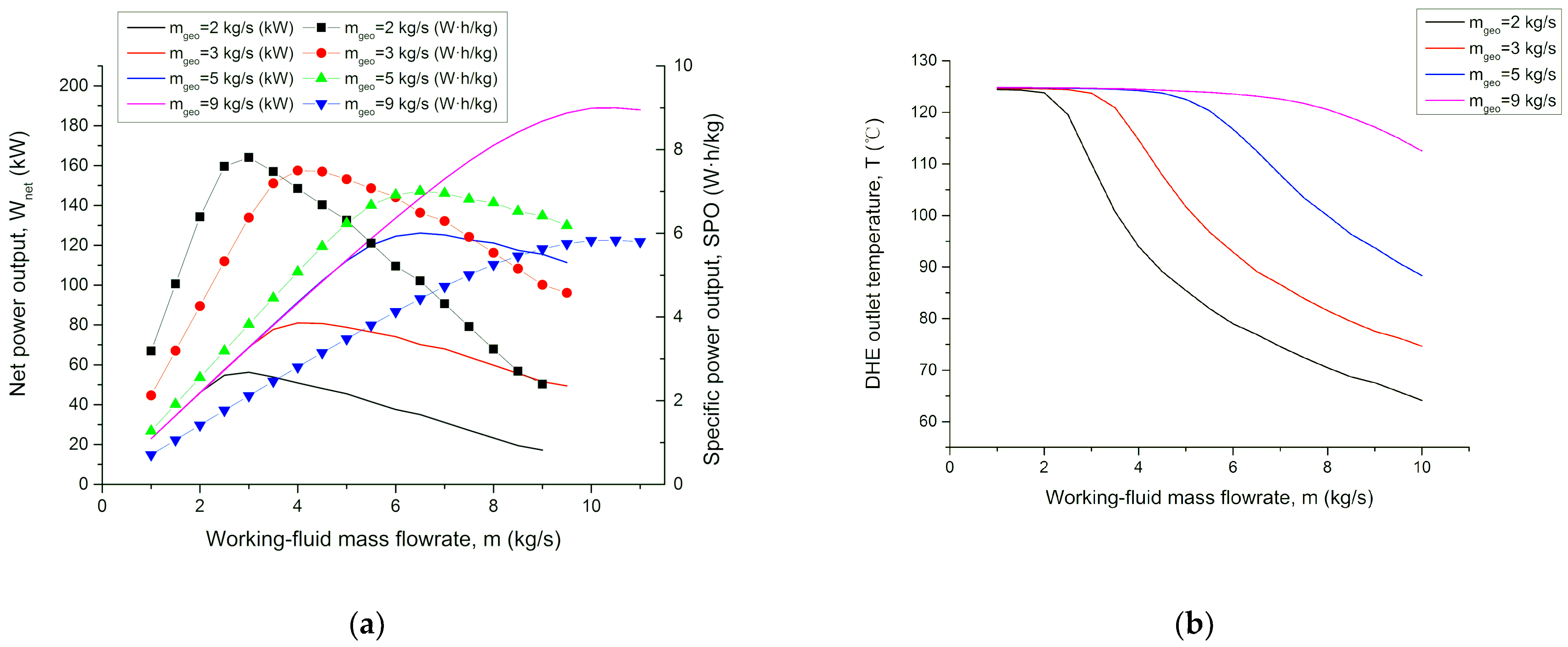
Figure 4 shows the effect of a geofluid mass flowrate on the cycle’s net power output and working-fluid’s DHE outlet temperature with respect to different working-fluid flowrates. The corresponding specific power output (power, in W, generated by a unit mass flowrate of geofluid, in kg/h) is also plotted in Figure 4a for discussion.
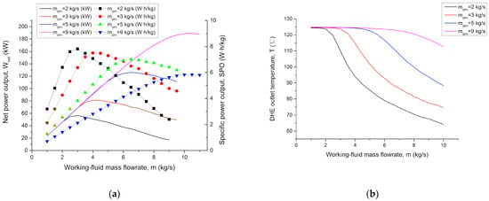
Figure 4.
Effect of geofluid flowrate on the net power output and corresponding specific power output (a), and working-fluid’s DHE outlet temperature (b) (working-fluid’s DHE inlet pressure = 11 MPa, mass fraction of R32/CO2 = 0.5/0.5, geofluid temperature = 130 °C, DHE length = 300 m).
Four different geofluid mass flowrates (2, 3, 5, and 9 kg/s) have been investigated under the conditions that the geofluid temperature is 130 °C, mass fraction of working fluid R32/CO2 is taken as 0.5/0.5 (optimal value), and working-fluid’s DHE inlet pressure is taken as 11 MPa (optimal value). The optimal values are seen in Table 4.
In Figure 4a, for each given geofluid flowrate, there is a corresponding optimal working-fluid flowrate. The higher the geofluid flow, the greater the optimal working-fluid flow. When the geofluid flowrate is 2 kg/s, the optimal working-fluid flowrate is 3 kg/s, corresponding to a specific power output of about 7.8 Wh/kg. Under the condition that the geofluid’s flowrate is 3 kg/s or 5 kg/s, the peak value of the specific power output in each case is gradually decreased. When the geofluid flowrate is 9 kg/s, there is an obvious decrease in the peak value of the specific power output. The specific power output, in this case, is only about 5.8 Wh/kg, with an optimal working-fluid flowrate of about 10 kg/s. A higher working-fluid flowrate (10 kg/s) means a higher pump work and, hence, a lower specific net power output. However, higher geofluid flowrate scenario shows a better off-design operation characteristic because the curve around its peak value is flatter. The optimal working-fluid flowrates can also be determined from the net power output curves. They are the same as those found using the specific power output curves. Different from the specific power output, the net power output increases as the geofluid flowrate becomes greater.
Figure 4b shows the variation of the working-fluid’s DHE outlet temperatures with respect to the working-fluid mass flowrate. When the geofluid flowrate is 9 kg/s, the working-fluid’s DHE outlet temperature is almost constant. Because the mass flowrate of the geofluid is high, the heat supply from the geofluid is so big that it enables the working fluid to approach the geofluid’s temperature. However, when the geofluid flowrate is not high (e.g., 2 kg/s), the outlet temperature starts to decline after the working-fluid flowrate is greater than 3 kg/s, with an obvious decrease rate, implying that an optimum match between the geofluid flowrate and the working-fluid mass flowrate becomes important when the geofluid flowrate is low.
4.5. Effect of the Downhole Heat Exchanger (DHE) Length
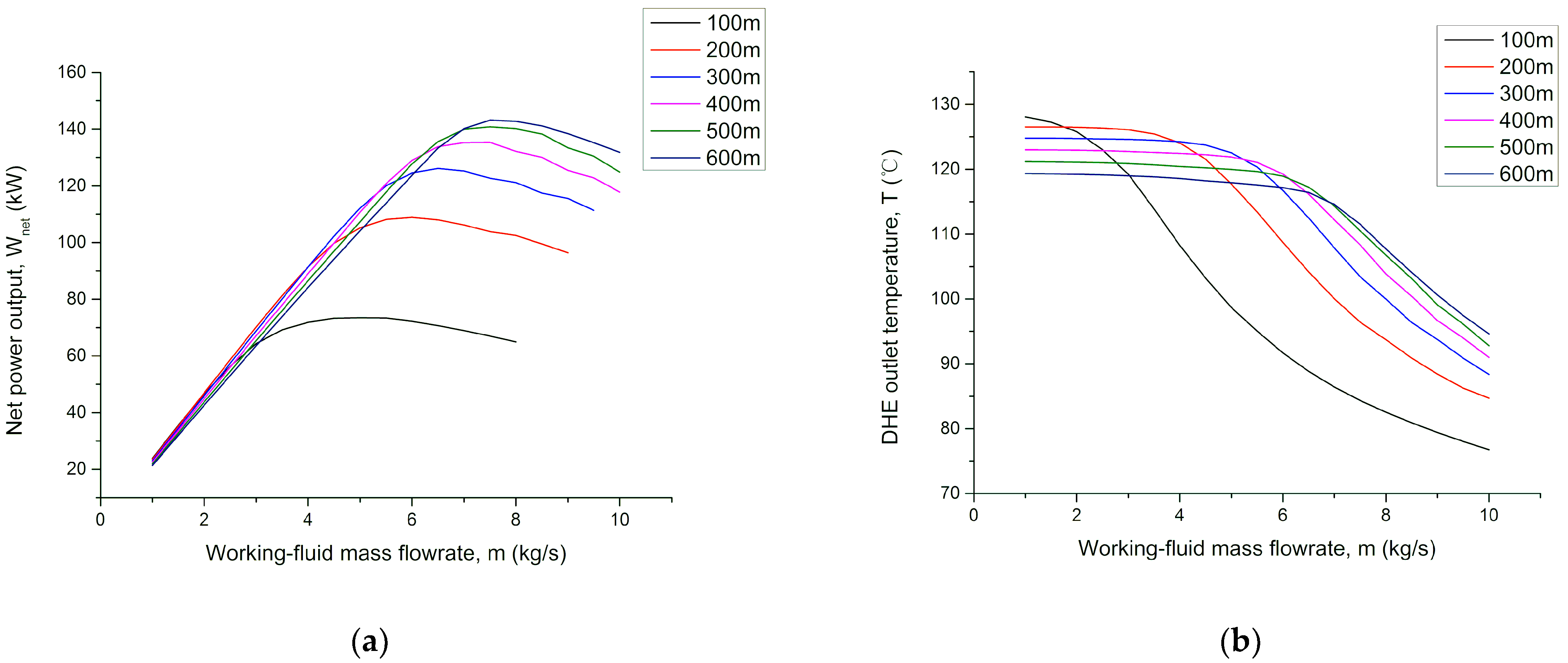
Figure 5a shows the change of net power output for a given DHE length with respect to the working-fluid flowrate. Six DHE lengths (100 m, 200 m, 300 m, 400 m, 500 m, and 600 m) were investigated under the conditions where the geofluid mass flowrate is 5 kg/s, the geofluid temperature is 130 °C, and the working-fluid’s DHE inlet pressure is 11 MPa. The mixture ratio of working fluid R32/CO2 is 0.5/0.5. It can be seen from Figure 5a that the length of DHE has an obvious influence on the net power output. For each given DHE length, the net power output has a peak value corresponding to an optimum working-fluid flowrate. The longer the DHE, the greater the optimum working-fluid flowrate, the higher the net power output. When the DHE is 100 m long, the optimum working-fluid flowrate is 5 kg/s with a maximum net power output of about 73 kW; whereas, when the DHE is 600 m long, the optimum working-fluid flowrate becomes 7.5 kg/s, corresponding to a maximum net power output of about 143 kW, which is almost two times the output when a 100 m-long DHE is used. Of course, in an engineering application, the optimum length of the DHE should be determined not only based on thermophysical analysis, but also on engineering economic analysis, with consideration of the costs of both DHE and the working fluid.
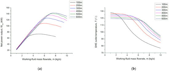
Figure 5.
Effect of the DHE length on net power output (a), and working-fluid’s DHE outlet temperature (b) (working-fluid DHE inlet pressure = 11 MPa, geofluid temperature = 130 °C, geofluid mass flowrate = 5 kg/s, mass fraction of R32/CO2 = 0.5/0.5).
The influence of the DHE length on the working-fluid’s DHE outlet temperature is shown in Figure 5b. It can be seen that, when the DHE is short (100 m), the working-fluid’s outlet temperature starts to decrease once the working-fluid mass flowrate is greater than 1 kg/s. When the DHE is long (600 m), the outlet temperature can maintain a constant value if the working-fluid’s flowrate is less than 8 kg/s. This is not difficult to understand. Shorter DHE means a less heat transfer area. Once the working-fluid flowrate increases to a certain value, the area of the short DHE is no longer enough to maintain the outlet temperature and, hence, there is a temperature decline, as shown in Figure 5b. Therefore, the longer the DHE, the more stable the outlet temperature. It is also seen from Figure 5b that, the longer the DHE, the lower the outlet temperature (in the stable section). Longer DHE means that more heat loss occurs in the inner pipe upward-flow and, hence, causes a slight decrease of the outlet temperature.
4.6. Performance Comparison between the Developed NPC and Conventional ORC
Thermodynamic performance (in terms of the net power output) has been compared between the developed novel power cycle (NPC) and the conventional organic Rankine cycle (ORC), which is widely used in geothermal power industry.
The ORC model of Lu et al. (2018) [31] has been used in this study. Based on the literature [32,33,34,35], R245fa and R601 were found to have better thermodynamic performance for the temperature range investigated and, hence, have been selected as the ORC’s working fluids for the comparative study here.
The key parameters of the ORC model are listed in Table 5. The heat source and heat sink parameters are shown in Table 6.
Table 5.
Key parameters of the ORC model.
Table 6.
Heat source and heat sink parameters.
The heat source inlet temperature for the ORC’s evaporator is the wellhead geofluid temperature, assuming that there is no 300-m downhole heat exchanger (DHE) in the well and that the geofluid flows upward in the well with heat transfer to the surroundings (formations) of the well through the wall of the wellbore until it reaches the wellhead. In this scenario, the wellhead geofluid temperature is some degree lower than the geofluid temperature at 300 m-depth in the well. Our numerical simulation for this scenario shows that the temperature of the geofluid that reaches the wellhead is at least 5 °C lower than that of the geofluid at the depth of 300 m in the well. Therefore, in this comparative study, the heat source inlet temperature for the ORC’s evaporator is set to be a temperature that is 5 °C lower than the geofluid temperature at the 300 m-depth.
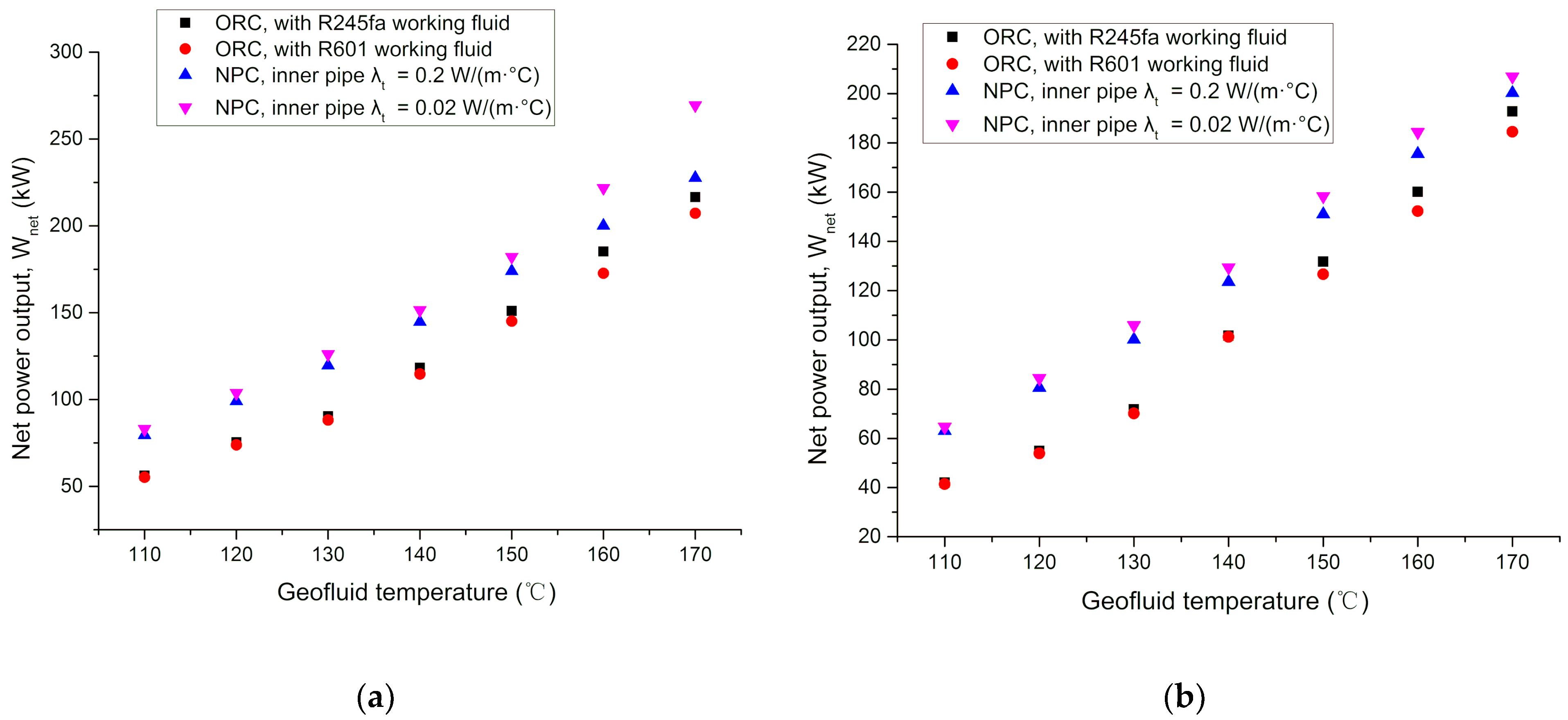
Figure 6 shows the comparison of net power output between the developed NPC and the conventional ORC that uses R245fa or R601 as working-fluid, respectively. Here, two cooling water temperature scenarios, 18 °C and 25 °C, were investigated. In order to analyze the influence of the thermal conductivity () of the DHE inner pipe on the power output, two values, 0.2 W/(m·°C) and 0.02 W/(m·°C), were considered in this simulation.
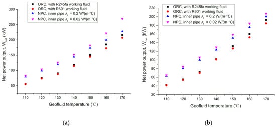
Figure 6.
Comparison of net power output between the developed novel power cycle (NPC) using R32/CO2 as working fluid and conventional ORC using R245fa or R601 as working fluid respectively, with two thermal conductivities, 0.2 W/(m·°C) and 0.02 W/(m·°C), of the DHE inner pipe being considered (geofluid mass flowrate = 5 kg/s, DHE length = 300 m). (a) Cooling water temperature is 18 °C. (b) Cooling water temperature is 25 °C.
The net power outputs of the four scenarios (shown in the legends of Figure 6) were simulated for geofluid temperatures ranging from 110 °C to 170 °C, using the heat source and heat sink parameters in Table 6, under the condition that the geofluid mass flowrate is 5 kg/s, and the DHE length is 300 m long.
As can be seen from Figure 6a,b, under any geofluid temperature conditions (from 110 °C to 170 °C), the net power output of the developed NPC is greater than that generated by the ORC using either R245 fa or R601 as working-fluid, no matter whether the cooling water temperature is low (18 °C) or high (25 °C), or the DHE inner pipe thermal conductivity is low (0.02 W/(m·°C)) or high (0.2 W/(m·°C)). This indicates that, under the heat source and heat sink conditions investigated, the developed NPC has a better thermodynamic performance than the conventional ORC. The advantage of using the developed NPC is more obvious when the geofluid temperature is low. The maximum net power output difference between the NPC and the ORC happens when geofluid temperature is 130 °C and NPC’s working fluid mass fraction (R32/CO2) is 0.5/0.5.
5. Conclusions
In this theoretical study, a power cycle with a unit capacity of several hundred kilowatts was configured and developed specifically for enhanced geothermal systems supplying geofluids with temperatures less than 170 °C. The thermodynamic performance of the developed novel power cycle (NPC) was analyzed in terms of the effects of the following important parameters: mass fraction of the mixture working fluids, working fluid’s flowrate and its DHE inlet pressure, geofluid flowrate, and length of the DHE. In addition, thermodynamic performance (in terms of the net power output) has been compared between the developed NPC and the conventional organic Rankine cycle (ORC). The following conclusions can be drawn from this study:
- (1)
- A transcritical power cycle with a higher net power output was developed using a suitable CO2-based mixture working fluid. Since the critical point of each used CO2-based mixture working fluid is higher than that of the pure CO2, a condensing process with a phase change can be realized. As a result, conventional condenser can be used, without being restricted to the use of costly large-area coolers, as in a CO2 Brayton cycle.
- (2)
- In the developed novel power cycle, an increasing-pressure endothermic process (instead of an isobarically endothermic process) was realized in a few-hundred-meters-long downhole heat exchanger (DHE) by making use of gravitational potential energy, which increases the cycle’s heat gain, as well as the working fluid’s pressure at the turbine inlet and, hence, increases the cycle’s power output.
- (3)
- In the downhole heat exchanger, the working fluid absorbs heat from the geofluid with a higher temperature at depth; thus, a higher outlet temperature of working fluid can be obtained, resulting in an increase of the working fluid’s temperature at the turbine inlet, contributing to a higher power output.
- (4)
- The increasing-pressure endothermic process in the DHE has a better match with the temperature change of the heat source (geofluid), as does the exothermic process in the condenser with the temperature change of the sink (cooling water), which reduces the heat transfer irreversibility and improves the power cycle efficiency.
- (5)
- For a given geofluid mass flowrate, the working-fluid’s flowrate and its DHE inlet pressure should be optimized simultaneously to get the maximum net power output. Higher geofluid mass flowrate usually corresponds to a higher optimum working-fluid flowrate.
- (6)
- From the thermophysical point of view, the longer the DHE, the greater the corresponding (optimum) working-fluid flowrate, the higher the net power output. In practice, however, the optimum length of the DHE should be determined based on engineering economics, considering the costs of both the DHE and the mixture working fluid.
- (7)
- In terms of the net power output, the developed NPC has a better thermodynamic performance than the conventional ORC for the geofluid temperature ranging from 110 °C to 170 °C. The lower the geofluid temperature, the more advantage of using the developed NPC.
- (8)
- Future research regarding an experimental study on the condensing process of the CO2-based mixture working fluid has been planned and will be carried out later.
Author Contributions
Conceptualization, C.G. and X.L.; methodology, C.G; software, C.G.; validation, C.G, X.L. and H.Y.; formal analysis, C.G., X.L.; investigation, C.G.; resources, X.L.; data curation, C.G., H.Y.; writing—original draft preparation, C.G.; writing—review and editing, X.L. and W.Z.; visualization, C.G. and J.Z.; supervision, X.L and J.W.; project administration, W.Z.; funding acquisition, X.L and J.W. All authors have read and agreed to the published version of the manuscript.
Funding
This research was funded by Ministry of Science and Technology of China (grant number 2018YFB1501805).
Institutional Review Board Statement
Not applicable.
Informed Consent Statement
Not applicable.
Data Availability Statement
Not applicable.
Acknowledgments
This work was supported by the National Key Research and Development Program of the 13th Five-Year Plan of China (grant number 2018YFB1501805).
Conflicts of Interest
The authors declare no conflict of interest.
Abbreviations
| Nomenclature | |
| H | Specific enthalpy, kJ/kg |
| j | Joule-Thomson coefficient |
| m | Working fluid mass flowrate, kg/s |
| Nu | Nusselt number, dimensionless |
| Pr | Prandtl number, dimensionless |
| Q | Heat transfer rate, kW |
| Raw | The thermal resistance between the geothermal water and the annulus, kW/(m2·°C) |
| Re | Reynolds number, dimensionless |
| Rta | The thermal resistance between the inner tube and the annulus, kW/(m2·°C) |
| Rw | The thermal resistance between the geothermal water and the formation, kW/(m2·°C) |
| t | Injection time, s |
| tD | Dimensionless injection time |
| W | The power output, kW |
| Wnet | Net power output, kW |
| α | Formation heat diffusivity(α = λe/(ce ρe)), m2/s |
| Subscripts | |
| 1,2,3… | State points |
| C | Condenser |
| cw | Cooling water |
| geo | Geofluid |
| h | Downhole heat exchanger |
| in | Inlet working fluid state |
| p | Pump |
| pinch | Pinch point |
| T | Turbine |
| Acronym | |
| CPG | CO2 Plume Geothermal |
| DHE | Downhole heat exchanger |
| EGS | Enhanced geothermal system |
| HDR | Hot Dry Rock |
| LEL | lower explosive limit |
| OEL | occupational exposure limit |
| ORC | Organic Rankine cycle |
| TRC | Transcritical Rankine cycle |
Appendix A
Appendix A.1. Flow Pressure Model of Downhole Heat Exchanger
In this model, the system is analyzed under steady conditions. The working-fluid flow is simplified as a one-dimensional flow and the mixtures is considered to be compressible. The diameters of the annulus, inner pipe, and wellbore are shown in Table 2. Under these conditions, the mass equation and the momentum equation can be simplified as [36]:
where is the density of the fluid, kg/m3; is the fluid velocity, m/s; z is flow path coordinate, m; g is the gravitational acceleration, m/s2;is the inclination angle; p is the pressure, Pa; is the shear stress, MPa; d is the equivalent diameter, m; is the cross-sectional area, m2. “+” represents the pressure change in annulus where flow direction is downward, and “−” represents the pressure change in inner pipe and wellbore where flow direction is upward.
Substituting Equation (A1) into Equation (A2) and replacing the friction term, the expression of fluid pressure can be obtained:
In the above formula, the Darcy friction factor is usually estimated based on experimental results. In this study, the correlations of the friction coefficients proposed by Wang et al. are used [37].
where Re is the Reynolds number, dimensionless; is the roughness of pipe wall, m.
Appendix A.2. DHE Temperature Field Model
According to the basic rules of heat transfer, the energy conservation equation of the working fluids can be written as follow:
where h is the specific enthalpy of fluid, m2/s2; q is the overall heat flow rate per unit length, J/(m·s). “+” represents the energy change in annulus where flow direction is downward, and “−” represents the energy change in inner pipe and wellbore where flow direction is upwards; other parameters have been defined earlier in Appendix A.1.
Combined with the mass Equation (A1), the energy conservation equation can be written as follow:
where w is the working-fluid flowrate, kg/s.
The specific enthalpy is given by the following formula [38]:
where is the specific heat capacity, J/(kg.K); is the Joule–Thomson coefficient, K/MPa.
Substituting the Equation (A7) into Equation (A6), the energy conservation equation can be written as follows:
is the heat produced by friction or viscous dissipation; is the heat produced by fluid expansion or compression; is the heat produced by the Joule–Thomson effect [39].
Appendix A.3. DHE Heat Transfer Model
The overall heat flow rate q can be expressed by the following formula [40]:
The flow heat transfer coefficient is expressed by the model of Dittus and Boelter [41], for the hot side n = 0.4, and for the cold side n = 0.3; d = 4∗AC/P is the equivalent diameter:
- (a)
- Heat transfer between the inner pipe and annulus
In this study, the thermal insulation layer between the inner-pipe inside wall and the inner-pipe outside wall is applied, as shown in Figure A1. The heat transfer between the inner pipe and annulus can be determined by
where is the total thermal resistance between the inner-pipe and the annulus, (m·°C)/W; is the overall heat transfer coefficient between the inner-pipe and the annulus, W/(m2·°C); is the inner radius of the inner-pipe inside wall, m; is the outer radius of the inner-pipe outside wall, m; is the convective heat transfer coefficient between the working fluid and the inner surface of the inner pipe, W/(m2·°C); is the heat conductivity of the inner pipe inside and outside walls, W/(m2·°C); is the inner radius of the inner-pipe outside wall, m; is the outer radius of the inner-pipe outside wall, m; is the heat conductivity of the insulation layer, W/(m2·°C); is the convective heat transfer coefficient between working fluid and the inner surface of the annulus, W/(m2·°C);
From the Figure A2, when the heat conductivity of the insulation layer is low, with values of 0.02, 0.002 and 0.0002 W/(m2·°C), the DHE outlet temperatures are very close, but when the heat conductivity is 0.2 W/(m2·°C), the DHE outlet temperature is about 5 degrees lower. Considering the technical economy and power output, the best heat conductivity would be 0.02 W/(m2·°C).

Figure A1.
Schematic diagram of the DHE model (Casing material: carbon steel).
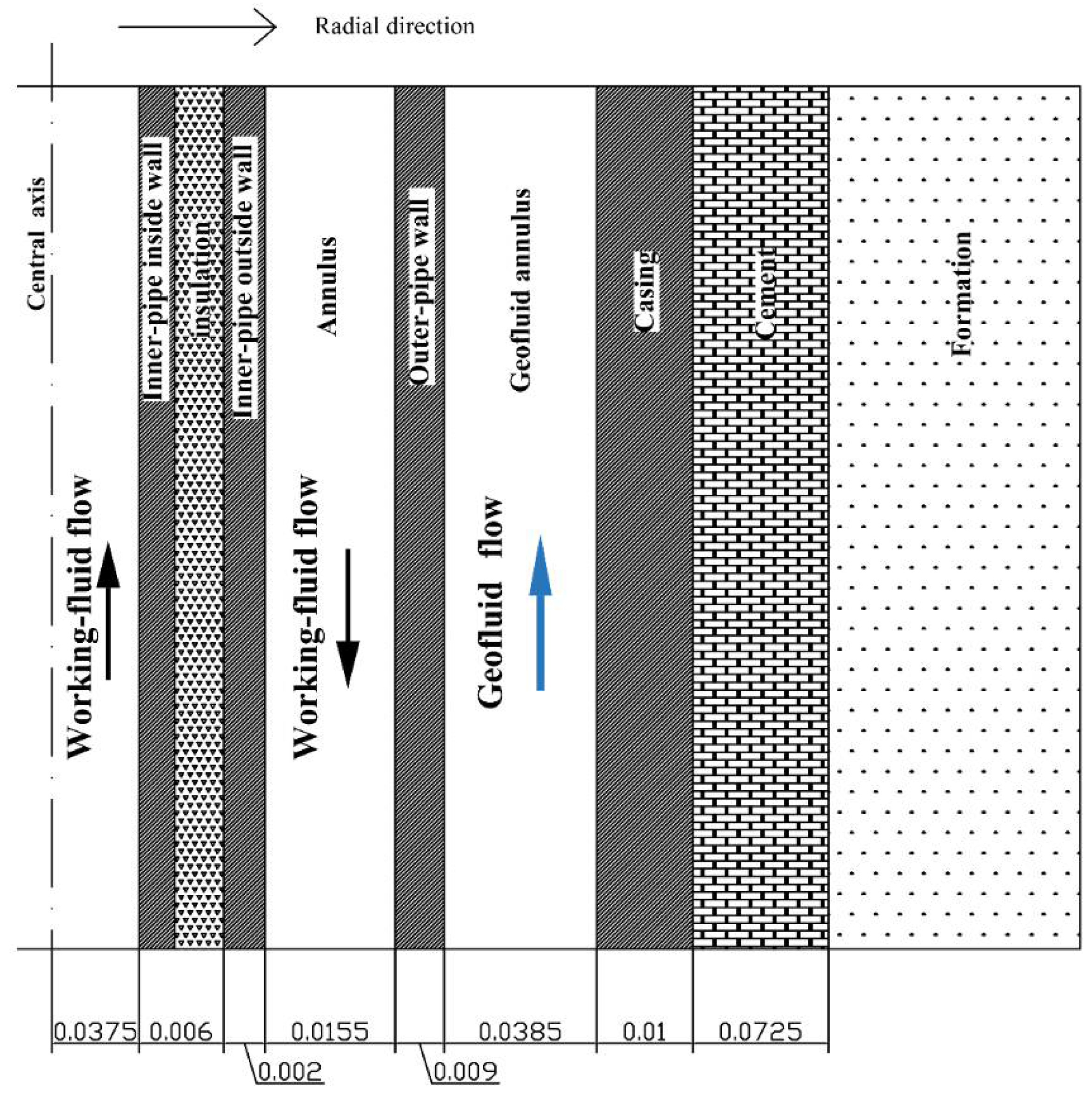
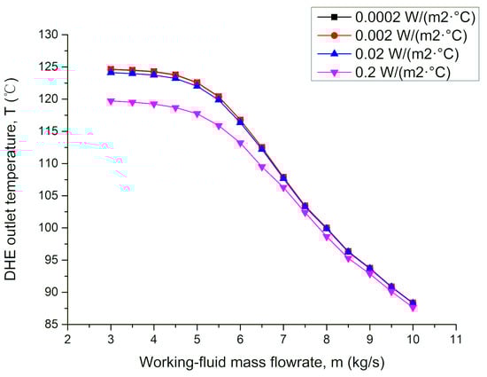
Figure A2.
Comparison of power cycle’s net power output in terms of using different heat conductivity of insulation layer (mixture ratio of working fluid = 0.5/0.5, geofluid mass flowrate = 5 kg/s, geofluid temperature = 130 °C, working-fluid’s DHE inlet pressure = 11 MPa, DHE length = 300 m).

- (b)
- Heat transfer between the annulus and geofluid
- (c)
- Heat transfer between the geofluid and formation
The heat transfer between the formation and the wellbore can be expressed as [42]:
where is the thermal conductivity of the formation, W/(m2·°C); is the formation temperature and decided by geothermal gradient, K; is the temperature of the outside wall of the wellbore, K; is the transient heat conduction function, dimensionless.
Cheng et al. considered the significance of wellbore heat capacity and proposed a new transient heat transfer function [43], which is then simplified as follows [44]:
where is dimensionless injection time.
In this paper, the injection time is set as 10,000 h; the can be neglected, so the above formula can be further simplified as follows:
The heat transfer between the wellbore and the formation can be determined by:
where Rw is the total thermal resistance between the geofluid and the formation, (m·°C)/W; Uw is the overall heat transfer coefficient between the geofluid and the formation, W/(m2·°C); rwi is the inner radius of the wellbore, m; rwo is the outer radius of the wellbore, m.
Appendix A.4. DHE Model Solution Procedure
The governing equations and the heat transfer model are coupled for iterative calculation. In this study, working fluid in the inner pipe and annulus, as well as the geofluid in the wellbore, are connected by heat transfer equations and governing equations. Each flow channel is divided into multiple cells along the flow direction. The thermal properties and flow parameters keep constant in each segment. All governing equations are converted into algebraic expressions in each cell. Through a series of integral iterative calculations, the temperature and pressure distributions of the flows can be obtained. Simulations were carried out using Python; REFPROP 9.0 was used to obtain the fluid thermal properties [45].
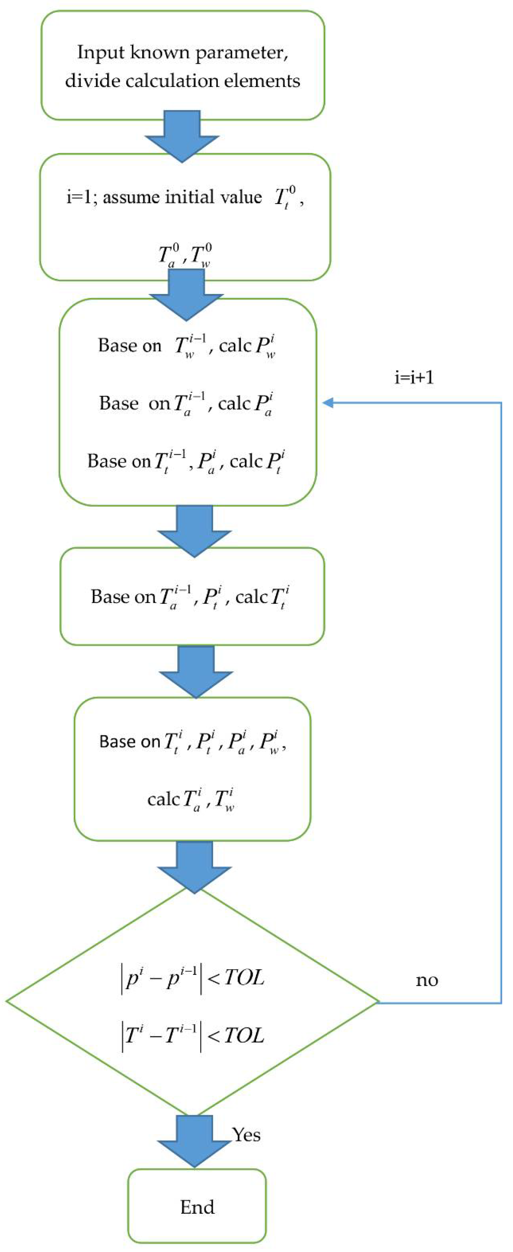
Figure A3 shows the flowchart of the simulation procedure, which can be summarized as follows:
(1) The working fluid in the inner pipe and annulus, as well as the geofluid in the wellbore, is divided into n cells along the flow direction; the position node is set as n.
(2) The temperature distributions of the working fluid in the inner pipe and in the annulus, and the temperature distribution of the geofluid, are all set as (N + 1) × 1 matrix.
(3) Along the flow direction, the geofluid pressure in each cell is calculated based on the temperature distribution and flow pressure Equation (A3).
(4) For a given annulus inlet pressure, the pressure distribution in each cell in the annulus is calculated along the flow direction based on the temperature distribution and the flow pressure Equation (A3).
(5) According to the annulus pressure distribution, the inlet pressure of the inner pipe can be obtained; the pressure distribution of the inner pipe can then be determined via the same method as described in step (4).
(6) The new temperature distribution of the inner pipe can be calculated based on the heat transfer model, the temperature Equation (A8), and the pressure and temperature distributions of the working fluid and geofluid.
(7) Based on the fluid’s temperature and pressure distributions in the inner pipe, the new temperature and pressure distribution of the annulus fluid and geofluid can be determined.
(8) Repeat (3)–(8) to obtain the temperature and the pressure distributions until the difference between the two adjacent steps is less than the expected error.
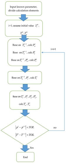
Figure A3.
Flow chart of the DHE simulation procedure.
References
- Yamankaradeniz, N.; Bademlioglu, A.H.; Kaynakli, O. Performance Assessments of Organic Rankine Cycle With Internal Heat Exchanger Based on Exergetic Approach. J. Energy Resour. Technol. 2018, 140, 102001. [Google Scholar] [CrossRef]
- Chen, H.; Goswami, D.Y.; Stefanakos, E.K. A review of thermodynamic cycles and working fluids for the conversion of low-grade heat. Renew. Sustain. Energy Rev. 2010, 14, 3059–3067. [Google Scholar] [CrossRef]
- El Haj Assad, M.; Aryanfar, Y.; Javaherian, A.; Khosravi, A.; Aghaei, K.; Hosseinzadeh, S.; Pabon, J.; Mahmoudi, S.M.S. Energy, exergy, economic and exergoenvironmental analyses of transcritical CO2 cycle powered by single flash geothermal power plant. Int. J. Low-Carbon Technol. 2021, 16, 1504–1518. [Google Scholar] [CrossRef]
- Khosravi, A.; Syri, S.; Zhao, X.; Assad, M.E.H. An artificial intelligence approach for thermodynamic modeling of geothermal based-organic Rankine cycle equipped with solar system. Geothermics 2019, 80, 138–154. [Google Scholar] [CrossRef]
- Pasinato, H.D. Working Fluid Dependence on Source Temperature for Organic Rankine Cycles. J. Energy Resour. Technol. 2019, 142, 012103. [Google Scholar] [CrossRef]
- Karellas, S.; Schuster, A. Supercritical Fluid Parameters in Organic Rankine Cycle Applications. Int. J. Thermodyn. 2008, 11, 101–108. [Google Scholar]
- Zhang, X.R.; Yamaguchi, H.; Fujima, K.; Enomoto, M.; Sawada, N. Study of solar energy powered transcritical cycle using supercritical carbon dioxide. Int. J. Energy Res. 2006, 30, 1117–1129. [Google Scholar] [CrossRef]
- Zhang, X.; Yamaguchi, H.; Fujima, K.; Enomoto, M.; Sawada, N. Theoretical analysis of a thermodynamic cycle for power and heat production using supercritical carbon dioxide. Energy 2007, 32, 591–599. [Google Scholar] [CrossRef]
- Chen, Y.; Lundqvist, P.; Johansson, A.; Platell, P. A comparative study of the carbon dioxide transcritical power cycle compared with an organic rankine cycle with R123 as working fluid in waste heat recovery. Appl. Therm. Eng. 2006, 26, 2142–2147. [Google Scholar] [CrossRef]
- Adams, B.M.; Kuehn, T.H.; Bielicki, J.M.; Randolph, J.B.; Saar, M.O. On the importance of the thermosiphon effect in CPG (CO2 plume geothermal) power systems. Energy 2014, 69, 409–418. [Google Scholar] [CrossRef]
- Sun, X.; Liao, Y.; Wang, Z.; Sun, B. Geothermal exploitation by circulating supercritical CO2 in a closed horizontal wellbore. Fuel 2019, 254, 115566. [Google Scholar] [CrossRef]
- Adams, B.; Kuehn, T.H.; Bielicki, J.; Randolph, J.B.; Saar, M.O. A comparison of electric power output of CO2 Plume Geothermal (CPG) and brine geothermal systems for varying reservoir conditions. Appl. Energy 2015, 140, 365–377. [Google Scholar] [CrossRef]
- Amaya, A.; Scherer, J.; Muir, J.; Patel, M.; Higgins, B. GreenFire Energy Closed-Loop Geothermal Demonstration using Supercritical Carbon Dioxide as Working Fluid. In Proceedings of the 45th Workshop on Geothermal Reservoir Engineering, Stanford, CA, USA, 10–12 February 2020; Available online: https://pangea.stanford.edu/ERE/db/GeoConf/papers/SGW/2020/Higgins.pdf (accessed on 22 December 2020).
- Xia, J.; Wang, J.; Zhang, G.; Lou, J.; Zhao, P.; Dai, Y. Thermo-economic analysis and comparative study of transcritical power cycles using CO2-based mixtures as working fluids. Appl. Therm. Eng. 2018, 144, 31–44. [Google Scholar] [CrossRef]
- Dai, B.; Li, M.; Ma, Y. Thermodynamic analysis of carbon dioxide blends with low GWP (global warming potential) working fluids-based transcritical Rankine cycles for low-grade heat energy recovery. Energy 2014, 64, 942–952. [Google Scholar] [CrossRef]
- Wu, C.; Wang, S.-S.; Jiang, X.; Li, J. Thermodynamic analysis and performance optimization of transcritical power cycles using CO2-based binary zeotropic mixtures as working fluids for geothermal power plants. Appl. Therm. Eng. 2017, 115, 292–304. [Google Scholar] [CrossRef]
- Matthews, H.B. Gravity Head Geothermal Energy Conversion System. U.S. Patent No. 4,077,220, 7 March 1978. [Google Scholar]
- Hogarth, R.A.; Daniel, B. Flow performance of the Habanero EGS closed loop. In Proceedings of the World Geothermal Congress, Melbourne, Australia, 16–24 April 2015. [Google Scholar]
- Hogarth, R.; Holl, H.G. Lessons learned from the Habanero EGS Project. Trans. Geotherm. Resour. Counc. 2017, 41, 865–877. [Google Scholar]
- Calm, J.M.; Hourahan, G.C. Physical, safety, and environmental data for current and alternative refrigerants. In Proceedings of the 23rd international congress of refrigeration (ICR2011), Prague, Czech Republic, 21–26 August 2011; pp. 4120–4141. [Google Scholar]
- Heberle, F.; Preißinger, M.; Brüggemann, D. Zeotropic mixtures as working fluids in Organic Rankine Cycles for low-enthalpy geothermal resources. Renew. Energy 2012, 37, 364–370. [Google Scholar] [CrossRef]
- Bell, I.H.; Lemmon, E.W. Automatic Fitting of Binary Interaction Parameters for Multi-fluid Helm-holtz-Energy-Explicit Mixture Models. J. Chem. Eng. Data 2016, 61, 3752–3760. [Google Scholar] [CrossRef]
- Chys, M.; Van Den Broek, M.; Vanslambrouck, B.; De Paepe, M. Potential of zeotropic mixtures as working fluids in organic Rankine cycles. Energy 2012, 44, 623–632. [Google Scholar] [CrossRef]
- Saleh, B.; Koglbauer, G.; Wendland, M.; Fischer, J. Working fluids for low-temperature organic Rankine cycles. Energy 2007, 32, 1210–1221. [Google Scholar] [CrossRef]
- Yin, H.; Sabau, A.; Conklin, J.C.; McFarlane, J.; Qualls, A.L. 2013. Mixtures of SF6–CO2 as working fluids for geothermal power plants. Appl. Energy 2013, 106, 243–253. [Google Scholar] [CrossRef]
- Larjola, J. Electricity from industrial waste heat using high-speed organic Rankine cycle (ORC). Int. J. Prod. Econ. 1995, 41, 227–235. [Google Scholar] [CrossRef]
- Mondal, S.; De, S. 2015 CO2 based power cycle with multi-stage compression and intercooling for low temperature waste heat recovery. Energy 2015, 90, 1132–1143. [Google Scholar] [CrossRef]
- Wang, J.; Guo, Y.; Zhou, K.; Xia, J.; Li, Y.; Zhao, P.; Dai, Y. Design and performance analysis of compressor and turbine in supercritical CO2 power cycle based on system-component coupled optimization. Energy Convers. Manag. 2020, 221, 113179. [Google Scholar] [CrossRef]
- Liu, Z.; Luo, W.; Zhao, Q.; Zhao, W.; Xu, J. Preliminary Design and Model Assessment of a Supercritical CO2 Compressor. Appl. Sci. 2018, 8, 595. [Google Scholar] [CrossRef] [Green Version]
- Dyreby, J.; Klein, S.; Nellis, G.; Reindl, D. Design Considerations for Supercritical Carbon Dioxide Brayton Cycles with Recompression. J. Eng. Gas Turbines Power 2014, 136, 101701. [Google Scholar] [CrossRef]
- Lu, X.; Zhao, Y.; Zhu, J.; Zhang, W. Optimization and applicability of compound power cycles for enhanced geothermal systems. Appl. Energy 2018, 229, 128–141. [Google Scholar] [CrossRef]
- He, C.; Liu, C.; Gao, H.; Xie, H.; Li, Y.; Wu, S.; Xu, J. The optimal evaporation temperature and working fluids for subcritical organic Rankine cycle. Energy 2012, 38, 136–143. [Google Scholar] [CrossRef]
- Hung, T.; Wang, S.; Kuo, C.; Pei, B.; Tsai, K. A study of organic working fluids on system efficiency of an ORC using low-grade energy sources. Energy 2010, 35, 1403–1411. [Google Scholar] [CrossRef]
- Mago, P.J.; Chamra, L.M.; Somayaji, C. Performance analysis of different working fluids for use in organic Rankine cycles. Proc. Inst. Mech. Eng. Part A J. Power Energy 2007, 221, 255–263. [Google Scholar] [CrossRef]
- Guo, T.; Wang, H.; Zhang, S. Comparative analysis of CO 2-based transcritical Rankine cycle and HFC245fa-based subcritical organic Rankine cycle using low-temperature geothermal source. Sci. China Technol. Sci. 2010, 53, 1638–1646. [Google Scholar] [CrossRef]
- Hasan, A.R.; Kabir, C.S.; Sarica, C. Fluid Flow and Heat Transfer in Wellbores; Society of Petroleum Engineers Richardson: Richardson, TX, USA, 2002. [Google Scholar]
- Wang, Z.; Sun, B.; Wang, J.; Hou, L. Experimental study on the friction coefficient of supercritical carbon dioxide in pipes. Int. J. Greenh. Gas Control. 2014, 25, 151–161. [Google Scholar] [CrossRef]
- Hasan, A.; Kabir, C. A mechanistic model for computing fluid temperature profiles in gas-lift wells. SPE Prod. Facil. 1996, 11, 179–185. [Google Scholar] [CrossRef]
- Li, X.; Li, G.; Wang, H.; Tian, S.; Song, X.; Lu, P.; Wang, M. A unified model for wellbore flow and heat transfer in pure CO2 injection for geological sequestration, EOR and fracturing operations. Int. J. Greenh. Gas Control. 2017, 57, 102–115. [Google Scholar] [CrossRef]
- Hasan, A.; Kabir, S. Wellbore heat-transfer modeling and applications. J. Pet. Sci. Eng. 2012, 86-87, 127–136. [Google Scholar] [CrossRef]
- Dittus, F.W.; Boelter, L.M.K. Heat transfer in automobile radiators of the tubular type. Int. Commun. Heat Mass Transf. 1985, 12, 3–22. [Google Scholar] [CrossRef]
- Hasan, A.R.; Kabir, C.S. Heat transfer during two-Phase flow in Wellbores; Part I—Formation temperature. In SPE Annual Technical Conference and Exhibition; OnePetro: Richardson, TX, USA, 1991. [Google Scholar]
- Cheng, W.-L.; Huang, Y.-H.; Lu, D.; Yin, H.-R. A novel analytical transient heat-conduction time function for heat transfer in steam injection wells considering the wellbore heat capacity. Energy 2011, 36, 4080–4088. [Google Scholar] [CrossRef]
- Cheng, W.; Nian, Y. High precision approximate solution of transient heat-conduction time function of wellbore heat transfer. Huagong Xuebao/CIESC J. 2013, 64, 1561–1565. [Google Scholar] [CrossRef]
- Lemmon, E.W.; Huber, M.L.; McLinden, M.O. NIST reference fluid thermodynamic and transport properties–REFPROP. NIST Stand. Ref. Database 2002, 23, v7. [Google Scholar]
Publisher’s Note: MDPI stays neutral with regard to jurisdictional claims in published maps and institutional affiliations. |
© 2022 by the authors. Licensee MDPI, Basel, Switzerland. This article is an open access article distributed under the terms and conditions of the Creative Commons Attribution (CC BY) license (https://creativecommons.org/licenses/by/4.0/).