1. Introduction
Clustering is an informatics technique that allows practitioners to focus attention on a few important factors in a process. In clustering, the analyst takes unsupervised or untagged data and divides it into what are intended to be intuitive groupings. Then, knowledge is gained about the whole dataset or “corpus” and any new items can be automatically assigned to groups. As a result, clustering can provide a data-driven prioritization for quality issues relevant to allocating limited attention and resources. Informatics professionals are asked now more than ever to be versant in using the information technology revolution [
1,
2,
3]. This revolution exposed practitioners to large databases of images (and texts) that provided insights into quality issues. Practitioner might easily create clustering or logistic regression models using the rating field. Yet, the practitioner generally has no systematic technique for analyzing the freestyle text or image. This is true even while the text or image clearly contains much relevant information for causal analysis [
4,
5].
This article proposes methods with sufficient generality to provide the ability to apply the analysis either for images or texts. Each image (or record) could correspond to more than a single quality issue. For example, one part of a weld image might include nonconformity at the same time reveals another type of nonconformity. In addition, it might be too expensive to go through all the images (or documents), to identify the quality issues manually. The purpose of this article is to propose a new way to identify quality issues combined with different images (or texts) by generating clustering charts to prioritize quality issues. For example, if the engineers knew that type 1 defects were much more common than the other types, they could focus on the techniques relevant to type 1 for quality improvement and address the most important issues of that type. This new method will require relatively little effort from practitioners compared with manually tagging all or a large fraction of the data.
Even while the information technology revolution is exposing practitioners to new types of challenges it is also making some relevant estimation methods like Bayesian analysis easier [
6,
7,
8,
9]. One aspect that many Bayesian applications have in common is that they do not apply informative prior distributions. This is presumably because, in all these cases, the relevant practitioners did not have sufficient knowledge before analysis that they could confidently apply to make the derived models more accurate. The phrase “supervised” data analysis refers to the case in which all the data used for analysis has been analyzed by subject matter experts (SMEs) and categorized into classes by cause or type. Past analyses of text or image data in quality contexts have focused on supervised data analyses [
10,
11]. Yet, more generally perhaps, datasets are sufficiently large that having personnel read or observe all or even a significant fraction of the articles or images and categorize them into types is prohibitively expensive. Apley and Lee [
12] developed a framework for integrating on-line and off-line data which is also presented in this article. This framework did not include new types and convenient types of data. Here, we are seeking to have the data presented in different forms.
The approach proposed in this paper is apparently the first to model replication and other errors in both high-level expert and “low-level” data for unstructured multi-field text or image modeling for image analysis. Allen, Xiong and Afful-Dadzie [
4] did this for text data. The practical benefit that we seek is to permit the user to edit the cluster or topic definitions easily. In general, Bayesian mixture models provide clusters with interpretable meaning and are generalizations of latent semantic indexing approaches [
13]. The Latent Dirichlet Allocation (LDA) method [
13] has received a lot of attention because the cluster definitions derived often seem interpretable. Yet, these definitions may seem inaccurate and disagree with expert judgement. Most recently, many researchers have further refined Bayesian mixture models to make the results even more interpretable and predictive [
14,
15,
16,
17,
18]. This research has generally caused the complexity of the models to grow together with the number of estimated parameters. The approach taken here is to use a relatively simple formulation and attempt to mitigate the misspecification issues by permitting user interaction through the high-level data.
To generate clustering models to analyze image data, we must identify clusters definitions which is the most challenging step, tally the total proportions of all the images associated with each cluster, sort the tallies and bar chart the results. Another objective we have for this article is to compare the proposed clustering methods with alternatives methods that have been used before. This follows because those methods require that the cluster definitions are pre-defined, all pixels in each image relate to a single cluster, and a “training set” of images have been pre-tagged or supervised [
19,
20,
21]. For two simulated numerical examples, we compare the proposed clustering methods with three relevant alternatives: Latent Dirichlet Allocation [
13,
22,
23], “fuzzy c means” clustering methods [
24,
25] and pre-processing using principle components analysis followed by fuzzy c means clustering [
26]. Apparently, comparisons of a similar scope do not appear in the image analysis literature which generally focuses on the goal of retrieving relevant documents. Our research here applies the existing results for text analysis [
4]. To generate helpful prioritizations, we need the estimated topic definitions and proportions to be accurate. Therefore, we also propose new measures of model accuracy relevant to our goals for image analysis.
Next section, we describe the laser welding image problem that motivates the Expert Refined Topic (ERT) modeling methods for image analysis. The motivation relates to the issue that none of the topics or clusters identified directly corresponds to the issues defined in the American National Standard Institute (ANSI) conformance standards.
Motivating Problem: Laser Welding
Many manufacturing processes involve images used to evaluate the conformance of parts to standards [
6,
27,
28].
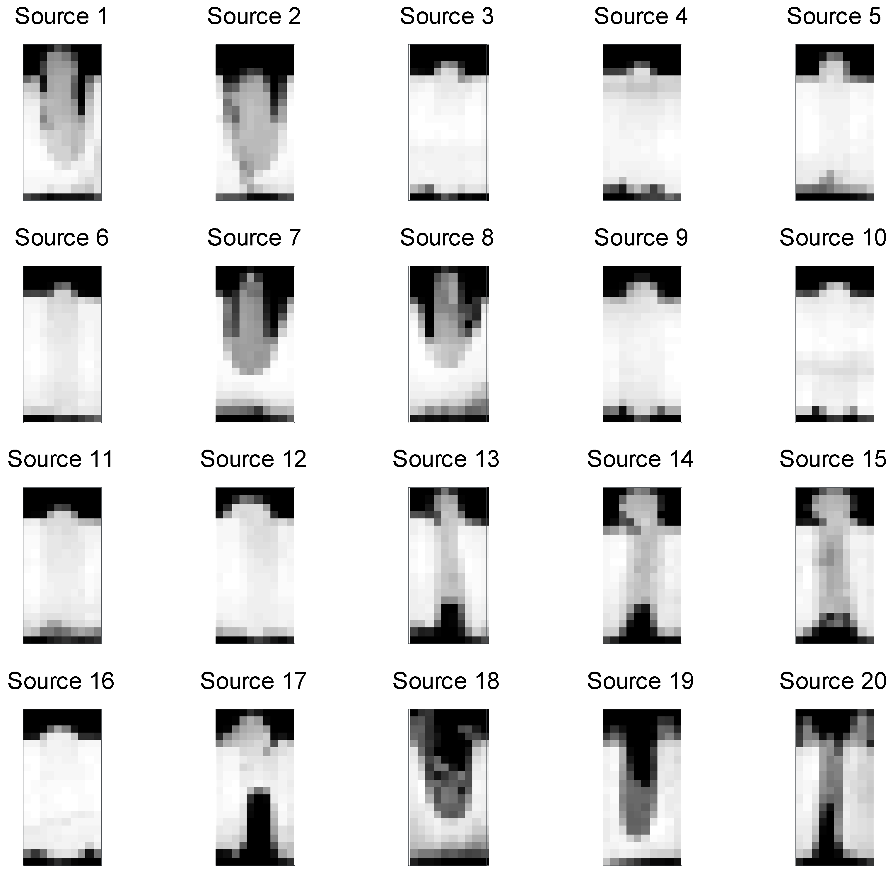
Figure 1 shows digital images from 20 laser aluminum alloy parts, which were sectioned and photographed. The first image (Source 1) can be represented as a vector of pixel numbers with added counts for the darker pictures. This is given in
Table 1(a). This “bag of words” representation is common to topic models but has drawbacks including the document lengths being related to the number of distinct levels of grayscale [
13].
Table 1(b) includes the inputs from our methods which are described in
Section 4. In this example, the number of images is small enough such that supervision of all images manually is not expensive. In addition, generating the image data of cut sections of the welds is expensive because the process is destructive, i.e., the sectioned parts cannot be sold. Generally, manufacturing situations that involve nondestructive evaluation can easily generate thousands of images or more. In these situations, human supervision of even a substantial fraction of these images is prohibitively expensive. Our problem statement is to create topic definitions and an automatic system that can cluster items (weld images) into groups that conform to pre-known categories while spanning the set of actual items. We seek to do this with a reasonable request of information from the welding engineers involved.
In addition, in
Figure 1, the images may seem blurry. This follows because they are 20 × 10 = 200 pixels because it was judged that such simple images are sufficient for establishing conformance and are easier to store and process than higher resolution images. We will discuss the related issues of resolution and gray scale bit selection after the methods have been introduced. In the next section, we review the methods associated with Latent Dirichlet Allocation (LDA) [
13].
LDA is perhaps the most widely cited method relevant to unsupervised image processing. The cluster or “topic” definitions identified by LDA can themselves be represented as images. They are defined formally by the posterior means for the pixel or “word” probabilities associated with each topic.
Figure 2 shows the posterior mean topic definitions from applying 3000 iterations of collapsed Gibbs sampling using our own C++ implementation. The topic definitions are probabilities that each pixel would be selected in a random draw or word. The fact that they can be interpreted themselves as images is a positive properties of topic models such as LDA.
At present, there are many methods to determine the number of topics in the fitted model [
29,
30,
31,
32,
33].
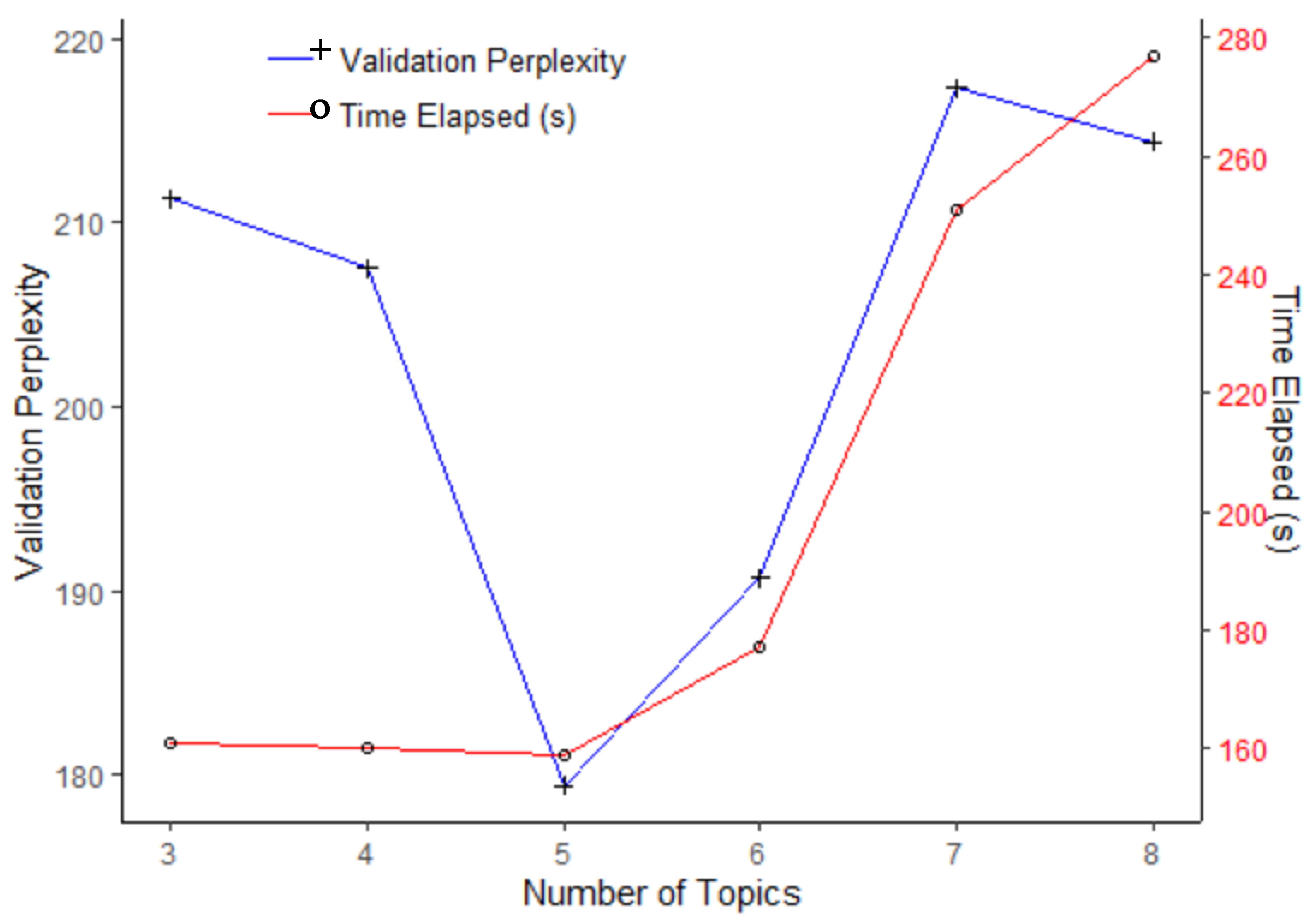
Appendix B describes the selection of five topics for this problem.
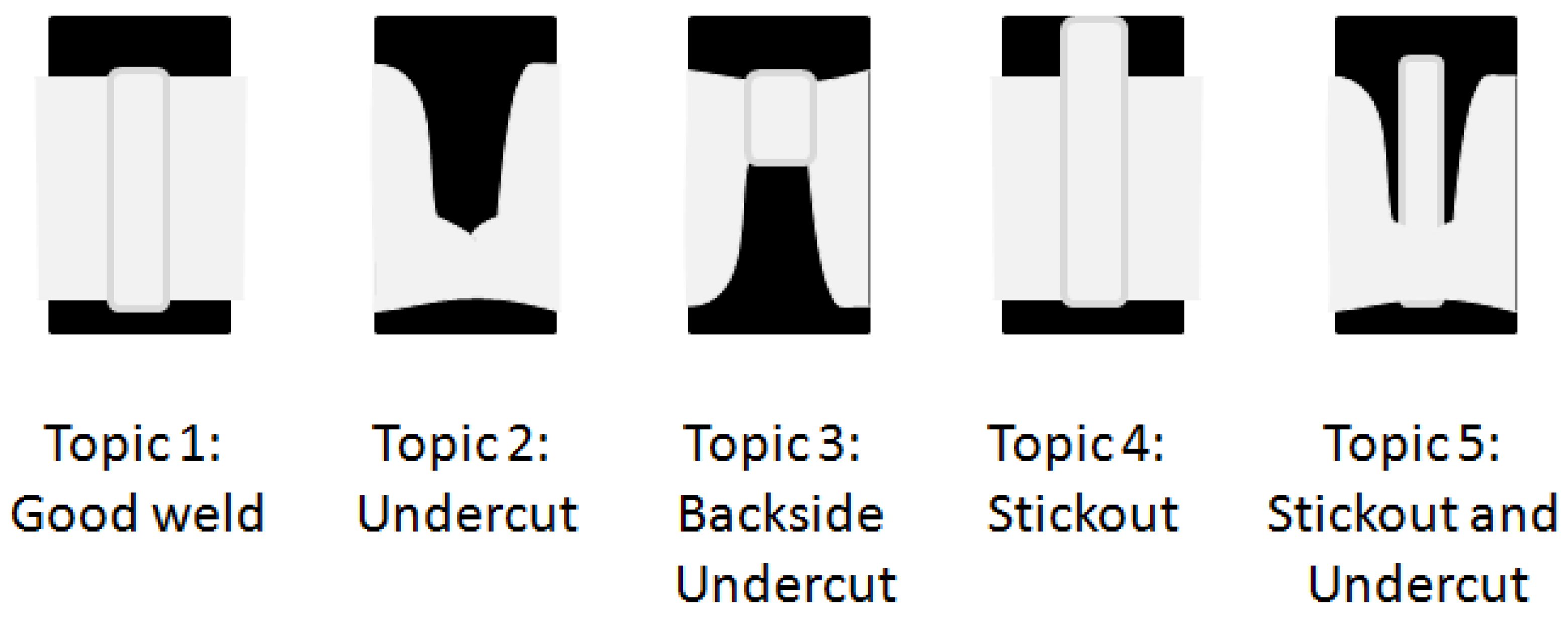
Figure 3 illustrates the most relevant international American National Standard Institute/American Welding Society (ANSI/AWS) conformance issues for the relevant type of aluminum alloy pipe welds [
30]. These were hand drawn but they are quite standard and illustrate the issues an arc welding quality inspector might look for in examining images from a sectioned part.
If it were possible to have the topic definitions correspond closely with these known conformance issues, then the resulting model could not only assign the probability that welds are conforming but also provide the probabilities of specific issues applying. In addition, the working vocabulary of welding engineers including “undercut”, “penetration” and “stickout” could be engaged to enhance interpretability [
34]. The primary purpose of this article is to propose methods that provide recourse for users to shape the topics directly without tagging individual images.
Section 2 describes the related works. In
Section 3, we describe the notation and review the Latent Dirichlet Allocation methods whose generalization forms the basis of ERT models, which are then proposed for image analysis. The ERT model application involves a step in which “handles” are applied using thought experiments to generate high-level data in
Section 4.
Then we describe the “collapsed” Gibbs sampling formulation, which permits the exploration of databases involving thousands of images or documents. The proposed formulation is exact in certain cases that we describe and approximate in others, with details provided in
Appendix A. In
Section 5, two numerical examples illustrate the benefits for cases in which the ground truth is known. In
Section 6, we illustrate the potential value of the method in the context of a real-world, laser welding image application and conclude with a brief discussion of the balance between high-level and ordinary data in modeling in
Section 7.
4. Methods
Widely acknowledged principles for modeling and automation include that the models should be both “observable” so that the users can see how they operate and “directable” so that users can make adjustments on a case-by-case basis [
40]. We argue that topic models are popular partly because they are simpler and, therefore, more observable than alternative models, which might include expert systems having thousands of ad hoc, case-specific rules. Yet, the only “directability” in topics models comes through the prior parameters
α and
β. Specifically, adjustments to
α and
β only control the degree of posterior uniformity in the document-topic probabilities and the degree of uniformity of the topic-word probabilities, respectively. Therefore,
α and
β are merely Bayesian shrinkage parameters.
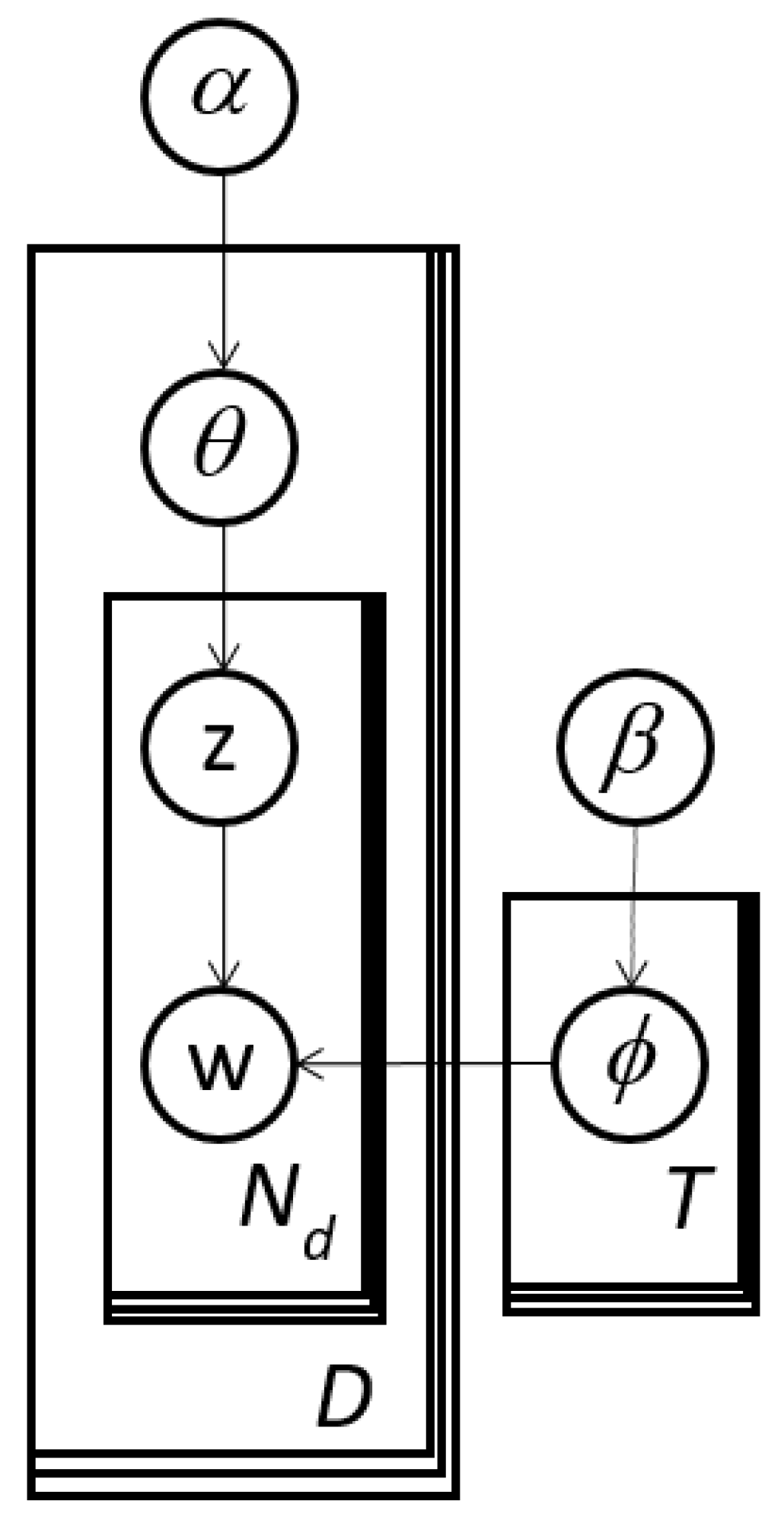
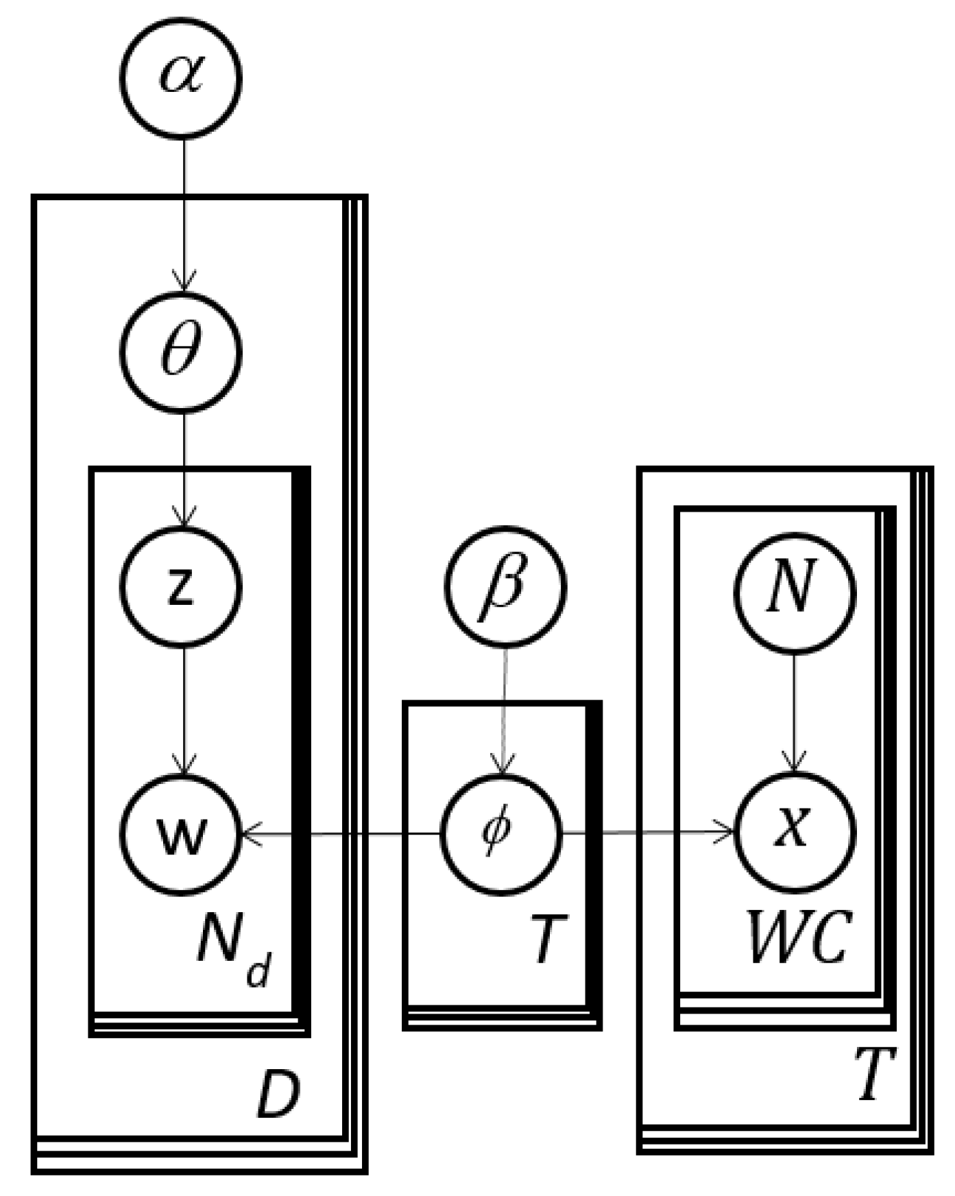
We propose for image analysis the subject matter expert refined topic (ERT) model in
Figure 5 to make the LDA topic model more directable. The left-hand-side is identical to LDA in
Figure 4, which has multinomial response data,
w. The right-hand-side is new and begins with the arrow from
ϕ to
x. This portion introduces binomially distributed response data,
for
t = 1, …,
T and
c = 1, …,
WC. The
represent the number of times for a given topic,
t, word
c is selected in
trials. Therefore,
is a sample size for thought experts.
Like LDA, ERT models are merely distributions to be fit to data. The usual data points are assumed to be random (multinomial) responses (
ws) which are part of the LDA “wing” (left-hand-side of
Figure 5). The inputs from the experts (or just users) are random counts (
xs) from imaged “thought” experiments on the right-hand-side (right wing) of
Figure 5.
In our examples, we use = 1M for cases when the expert or user is confident that they want to remove a word (“zap”). Smaller sizes, e.g., = 1000, might subjectively indicate less confidence or weight in the expert data. In our preliminary robustness studies, sample sizes below 1M often had surprisingly little effect for zapping. Note also that the choice of in the model is arbitrary and many combinations of topics t and words c can have .
We refer to the right-hand-side portions in
Figure 4 (the rectangles including
N and
x) as handles because they permit users to interact with the model in a novel way in analogy to using a carrying appendage on a pot. These experiments are “designed” because the analyst can plan and direct the data collection. These binomial thought experiments have relatively high leverage on specific latent variables, i.e.,
ϕ. We propose that users can apply this model in two or more stages. After initially applying ordinary LDA, the user can study the results and then gather data from experiments involving potentially subject matter experts (SMEs) leading to Expert Refined Topic (ERT) models or Subject Matter Expert Refined Topic (SMERT) models. Note that a similar handle could be added to any other topic model with a similarly defined topic definition matrix,
ϕ.
The so-called “latency experiments” [
4] could be literal as having the expert create prototype images for each topic and then extracting the binomial counts from these images. Alternatively, the experiments could be simple thought experiments, i.e., out of several trials, how many draws would you expect to result in a certain pixel image being derived? One difference than makes ERT models different for images as compared with text [
4] is that zapping is essentially an “eraser” for the topic definitions. This could even be accomplished using eraser icons on touch screens.
As an example, consider that an expert might be evaluating topic 1 in
Figure 2. The expert might conclude that topic
t = 1 should be transformed to resemble topic 2 (undercut) in
Figure 3. The expert might focus on pixel
c = 22, which is in the middle top. The expert concludes that in
N1,22 = 1 million samples from the topic (trials), the topic index should be found
x1,22 = 0 times, i.e., the pixel should be black because it is in the middle of the cavity. We have found in our numerical work that the boosting and zapping tables need to address a large fraction of the words in each topic to be effective, i.e., little missing data. Otherwise, the estimation process can shift the topic numbers to avoid the effects of supervision.
The Collapsed Gibbs Sampler
The joint posterior distribution that defines the ERT model has proportionality given by:
where
and
N are vectors defining assignments for all words in all documents. The binomial distribution function is:
Here, we generalize our definitions such that
qt,c and we also define
. Further, we define the set
S to include combinations of
t and
c such that
> 0 in the high-level data (i.e., the zaps).
Appendix A builds on previous research [
4,
41,
42].
Appendix A describes the derivation of the following collapsed Gibbs updating function for the combinations with
and
:
For,
and
the updating function is:
The posterior mean for the combinations with
t and
is:
Note that if
= 0 for all
t = 1, …,
T and
c = 1, …,
WC, then Equation (12) reduces to Equation (7) and Equation (14) reduces to Equation (8). As is clear from
Figure 4 and
Figure 5, the ERT model is a generalization of the LDA model. In addition, as clarified in
Appendix A, Equations (11)–(14) are approximate for cases in which the set
S contains more than a single pixel in each topic. Yet, the numerical investigations that follow and the computational experiment in
Appendix C indicate that the quality of the approximation is often acceptable.
Note that the pseudocode for ERT sampling is identical to LDA sampling pseudocode with Equation (12) replacing Equation (7). Therefore, the scaling of computational costs with the number of pixel gray scale values follows because the document lengths grow proportionally (see
Table 1(a)). Boosting minimally affects the computation since it does not relate to the set
S. Zaps, however, require the calculation of two additional sums, which directly inflate the core costs linearly in the number of zapped words.
In our computational studies, we have found that each iteration is slower because of the associated sums in Equation (7). Yet, the burn-in period required is less, e.g., 300 iterations instead of 500. Intuitively, burn-in is faster because the high-level data anchors the topic definitions.
Author Contributions
Conceptualization, T.T.A.; methodology, T.T.A. and H.X.; software, T.T.A. and H.X.; validation, T.T.A. and S.-H.T.; formal analysis, T.T.A.; investigation, T.T.A.; resources, T.T.A. and H.X.; data curation, T.T.A. and H.X.; writing—original draft preparation, T.T.A. and H.X.; writing—review and editing, T.T.A. and S.-H.T.; visualization, T.T.A. and S.-H.T.; supervision, T.T.A.; project administration, T.T.A.; funding acquisition, T.T.A., H.X. and S.-H.T. All authors have read and agreed to the published version of the manuscript.
Funding
This research was partially funded by NSF Grant #1912166.
Acknowledgments
Dave Farson was very helpful in providing the images and expert knowledge. David Woods provided significant inspiration. Ning Zheng provided insights and encouragement.
Conflicts of Interest
The authors declare no conflicts of interest.
References
- Reese, C.S.; Wilson, A.G.; Guo, J.; Hamada, M.S.; Johnson, V.E. A Bayesian model for integrating multiple sources of lifetime information in system-reliability assessments. J. Qual. Technol. 2011, 43, 127–141. [Google Scholar] [CrossRef]
- Nair, V. Special Issue on Statistics in Information Technology. Technometrics 2007, 49, 236. [Google Scholar] [CrossRef]
- Nembhard, H.B.; Ferrier, N.J.; Osswald, T.A.; Sanz-Uribe, J.R. An integrated model for statistical and vision monitoring in manufacturing transitions. Qual. Reliab. Eng. Int. 2003, 19, 461–476. [Google Scholar] [CrossRef]
- Allen, T.T.; Xiong, H.; Afful-Dadzie, A. A directed topic model applied to call center improvement. Appl. Stoch. Models Bus. Ind. 2016, 32, 57–73. [Google Scholar] [CrossRef]
- Allen, T.T.; Sui, Z.; Parker, N.L. Timely decision analysis enabled by efficient social media modeling. Decis. Anal. 2017, 14, 250–260. [Google Scholar] [CrossRef]
- Megahed, F.M.; Woodall, W.H.; Camelio, J.A. A review and perspective on control charting with image data. J. Qual. Technol. 2011, 43, 83–98. [Google Scholar] [CrossRef]
- Colosimo, B.M.; Pacella, M. Analyzing the effect of process parameters on the shape of 3D profiles. J. Qual. Technol. 2011, 43, 169–195. [Google Scholar] [CrossRef]
- Hansen, M.H.; Nair, V.N.; Friedman, D.J. Monitoring wafer map data from integrated circuit fabrication processes for spatially clustered defects. Technometrics 1997, 39, 241–253. [Google Scholar] [CrossRef]
- Huang, D.; Allen, T.T. Design and analysis of variable fidelity experimentation applied to engine valve heat treatment process design. J. R. Stat. Soc. Ser. C (Appl. Stat.) 2005, 54, 443–463. [Google Scholar] [CrossRef]
- Ferreiro, S.; Sierra, B.; Irigoien, I.; Gorritxategi, E. Data mining for quality control: Burr detection in the drilling process. Comput. Ind. Eng. 2011, 60, 801–810. [Google Scholar] [CrossRef]
- Alfaro-Almagro, F.; Jenkinson, M.; Bangerter, N.K.; Andersson, J.L.; Griffanti, L.; Douaud, G.; Sotiropoulos, S.N.; Jbabdi, S.; Hernandez-Fernandez, M.; Vallee, E. Image processing and Quality Control for the first 10,000 brain imaging datasets from UK Biobank. Neuroimage 2018, 166, 400–424. [Google Scholar] [CrossRef] [PubMed]
- Apley, D.W.; Lee, H.Y. Simultaneous identification of premodeled and unmodeled variation patterns. J. Qual. Technol. 2010, 42, 36–51. [Google Scholar] [CrossRef]
- Blei, D.M.; Ng, A.Y.; Jordan, M.I. Latent Dirichlet Allocation. J. Mach. Learn. Res. 2003, 3, 993–1022. [Google Scholar]
- Murray, J.S.; Reiter, J.P. Multiple imputation of missing categorical and continuous values via Bayesian mixture models with local dependence. J. Am. Stat. Assoc. 2016, 111, 1466–1479. [Google Scholar] [CrossRef]
- Miller, J.W.; Harrison, M.T. Mixture models with a prior on the number of components. J. Am. Stat. Assoc. 2018, 113, 340–356. [Google Scholar] [CrossRef]
- Van Havre, Z.; White, N.; Rousseau, J.; Mengersen, K. Overfitting Bayesian mixture models with an unknown number of components. PLoS ONE 2015, 10, e0131739. [Google Scholar] [CrossRef] [PubMed]
- Ma, Z.; Lai, Y.; Kleijn, W.B.; Song, Y.-Z.; Wang, L.; Guo, J. Variational Bayesian learning for Dirichlet process mixture of inverted Dirichlet distributions in non-Gaussian image feature modeling. IEEE Trans. Neural Netw. Learn. Syst. 2018, 30, 449–463. [Google Scholar] [CrossRef]
- Tseng, S.H.; Allen, T. A Simple Approach for Multi-fidelity Experimentation Applied to Financial Engineering. Appl. Stoch. Models Bus. Ind. 2015, 31, 690–705. [Google Scholar] [CrossRef]
- Jeske, D.R.; Liu, R.Y. Mining and tracking massive text data: Classification, construction of tracking statistics, and inference under misclassification. Technometrics 2007, 49, 116–128. [Google Scholar] [CrossRef]
- Genkin, A.; Lewis, D.D.; Madigan, D. Large-scale Bayesian logistic regression for text categorization. Technometrics 2007, 49, 291–304. [Google Scholar] [CrossRef]
- Topalidou, E.; Psarakis, S. Review of multinomial and multiattribute quality control charts. Qual. Reliab. Eng. Int. 2009, 25, 773–804. [Google Scholar] [CrossRef]
- Blei, D.M.; Lafferty, J.D. A correlated topic model of science. Ann. Appl. Stat. 2007, 1, 17–35. [Google Scholar] [CrossRef]
- Blei, D.M.; Mcauliffe, J.D. Supervised topic models. In Proceedings of the 20th International Conference on Neural Information Processing Systems, Vancouver, BC, Canada, 3–6 December 2007; pp. 121–128. [Google Scholar]
- Dunn, J.C. A fuzzy relative of the ISODATA process and its use in detecting compact well-separated Clust. J. Cybern. 1973, 3, 32–57. [Google Scholar] [CrossRef]
- Liao, T.; Li, D.-M.; Li, Y.-M. Detection of welding flaws from radiographic images with fuzzy clustering methods. Fuzzy Sets Syst. 1999, 108, 145–158. [Google Scholar] [CrossRef]
- Sebzalli, Y.; Wang, X. Knowledge discovery from process operational data using PCA and fuzzy clustering. Eng. Appl. Artif. Intell. 2001, 14, 607–616. [Google Scholar] [CrossRef]
- Yan, H.; Paynabar, K.; Shi, J. Image-based process monitoring using low-rank tensor decomposition. IEEE Trans. Autom. Sci. Eng. 2014, 12, 216–227. [Google Scholar] [CrossRef]
- Qiu, P. Jump regression, image processing, and quality control. Qual. Eng. 2018, 30, 137–153. [Google Scholar] [CrossRef]
- Rosen-Zvi, M.; Chemudugunta, C.; Griffiths, T.; Smyth, P.; Steyvers, M. Learning author-topic models from text corpora. ACM Trans. Inf. Syst. (TOIS) 2010, 28, 1–38. [Google Scholar] [CrossRef]
- Ihianle, I.K.; Naeem, U.; Islam, S.; Tawil, A.-R. A Hybrid Approach to Recognising Activities of Daily Living from Object Use in the Home Environment. Informatics 2018, 5, 6. [Google Scholar] [CrossRef]
- Arun, R.; Suresh, V.; Madhavan, V.C.E.; Murty, N.M. On Finding the Natural Number of Topics with Latent Dirichlet Allocation: Some Observations. In Pacific-Asia Conference on Knowledge Discovery and Data Mining; Springer: Berlin/Heidelberg, Germany, 2010; pp. 391–402. [Google Scholar]
- Jeffus, L.; Bower, L. Welding Skills, Processes and Practices for Entry-Level Welders; Cengage Learning: Boston, MA, USA, 2009. [Google Scholar]
- Cao, J.; Xia, T.; Li, J.; Zhang, Y.; Tang, S. A Density-Based Method for Adaptive LDA Model Selection. Neurocomputing 2009, 72, 1775–1781. [Google Scholar] [CrossRef]
- Koltsov, S. Application of Rényi and Tsallis entropies to topic modeling optimization. Phys. A Stat. Mech. Its Appl. 2018, 512, 1192–1204. [Google Scholar] [CrossRef]
- Griffiths, T.L.; Steyvers, M. Finding scientific topics. Proc. Natl. Acad. Sci. USA 2004, 101, 5228–5235. [Google Scholar] [CrossRef] [PubMed]
- Waal, A.D.; Barnard, E. Evaluating topic models with stability. In Human Language Technologies; Meraka Institute: Pretoria, South Africa, 2008. [Google Scholar]
- Amritanshu, A.; Fu, W.; Menzies, T. What is Wrong with Topic Modeling? And how to fix it using search-based software engineering. Inf. Softw. Technol. 2008, 98, 74–88. [Google Scholar]
- Chuang, J.; Roberts, M.E.; Stewart, B.M.; Weiss, R.; Tingley, D.; Grimmer, J.; Heer, J. TopicCheck: Interactive alignment for assessing topic model stability. In Proceedings of the 2015 Conference of the North American Chapter of the Association for Computational Linguistics: Human Language Technologies, Denver, CO, USA, 31 May–5 June 2015; pp. 175–184. [Google Scholar]
- Koltcov, S.; Nikolenko, S.I.; Koltsova, O.; Filippov, V.; Bodrunova, S. Stable Topic Modeling with Local Density Regularization. In Proceedings of the Third International Conference on Internet Science, Florence, Italy, 12–14 September 2016. [Google Scholar]
- Woods, D.D.; Patterson, E.S.; Roth, E.M. Can we ever escape from data overload? A cognitive systems diagnosis. Cogn. Technol. Work 2002, 4, 22–36. [Google Scholar] [CrossRef]
- Steyvers, M.; Griffiths, T. Probabilistic topic models. Handb. Latent Semant. Anal. 2007, 427, 424–440. [Google Scholar]
- Carpenter, B. Integrating out multinomial parameters in Latent Dirichlet Allocation and naive Bayes for collapsed Gibbs sampling. Rapp. Tech. 2010, 4, 464. [Google Scholar]
- Fashion MNIST. Available online: https://www.kaggle.com/zalando-research/fashionmnist#fashion-mnisttest.csv (accessed on 18 May 2020).
- Digit Recognizer. Available online: https://www.kaggle.com/c/digit-recognizer/data (accessed on 16 June 2020).
- Bacioiu, D.; Melton, G.; Papaelias, M.; Shaw, R. Automated defect classification of Aluminium 5083 TIG welding using HDR camera and neural networks. J. Manuf. Process. 2019, 45, 603–613. [Google Scholar] [CrossRef]
- Mimno, D.; Wallach, H.M.; Talley, E.; Leenders, M.; McCallum, A. Optimizing Semantic Coherence in Topic Models. In Proceedings of the Conference on Empirical Methods in Natural Language Processing; Association for Computational Linguistics: Stroudsburg, PA, USA, 2011; pp. 262–272. [Google Scholar]
- Newman, D.; Lau, J.H.; Grieser, K.; Baldwin, T. Automatic Evaluation of Topic Coherence. In Human Language Technologies: The 2010 Annual Conference of the North American Chapter of the Association for Computational Linguistics; Association for Computational Linguistics: Los Angeles, CA, USA, 2010. [Google Scholar]
Figure 1.
A corpus of 20 weld images which have been destructively sampled.
Figure 2.
Latent Dirichlet Allocation (LDA) results for a 5-topic model. These are images which define the clusters or topics. Each topic definition is a list of probabilities or densities for each pixel.
Figure 3.
Laser pipe welding conformance issues relevant to American National Standard Institute/American Welding Society (ANSI/AWS) standards. These are cluster definitions one might want so that topics align with human used words and concepts. These images could appear in a welding training manual describing defect types.
Figure 4.
LDA expressed as a graphical model. It is equivalent to the distribution definition in Equation (1).
Figure 5.
Expert Refined Topic (ERT) model with a handle permitting expert or user editing of the cluster or topic definitions. This figure is equivalent to the distribution in Equation (9).
Figure 6.
The first 5 out of 200 total images for the simple face example. Each image has 25 pixel values of various gray scale amounts.
Figure 7.
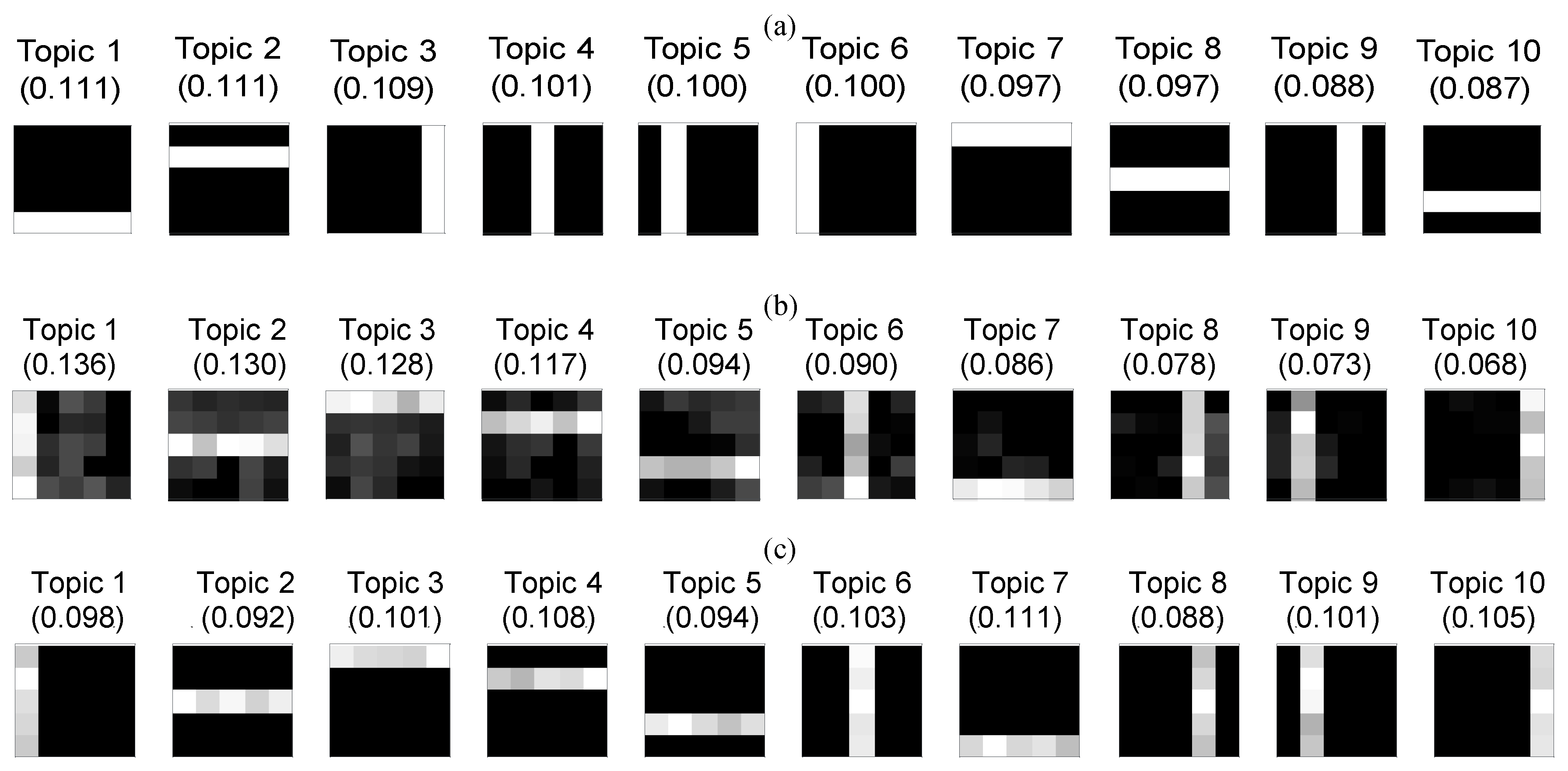
Information generated by the analyses including the: (a) ground truth used to generate low-level data; (b) LDA model; (c) ERT model.
Figure 8.
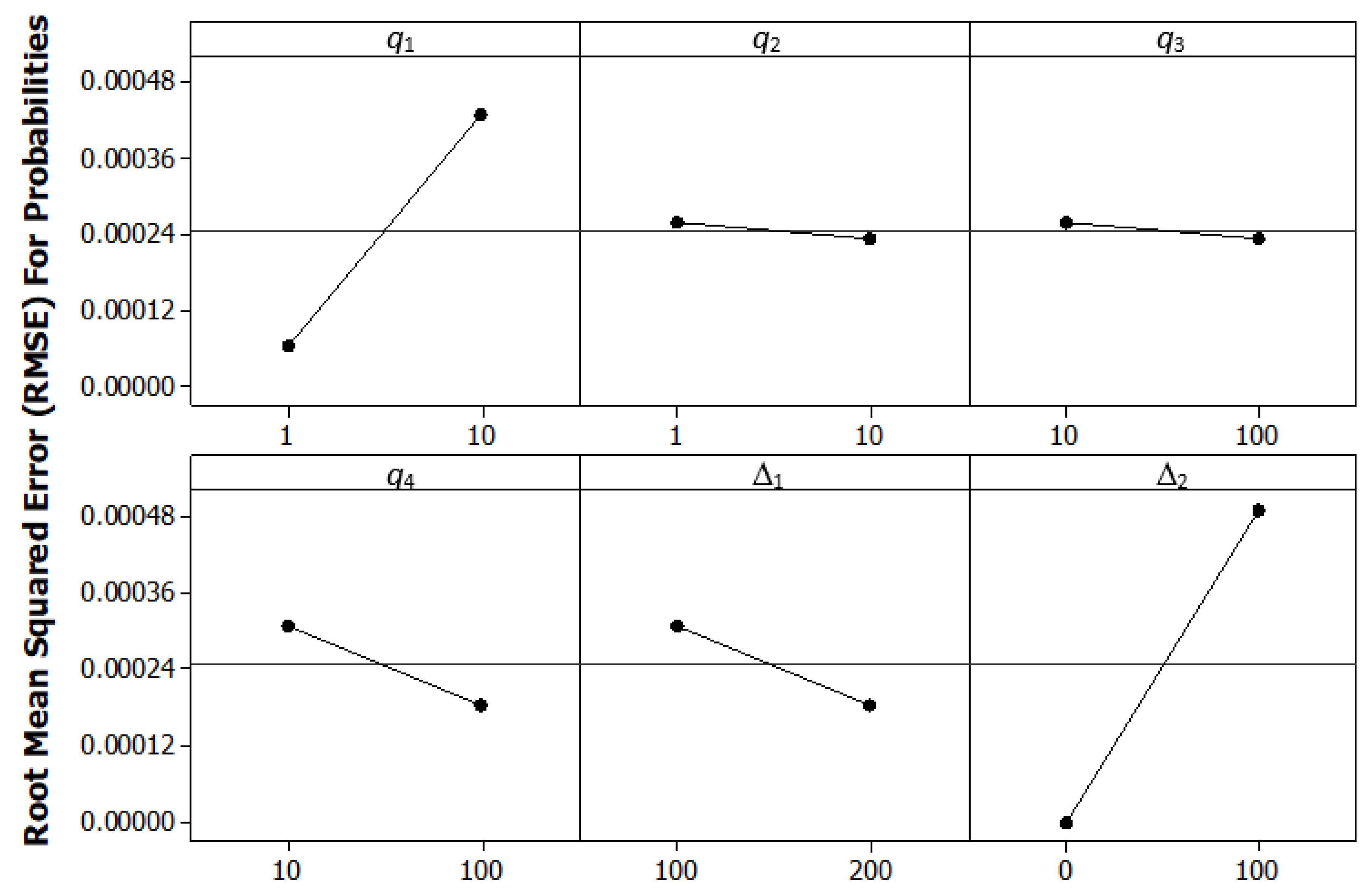
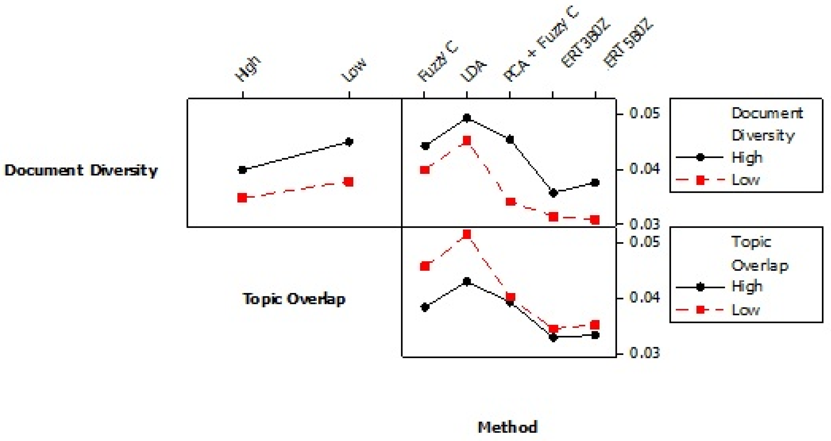
Interaction plot for topic definition minimum average root mean squares (MARMS).
Figure 9.
(a) Ground truth used to generate low-level data; (b) LDA model; (c) ERT model.
Figure 10.
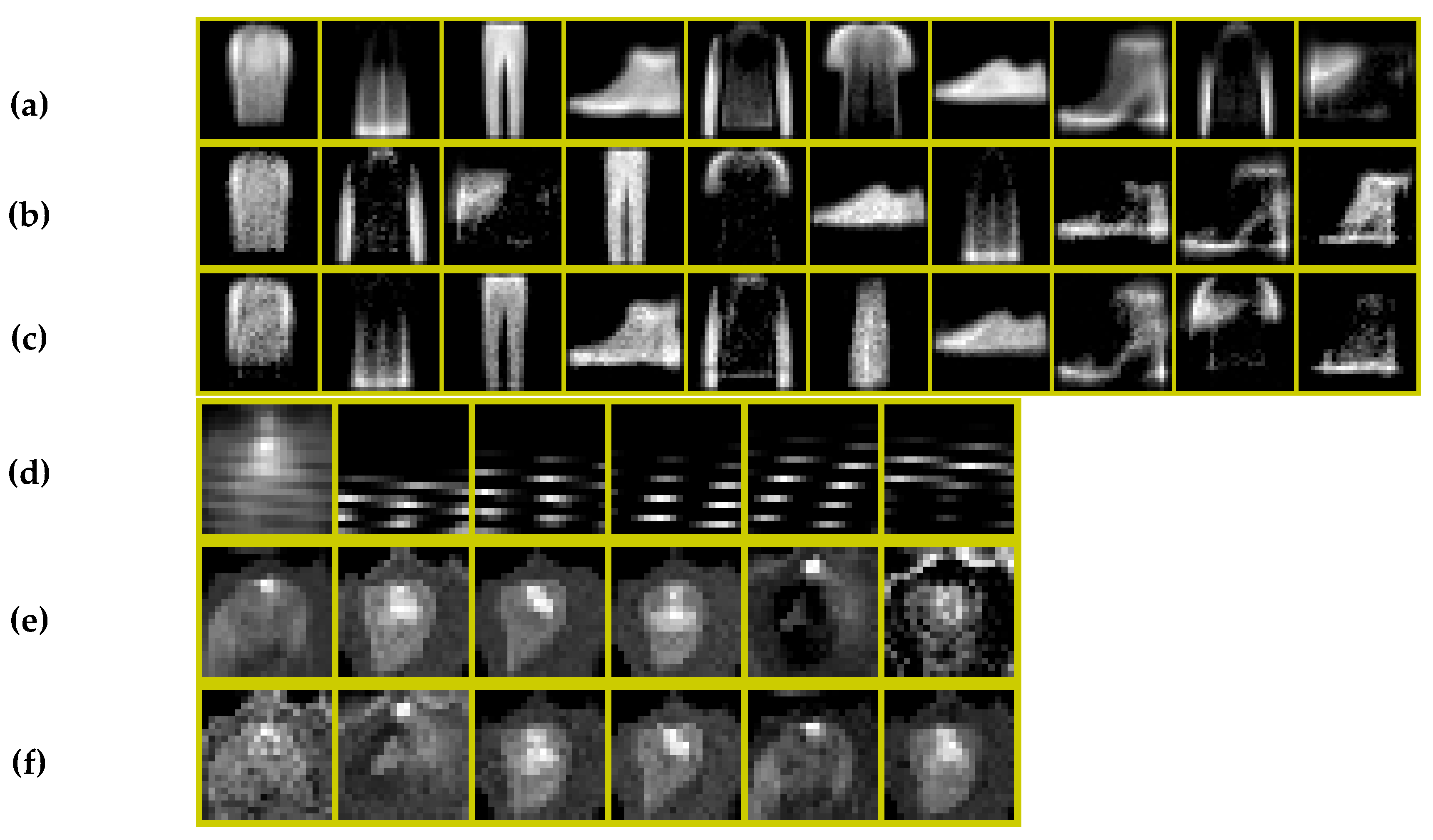
Fashion data (a) LDA topics with 10,000 images, (b) LDA topics with 1000 images, (c) ERT model with 1000 images and Tungsten Inert Gas (TIG) data (d) LDA topics with 10,000 images, (e) LDA topics with 1000 images, (f) ERT model with 1000 images.
Figure 11.
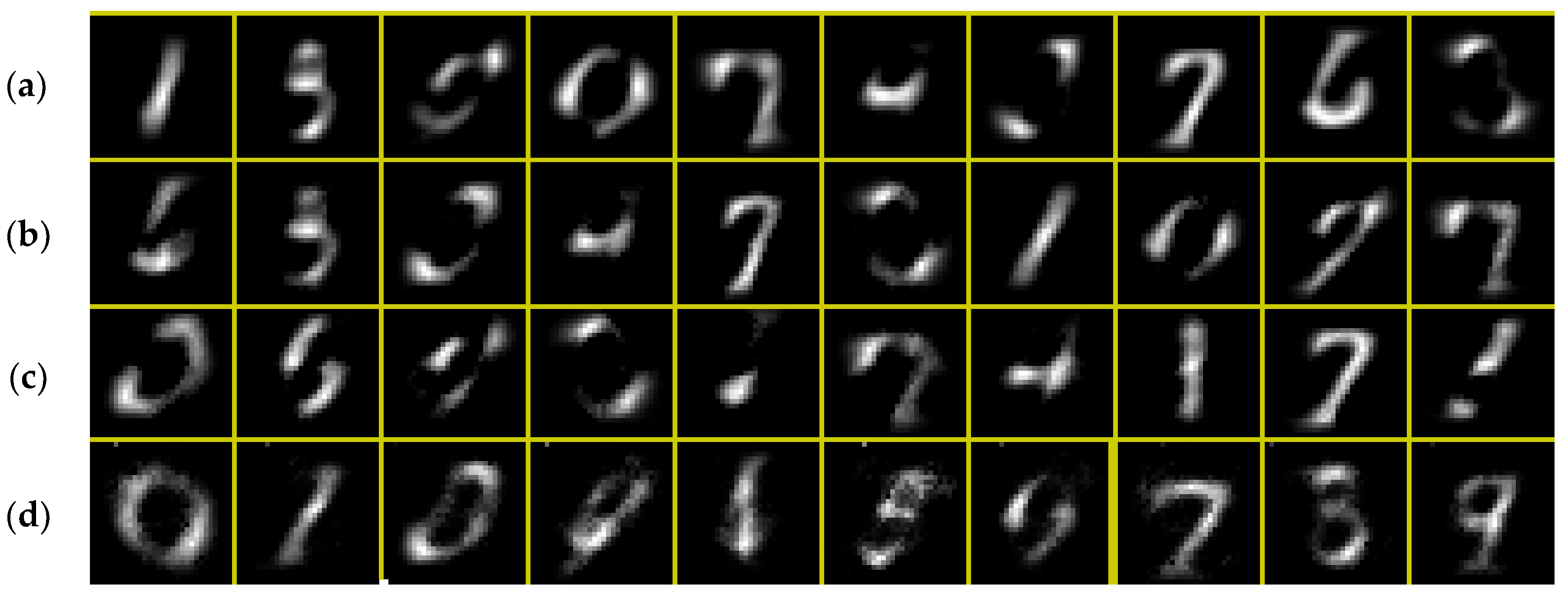
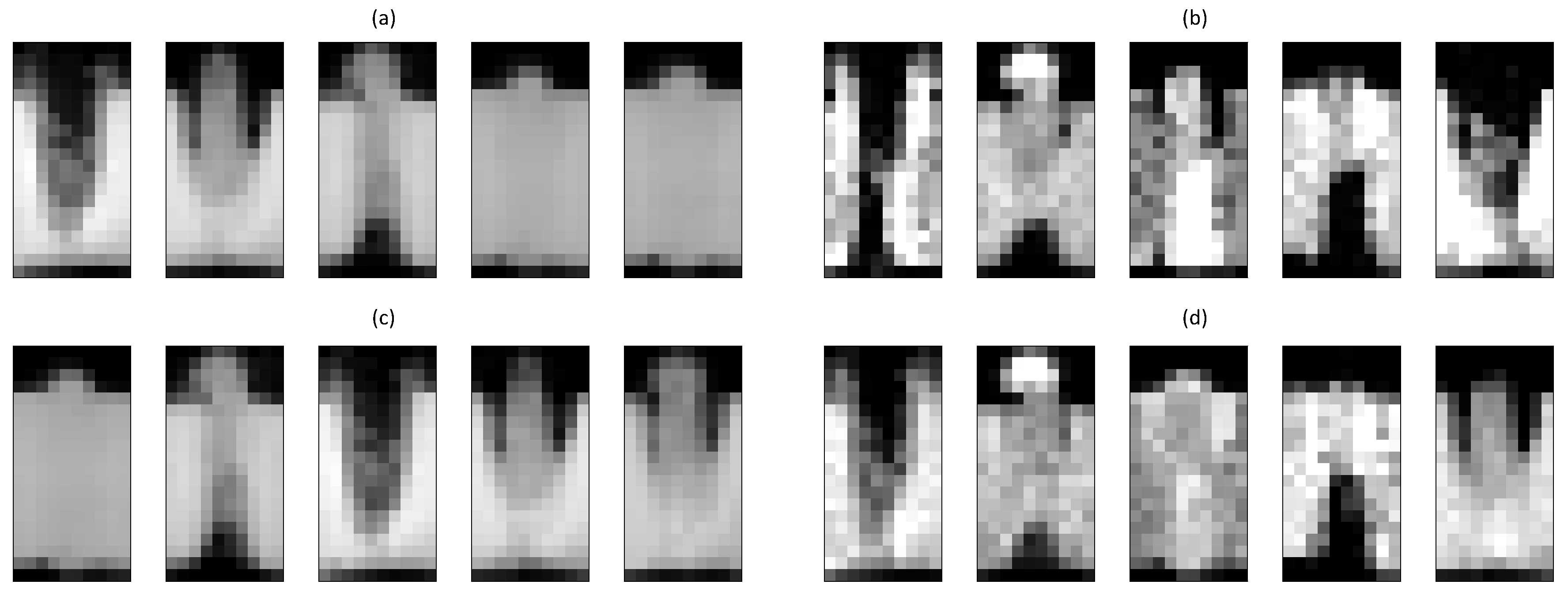
Alternative methods applied to the laser welding problem: (a) fuzzy c clustering, (b) LDA, (c) Principal Component Analysis (PCA) + fuzzy c methods and (d) ERT model topic definitions.
Table 1.
(a) Data for the first low-level image; (b) 25 high-level data points with zaps with one million (M) effective trials and boosts.
| (a) |
| Source 1 |
| 1 | 1 | 1 | 1 | 1 | 1 | 1 | 1 | 3 | 3 |
| 3 | 3 | 3 | 6 | 6 | 6 | 6 | 6 | 6 | 6 |
| 7 | 7 | 7 | 7 | 7 | 7 | 7 | 7 | 7 | 7 |
| 7 | 7 | 7 | 7 | 7 | 8 | 8 | 8 | 8 | 8 |
| 8 | 8 | 10 | 11 | 13 | 13 | 13 | 13 | 13 | 13 |
| 13 | 13 | 13 | 13 | 13 | 13 | 13 | 14 | 15 | 16 |
| 16 | 16 | 16 | 16 | 16 | 16 | 16 | 17 | 17 | 17 |
| 17 | 17 | 17 | 17 | 17 | 17 | 17 | 17 | 18 | 18 |
| 18 | 18 | 18 | 18 | 18 | 20 | 21 | 21 | 21 | 21 |
| 21 | 21 | 21 | 21 | 23 | 23 | 23 | 23 | 23 | 23 |
| (b) |
| Topic | Word (c) | Trials (N) | x |
| 1 | 13 | 1M | 0 |
| 1 | 3 | 1M | 0 |
| 1 | 8 | 1M | 0 |
| 1 | 18 | 1M | 0 |
| 1 | 23 | 1M | 0 |
| 2 | 1 | 1M | 0 |
| 2 | 6 | 1M | 0 |
| 2 | 16 | 1M | 0 |
| 2 | 21 | 1M | 0 |
| 2 | 7 | 1M | 0 |
| 2 | 17 | 1M | 0 |
| 3 | 10 | 2 | 2 |
| 3 | 15 | 2 | 2 |
| 3 | 20 | 2 | 2 |
| 3 | 1 | 1M | 0 |
| 3 | 6 | 1M | 0 |
| 3 | 7 | 1M | 0 |
| 3 | 16 | 1M | 0 |
| 3 | 17 | 1M | 0 |
| 3 | 21 | 1M | 0 |
| 3 | 13 | 1M | 0 |
| 3 | 3 | 1M | 0 |
| 3 | 8 | 1M | 0 |
| 3 | 18 | 1M | 0 |
| 3 | 23 | 1M | 0 |
Table 2.
Kullback–Leibler (KL) distances from: (a) sampling (S) to LDA topics; (b) sampling to ERT topics.
| (a) |
| True | LDA1 | LDA2 | LDA3 | M. | Distance |
| True1 | 5.8401 | 6.3563 | 6.0461 | 1 | 5.8401 |
| True2 | 10.4052 | 9.9058 | 10.0556 | 2 | 9.9058 |
| True3 | 16.0514 | 16.0815 | 16.5708 | 3 | 16.5708 |
| (b) |
| True | ERT1 | ERT2 | ERT3 | M | Distance |
| True1 | 0.1480 | 25.6169 | 25.6613 | 1 | 0.1480 |
| True2 | 25.9283 | 1.4619 | 26.3251 | 2 | 1.4619 |
| True3 | 19.9218 | 15.5279 | 0.3864 | 3 | 0.3864 |
Table 3.
The 200 high-level data points for the bar numerical example. This shows many zaps in the topic definitions.
| # | t | c | N | x | # | t | c | N | x | # | t | c | N | x | # | t | c | N | x |
|---|
| 1 | 1 | 6 | 1M | 0 | 51 | 3 | 14 | 1M | 0 | 101 | 6 | 1 | 1M | 0 | 151 | 8 | 11 | 1M | 0 |
| 2 | 1 | 7 | 1M | 0 | 52 | 3 | 15 | 1M | 0 | 102 | 6 | 2 | 1M | 0 | 152 | 8 | 12 | 1M | 0 |
| 3 | 1 | 8 | 1M | 0 | 53 | 3 | 17 | 1M | 0 | 103 | 6 | 3 | 1M | 0 | 153 | 8 | 13 | 1M | 0 |
| 4 | 1 | 9 | 1M | 0 | 54 | 3 | 18 | 1M | 0 | 104 | 6 | 4 | 1M | 0 | 154 | 8 | 14 | 1M | 0 |
| 5 | 1 | 10 | 1M | 0 | 55 | 3 | 19 | 1M | 0 | 105 | 6 | 5 | 1M | 0 | 155 | 8 | 15 | 1M | 0 |
| 6 | 1 | 11 | 1M | 0 | 56 | 3 | 20 | 1M | 0 | 106 | 6 | 6 | 1M | 0 | 156 | 8 | 21 | 1M | 0 |
| 7 | 1 | 12 | 1M | 0 | 57 | 3 | 22 | 1M | 0 | 107 | 6 | 7 | 1M | 0 | 157 | 8 | 22 | 1M | 0 |
| 8 | 1 | 13 | 1M | 0 | 58 | 3 | 23 | 1M | 0 | 108 | 6 | 8 | 1M | 0 | 158 | 8 | 23 | 1M | 0 |
| 9 | 1 | 14 | 1M | 0 | 59 | 3 | 24 | 1M | 0 | 109 | 6 | 9 | 1M | 0 | 159 | 8 | 24 | 1M | 0 |
| 10 | 1 | 15 | 1M | 0 | 60 | 3 | 25 | 1M | 0 | 110 | 6 | 10 | 1M | 0 | 160 | 8 | 25 | 1M | 0 |
| 11 | 1 | 16 | 1M | 0 | 61 | 4 | 1 | 1M | 0 | 111 | 6 | 16 | 1M | 0 | 161 | 9 | 1 | 1M | 0 |
| 12 | 1 | 17 | 1M | 0 | 62 | 4 | 3 | 1M | 0 | 112 | 6 | 17 | 1M | 0 | 162 | 9 | 2 | 1M | 0 |
| 13 | 1 | 18 | 1M | 0 | 63 | 4 | 4 | 1M | 0 | 113 | 6 | 18 | 1M | 0 | 163 | 9 | 3 | 1M | 0 |
| 14 | 1 | 19 | 1M | 0 | 64 | 4 | 5 | 1M | 0 | 114 | 6 | 19 | 1M | 0 | 164 | 9 | 4 | 1M | 0 |
| 15 | 1 | 20 | 1M | 0 | 65 | 4 | 6 | 1M | 0 | 115 | 6 | 20 | 1M | 0 | 165 | 9 | 5 | 1M | 0 |
| 16 | 1 | 21 | 1M | 0 | 66 | 4 | 8 | 1M | 0 | 116 | 6 | 21 | 1M | 0 | 166 | 9 | 11 | 1M | 0 |
| 17 | 1 | 22 | 1M | 0 | 67 | 4 | 9 | 1M | 0 | 117 | 6 | 22 | 1M | 0 | 167 | 9 | 12 | 1M | 0 |
| 18 | 1 | 23 | 1M | 0 | 68 | 4 | 10 | 1M | 0 | 118 | 6 | 23 | 1M | 0 | 168 | 9 | 13 | 1M | 0 |
| 19 | 1 | 24 | 1M | 0 | 69 | 4 | 11 | 1M | 0 | 119 | 6 | 24 | 1M | 0 | 169 | 9 | 14 | 1M | 0 |
| 20 | 1 | 25 | 1M | 0 | 70 | 4 | 13 | 1M | 0 | 120 | 6 | 25 | 1M | 0 | 170 | 9 | 15 | 1M | 0 |
| 21 | 2 | 1 | 1M | 0 | 71 | 4 | 14 | 1M | 0 | 121 | 7 | 1 | 1M | 0 | 171 | 9 | 16 | 1M | 0 |
| 22 | 2 | 2 | 1M | 0 | 72 | 4 | 15 | 1M | 0 | 122 | 7 | 2 | 1M | 0 | 172 | 9 | 17 | 1M | 0 |
| 23 | 2 | 4 | 1M | 0 | 73 | 4 | 16 | 1M | 0 | 123 | 7 | 3 | 1M | 0 | 173 | 9 | 18 | 1M | 0 |
| 24 | 2 | 5 | 1M | 0 | 74 | 4 | 18 | 1M | 0 | 124 | 7 | 4 | 1M | 0 | 174 | 9 | 19 | 1M | 0 |
| 25 | 2 | 6 | 1M | 0 | 75 | 4 | 19 | 1M | 0 | 125 | 7 | 6 | 1M | 0 | 175 | 9 | 20 | 1M | 0 |
| 26 | 2 | 7 | 1M | 0 | 76 | 4 | 20 | 1M | 0 | 126 | 7 | 7 | 1M | 0 | 176 | 9 | 21 | 1M | 0 |
| 27 | 2 | 9 | 1M | 0 | 77 | 4 | 21 | 1M | 0 | 127 | 7 | 8 | 1M | 0 | 177 | 9 | 22 | 1M | 0 |
| 28 | 2 | 10 | 1M | 0 | 78 | 4 | 23 | 1M | 0 | 128 | 7 | 9 | 1M | 0 | 178 | 9 | 23 | 1M | 0 |
| 29 | 2 | 11 | 1M | 0 | 79 | 4 | 24 | 1M | 0 | 129 | 7 | 11 | 1M | 0 | 179 | 9 | 24 | 1M | 0 |
| 30 | 2 | 12 | 1M | 0 | 80 | 4 | 25 | 1M | 0 | 130 | 7 | 12 | 1M | 0 | 180 | 9 | 25 | 1M | 0 |
| 31 | 2 | 14 | 1M | 0 | 81 | 5 | 1 | 1M | 0 | 131 | 7 | 13 | 1M | 0 | 181 | 10 | 1 | 1M | 0 |
| 32 | 2 | 15 | 1M | 0 | 82 | 5 | 2 | 1M | 0 | 132 | 7 | 14 | 1M | 0 | 182 | 10 | 2 | 1M | 0 |
| 33 | 2 | 16 | 1M | 0 | 83 | 5 | 3 | 1M | 0 | 133 | 7 | 16 | 1M | 0 | 183 | 10 | 3 | 1M | 0 |
| 34 | 2 | 17 | 1M | 0 | 84 | 5 | 5 | 1M | 0 | 134 | 7 | 17 | 1M | 0 | 184 | 10 | 4 | 1M | 0 |
| 35 | 2 | 19 | 1M | 0 | 85 | 5 | 6 | 1M | 0 | 135 | 7 | 18 | 1M | 0 | 185 | 10 | 5 | 1M | 0 |
| 36 | 2 | 20 | 1M | 0 | 86 | 5 | 7 | 1M | 0 | 136 | 7 | 19 | 1M | 0 | 186 | 10 | 6 | 1M | 0 |
| 37 | 2 | 21 | 1M | 0 | 87 | 5 | 8 | 1M | 0 | 137 | 7 | 21 | 1M | 0 | 187 | 10 | 7 | 1M | 0 |
| 38 | 2 | 22 | 1M | 0 | 88 | 5 | 10 | 1M | 0 | 138 | 7 | 22 | 1M | 0 | 188 | 10 | 8 | 1M | 0 |
| 39 | 2 | 24 | 1M | 0 | 89 | 5 | 11 | 1M | 0 | 139 | 7 | 23 | 1M | 0 | 189 | 10 | 9 | 1M | 0 |
| 40 | 2 | 25 | 1M | 0 | 90 | 5 | 12 | 1M | 0 | 140 | 7 | 24 | 1M | 0 | 190 | 10 | 10 | 1M | 0 |
| 41 | 3 | 2 | 1M | 0 | 91 | 5 | 13 | 1M | 0 | 141 | 8 | 1 | 1M | 0 | 191 | 10 | 11 | 1M | 0 |
| 42 | 3 | 3 | 1M | 0 | 92 | 5 | 15 | 1M | 0 | 142 | 8 | 2 | 1M | 0 | 192 | 10 | 12 | 1M | 0 |
| 43 | 3 | 4 | 1M | 0 | 93 | 5 | 16 | 1M | 0 | 143 | 8 | 3 | 1M | 0 | 193 | 10 | 13 | 1M | 0 |
| 44 | 3 | 5 | 1M | 0 | 94 | 5 | 17 | 1M | 0 | 144 | 8 | 4 | 1M | 0 | 194 | 10 | 14 | 1M | 0 |
| 45 | 3 | 7 | 1M | 0 | 95 | 5 | 18 | 1M | 0 | 145 | 8 | 5 | 1M | 0 | 195 | 10 | 15 | 1M | 0 |
| 46 | 3 | 8 | 1M | 0 | 96 | 5 | 20 | 1M | 0 | 146 | 8 | 6 | 1M | 0 | 196 | 10 | 16 | 1M | 0 |
| 47 | 3 | 9 | 1M | 0 | 97 | 5 | 21 | 1M | 0 | 147 | 8 | 7 | 1M | 0 | 197 | 10 | 17 | 1M | 0 |
| 48 | 3 | 10 | 1M | 0 | 98 | 5 | 22 | 1M | 0 | 148 | 8 | 8 | 1M | 0 | 198 | 10 | 18 | 1M | 0 |
| 49 | 3 | 12 | 1M | 0 | 99 | 5 | 23 | 1M | 0 | 149 | 8 | 9 | 1M | 0 | 199 | 10 | 19 | 1M | 0 |
| 50 | 3 | 13 | 1M | 0 | 100 | 5 | 25 | 1M | 0 | 150 | 8 | 10 | 1M | 0 | 200 | 10 | 20 | 1M | 0 |
Table 4.
KL distances from: (a) sampling (S) to LDA topics; (b) sampling to ERT (SM) topics.
| (a) |
| True | LDA1 | LDA2 | LDA3 | LDA4 | LDA5 | LDA6 | LDA7 | LDA8 | LDA9 | LDA10 | M. | SKLD |
| True1 | 11.735 | 17.543 | 17.072 | 18.732 | 16.917 | 11.487 | 1.625 | 15.089 | 17.305 | 14.733 | 7 | 1.625 |
| True2 | 15.367 | 13.628 | 14.362 | 4.175 | 15.719 | 16.352 | 20.028 | 13.045 | 13.831 | 15.554 | 4 | 4.175 |
| True3 | 19.184 | 13.224 | 14.740 | 11.620 | 10.874 | 16.358 | 16.846 | 13.438 | 20.525 | 0.826 | 10 | 0.826 |
| True4 | 13.354 | 15.048 | 12.553 | 14.818 | 15.444 | 4.040 | 15.638 | 18.329 | 17.717 | 18.037 | 6 | 4.040 |
| True5 | 15.957 | 14.095 | 11.527 | 13.543 | 15.472 | 17.619 | 13.433 | 18.227 | 2.181 | 18.782 | 9 | 2.181 |
| True6 | 5.810 | 12.624 | 12.989 | 15.081 | 15.195 | 16.413 | 15.618 | 18.551 | 16.902 | 20.962 | 1 | 5.810 |
| True7 | 14.073 | 14.527 | 5.976 | 16.036 | 13.825 | 12.995 | 20.513 | 16.851 | 17.520 | 14.544 | 3 | 5.976 |
| True8 | 12.944 | 5.982 | 14.020 | 15.453 | 18.161 | 17.094 | 18.289 | 14.326 | 14.613 | 15.857 | 2 | 5.982 |
| True9 | 15.137 | 12.078 | 14.484 | 16.773 | 12.799 | 18.294 | 15.991 | 3.767 | 19.836 | 18.757 | 8 | 3.767 |
| True10 | 15.323 | 15.389 | 14.863 | 17.439 | 5.164 | 14.795 | 17.071 | 13.000 | 13.891 | 16.676 | 5 | 5.164 |
| (b) |
| True | SM1 | SMS2 | SM3 | SM4 | SM5 | SM6 | SM7 | SM8 | SM9 | SM10 | M. | SKLD |
| True1 | 20.984 | 25.917 | 25.917 | 25.920 | 25.918 | 20.823 | 0.006 | 21.026 | 21.052 | 20.731 | 7 | 0.006 |
| True2 | 20.198 | 25.917 | 25.917 | 0.009 | 25.918 | 20.775 | 25.919 | 20.776 | 20.219 | 20.947 | 4 | 0.009 |
| True3 | 25.918 | 20.668 | 20.324 | 20.161 | 20.768 | 25.916 | 21.174 | 25.919 | 25.922 | 0.003 | 10 | 0.003 |
| True4 | 25.918 | 20.571 | 20.924 | 20.577 | 20.845 | 0.001 | 20.817 | 25.919 | 25.922 | 25.917 | 6 | 0.001 |
| True5 | 25.918 | 20.931 | 20.875 | 21.237 | 20.296 | 25.916 | 20.230 | 25.919 | 0.013 | 25.917 | 9 | 0.013 |
| True6 | 0.005 | 20.422 | 20.595 | 20.989 | 20.604 | 25.916 | 20.817 | 25.919 | 25.922 | 25.917 | 1 | 0.005 |
| True7 | 20.968 | 25.917 | 0.004 | 25.920 | 25.918 | 20.610 | 25.919 | 21.026 | 20.707 | 20.862 | 3 | 0.004 |
| True8 | 20.710 | 0.004 | 25.917 | 25.920 | 25.918 | 20.548 | 25.919 | 20.124 | 20.354 | 20.354 | 2 | 0.004 |
| True9 | 25.918 | 21.081 | 20.956 | 20.726 | 21.165 | 25.916 | 20.643 | 0.007 | 25.922 | 25.917 | 8 | 0.007 |
| True10 | 20.818 | 25.917 | 25.917 | 25.920 | 0.006 | 20.909 | 25.919 | 20.730 | 21.368 | 20.777 | 5 | 0.006 |
Table 5.
The 198 high-level data points for the laser welding example.
| # | t | c | N | x | # | t | c | N | x | # | t | c | N | x | # | t | c | N | x |
|---|
| 1 | 1 | 58 | 20 | 20 | 51 | 2 | 106 | 20 | 20 | 101 | 3 | 148 | 20 | 20 | 151 | 4 | 111 | 20 | 20 |
| 2 | 1 | 59 | 20 | 20 | 52 | 2 | 107 | 20 | 20 | 102 | 3 | 149 | 20 | 20 | 152 | 4 | 131 | 20 | 20 |
| 3 | 1 | 66 | 10 | 10 | 53 | 2 | 108 | 20 | 20 | 103 | 3 | 154 | 20 | 20 | 153 | 4 | 185 | 20 | 20 |
| 4 | 1 | 67 | 10 | 10 | 54 | 2 | 109 | 20 | 20 | 104 | 3 | 156 | 20 | 20 | 154 | 4 | 169 | 20 | 20 |
| 5 | 1 | 68 | 10 | 10 | 55 | 2 | 110 | 20 | 20 | 105 | 3 | 165 | 20 | 20 | 155 | 4 | 171 | 20 | 20 |
| 6 | 1 | 69 | 10 | 10 | 56 | 2 | 126 | 20 | 20 | 106 | 3 | 166 | 20 | 20 | 156 | 4 | 177 | 20 | 20 |
| 7 | 1 | 70 | 10 | 10 | 57 | 2 | 127 | 20 | 20 | 107 | 3 | 167 | 20 | 20 | 157 | 4 | 178 | 20 | 20 |
| 8 | 1 | 71 | 10 | 10 | 58 | 2 | 128 | 20 | 20 | 108 | 3 | 168 | 20 | 20 | 158 | 4 | 186 | 20 | 20 |
| 9 | 1 | 72 | 10 | 10 | 59 | 2 | 129 | 20 | 20 | 109 | 3 | 170 | 20 | 20 | 159 | 4 | 187 | 20 | 20 |
| 10 | 1 | 73 | 20 | 20 | 60 | 2 | 130 | 20 | 20 | 110 | 3 | 174 | 20 | 20 | 160 | 4 | 188 | 20 | 20 |
| 11 | 1 | 74 | 20 | 20 | 61 | 2 | 131 | 20 | 20 | 111 | 3 | 175 | 20 | 20 | 161 | 5 | 64 | 20 | 20 |
| 12 | 1 | 75 | 20 | 20 | 62 | 2 | 59 | 20 | 20 | 112 | 3 | 176 | 20 | 20 | 162 | 5 | 65 | 20 | 20 |
| 13 | 1 | 76 | 20 | 20 | 63 | 2 | 77 | 20 | 20 | 113 | 3 | 190 | 20 | 20 | 163 | 5 | 66 | 20 | 20 |
| 14 | 1 | 77 | 20 | 20 | 64 | 2 | 78 | 20 | 20 | 114 | 3 | 192 | 20 | 20 | 164 | 5 | 69 | 20 | 20 |
| 15 | 1 | 78 | 20 | 20 | 65 | 2 | 79 | 20 | 20 | 115 | 4 | 44 | 1M | 0 | 165 | 5 | 84 | 20 | 20 |
| 16 | 1 | 79 | 20 | 20 | 66 | 2 | 96 | 20 | 20 | 116 | 4 | 84 | 10 | 10 | 166 | 5 | 85 | 20 | 20 |
| 17 | 1 | 87 | 10 | 10 | 67 | 2 | 97 | 20 | 20 | 117 | 4 | 104 | 10 | 10 | 167 | 5 | 86 | 20 | 20 |
| 18 | 1 | 88 | 10 | 10 | 68 | 2 | 98 | 20 | 20 | 118 | 4 | 5 | 20 | 20 | 168 | 5 | 87 | 20 | 20 |
| 19 | 1 | 89 | 10 | 10 | 69 | 2 | 99 | 20 | 20 | 119 | 4 | 11 | 20 | 20 | 169 | 5 | 88 | 20 | 20 |
| 20 | 1 | 90 | 10 | 10 | 70 | 2 | 116 | 20 | 20 | 120 | 4 | 14 | 20 | 20 | 170 | 5 | 89 | 20 | 20 |
| 21 | 1 | 91 | 10 | 10 | 71 | 2 | 117 | 20 | 20 | 121 | 4 | 15 | 20 | 20 | 171 | 5 | 90 | 20 | 20 |
| 22 | 1 | 92 | 20 | 20 | 72 | 2 | 118 | 20 | 20 | 122 | 4 | 16 | 20 | 20 | 172 | 5 | 92 | 20 | 20 |
| 23 | 1 | 93 | 20 | 20 | 73 | 2 | 119 | 20 | 20 | 123 | 4 | 17 | 20 | 20 | 173 | 5 | 93 | 20 | 20 |
| 24 | 1 | 94 | 20 | 20 | 74 | 2 | 137 | 20 | 20 | 124 | 4 | 18 | 20 | 20 | 174 | 5 | 104 | 20 | 20 |
| 25 | 1 | 95 | 20 | 20 | 75 | 2 | 138 | 20 | 20 | 125 | 4 | 30 | 20 | 20 | 175 | 5 | 105 | 20 | 20 |
| 26 | 1 | 96 | 20 | 20 | 76 | 2 | 139 | 20 | 20 | 126 | 4 | 32 | 20 | 20 | 176 | 5 | 106 | 20 | 20 |
| 27 | 1 | 97 | 20 | 20 | 77 | 2 | 43 | 1M | 0 | 127 | 4 | 33 | 20 | 20 | 177 | 5 | 107 | 20 | 20 |
| 28 | 1 | 98 | 20 | 20 | 78 | 2 | 81 | 1M | 0 | 128 | 4 | 35 | 20 | 20 | 178 | 5 | 108 | 20 | 20 |
| 29 | 1 | 99 | 20 | 20 | 79 | 3 | 83 | 1M | 0 | 129 | 4 | 36 | 20 | 20 | 179 | 5 | 109 | 20 | 20 |
| 30 | 1 | 199 | 30 | 30 | 80 | 3 | 103 | 1M | 0 | 130 | 4 | 37 | 20 | 20 | 180 | 5 | 110 | 20 | 20 |
| 31 | 1 | 22 | 1M | 0 | 81 | 3 | 6 | 20 | 20 | 131 | 4 | 38 | 20 | 20 | 181 | 5 | 111 | 20 | 20 |
| 32 | 1 | 162 | 1M | 0 | 82 | 3 | 10 | 20 | 20 | 132 | 4 | 50 | 20 | 20 | 182 | 5 | 112 | 20 | 20 |
| 33 | 1 | 185 | 10 | 10 | 83 | 3 | 12 | 20 | 20 | 133 | 4 | 48 | 20 | 20 | 183 | 5 | 113 | 20 | 20 |
| 34 | 2 | 46 | 10 | 10 | 84 | 3 | 13 | 20 | 20 | 134 | 4 | 53 | 20 | 20 | 184 | 5 | 114 | 20 | 20 |
| 35 | 2 | 148 | 20 | 20 | 85 | 3 | 34 | 20 | 20 | 135 | 4 | 54 | 20 | 20 | 185 | 5 | 124 | 20 | 20 |
| 36 | 2 | 46 | 20 | 20 | 86 | 3 | 26 | 20 | 20 | 136 | 4 | 56 | 20 | 20 | 186 | 5 | 125 | 20 | 20 |
| 37 | 2 | 47 | 20 | 20 | 87 | 3 | 45 | 20 | 20 | 137 | 4 | 65 | 20 | 20 | 187 | 5 | 126 | 20 | 20 |
| 38 | 2 | 48 | 20 | 20 | 88 | 3 | 46 | 20 | 20 | 138 | 4 | 66 | 20 | 20 | 188 | 5 | 127 | 20 | 20 |
| 39 | 2 | 49 | 20 | 20 | 89 | 3 | 47 | 20 | 20 | 139 | 4 | 69 | 20 | 20 | 189 | 5 | 128 | 20 | 20 |
| 40 | 2 | 50 | 20 | 20 | 90 | 3 | 49 | 20 | 20 | 140 | 4 | 71 | 20 | 20 | 190 | 5 | 129 | 20 | 20 |
| 41 | 2 | 66 | 20 | 20 | 91 | 3 | 59 | 20 | 20 | 141 | 4 | 72 | 20 | 20 | 191 | 5 | 130 | 20 | 20 |
| 42 | 2 | 67 | 20 | 20 | 92 | 3 | 125 | 20 | 20 | 142 | 4 | 73 | 20 | 20 | 192 | 5 | 131 | 20 | 20 |
| 43 | 2 | 68 | 20 | 20 | 93 | 3 | 126 | 20 | 20 | 143 | 4 | 74 | 20 | 20 | 193 | 5 | 132 | 20 | 20 |
| 44 | 2 | 69 | 20 | 20 | 94 | 3 | 127 | 20 | 20 | 144 | 4 | 75 | 20 | 20 | 194 | 5 | 133 | 20 | 20 |
| 45 | 2 | 70 | 20 | 20 | 95 | 3 | 128 | 20 | 20 | 145 | 4 | 76 | 20 | 20 | 195 | 5 | 134 | 20 | 20 |
| 46 | 2 | 86 | 20 | 20 | 96 | 3 | 129 | 20 | 20 | 146 | 4 | 77 | 20 | 20 | 196 | 5 | 135 | 20 | 20 |
| 47 | 2 | 87 | 20 | 20 | 97 | 3 | 130 | 20 | 20 | 147 | 4 | 78 | 20 | 20 | 197 | 5 | 158 | 20 | 20 |
| 48 | 2 | 88 | 20 | 20 | 98 | 3 | 145 | 20 | 20 | 148 | 4 | 86 | 20 | 20 | 198 | 5 | 159 | 20 | 20 |
| 49 | 2 | 89 | 20 | 20 | 99 | 3 | 146 | 20 | 20 | 149 | 4 | 87 | 20 | 20 | | | | | |
| 50 | 2 | 90 | 20 | 20 | 100 | 3 | 147 | 20 | 20 | 150 | 4 | 105 | 20 | 20 | | | | | |
Table 6.
Topic assignment probabilities from the ERT for the 20 laser welding images.
| | 1st Topic (Prob.) | 2nd Topic (Prob.) | 3rd Topic (Prob.) | 4th Topic (Prob.) | 5th Topic (Prob.) |
|---|
| source 1 | 5 (0.675) | 2 (0.316) | 1 (0.005) | 3 (0.004) | 4 (0.000) |
| source 2 | 5 (0.904) | 4 (0.093) | 1 (0.002) | 2 (0.001) | 3 (0.000) |
| source 3 | 3 (0.896) | 5 (0.091) | 4 (0.012) | 2 (0.001) | 1 (0.000) |
| source 4 | 3 (0.749) | 5 (0.162) | 4 (0.088) | 1 (0.000) | 2 (0.000) |
| source 5 | 3 (0.648) | 2 (0.166) | 5 (0.106) | 4 (0.080) | 1 (0.000) |
| source 6 | 3 (0.689) | 5 (0.220) | 4 (0.089) | 1 (0.002) | 2 (0.000) |
| source 7 | 5 (0.826) | 2 (0.165) | 4 (0.006) | 1 (0.002) | 3 (0.001) |
| source 8 | 5 (0.747) | 2 (0.252) | 1 (0.001) | 3 (0.000) | 4 (0.000) |
| source 9 | 3 (0.898) | 2 (0.057) | 5 (0.040) | 4 (0.002) | 1 (0.002) |
| source 10 | 3 (0.951) | 4 (0.042) | 5 (0.008) | 1 (0.000) | 2 (0.000) |
| source 11 | 3 (0.685) | 5 (0.210) | 4 (0.101) | 1 (0.004) | 2 (0.000) |
| source 12 | 3 (0.748) | 2 (0.225) | 4 (0.014) | 1 (0.011) | 5 (0.003) |
| source 13 | 4 (0.583) | 2 (0.406) | 3 (0.006) | 5 (0.005) | 1 (0.000) |
| source 14 | 2 (0.735) | 4 (0.258) | 1 (0.005) | 3 (0.001) | 5 (0.001) |
| source 15 | 2 (0.714) | 4 (0.278) | 1 (0.006) | 5 (0.001) | 3 (0.001) |
| source 16 | 3 (0.986) | 4 (0.008) | 5 (0.003) | 1 (0.002) | 2 (0.001) |
| source 17 | 4 (0.803) | 2 (0.197) | 3 (0.000) | 1 (0.000) | 5 (0.000) |
| source 18 | 1 (0.780) | 5 (0.214) | 3 (0.004) | 2 (0.002) | 4 (0.000) |
| source 19 | 1 (0.994) | 4 (0.003) | 3 (0.002) | 5 (0.001) | 2 (0.000) |
| source 20 | 1 (0.521) | 4 (0.478) | 3 (0.001) | 2 (0.000) | 5 (0.000) |
© 2020 by the authors. Licensee MDPI, Basel, Switzerland. This article is an open access article distributed under the terms and conditions of the Creative Commons Attribution (CC BY) license (http://creativecommons.org/licenses/by/4.0/).
