Article

Visual Exploration of Large Multidimensional Data Using Parallel Coordinates on Big Data Infrastructure

LaBRI, UMR 5800, Université de Bordeaux, 351, cours de la Libération F-33405 Talence cedex, France
*
Author to whom correspondence should be addressed.
Informatics 2017, 4(3), 21; https://doi.org/10.3390/informatics4030021
Submission received: 31 May 2017 / Revised: 30 June 2017 / Accepted: 10 July 2017 / Published: 12 July 2017
(This article belongs to the Special Issue Scalable Interactive Visualization)

Abstract

:
The increase of data collection in various domains calls for an adaptation of methods of visualization to tackle magnitudes exceeding the number of available pixels on screens and challenging interactivity. This growth of datasets size has been supported by the advent of accessible and scalable storage and computing infrastructure. Similarly, visualization systems need perceptual and interactive scalability. We present a complete system, complying with the constraints of aforesaid environment, for visual exploration of large multidimensional data with parallel coordinates. Perceptual scalability is addressed with data abstraction while interactions rely on server-side data-intensive computation and hardware-accelerated rendering on the client-side. The system employs a hybrid computing method to accommodate pre-computing time or space constraints and achieves responsiveness for main parallel coordinates plot interaction tools on billions of records.

1. Introduction

Recent years have seen a striking increase in the amount of collected and generated data. For instance, in web analytics, visitors’ behavior is analyzed to the event-level to improve services and marketing strategies. Naturally, such amounts bring about new challenges for storing, querying and analyzing these ever-growing datasets. Among other approaches, information visualization enables the exploration and understanding of complex data without prior knowledge of the patterns and trends to identify. However, traditional information visualization systems are not fitted for large-scale data exploration and have to be adapted to tackle the new challenges that arise from the surge of dataset sizes. The first consequence of this growth is the increase of the time needed to process the data. Another consequence is the separation of the data storage from the visualization client. Often, large data are stored on distant repositories and cannot reasonably be moved since the time (and storage on the destination computer) necessary for such operation is too important to be considered. Finally, the screen space is physically limited by its number of available pixels and large amounts of visual elements either cannot fit or become indistinguishable. Therefore, scalable visualization systems have to address three main challenges: perceptual scalability, interactive scalability and remoteness. Perceptual scalability refers to screen space and user capabilities limitations when depicting large data. Interactive scalability encompasses the latencies incurred by processing and querying large data for interaction. Remoteness corresponds to data processing and visualization being performed at separate locations which induces data transfer. To limit latencies during interaction, the visualization system has to be designed with this major bottleneck in mind.
Various visualization techniques are dedicated to quantitative multivariate data: scatterplot matrices [1], hyperboxes [2], star coordinates [3], Andrew curves [4] and parallel coordinates [5] are well-known examples. In the parallel coordinates technique, all dimensions of the multidimensional data are represented as parallel axes and each record as a polyline. A record’s polyline intersects each axis at its corresponding dimensional value (see Figure 1a). The strength of this plot is that it offers an overview of the multidimensional data since each dimension is displayed uniformly. However, the patterns revealed by a plot strongly depend on the arbitrary placement of its axes [6]. For this reason, interactive axis reordering and flipping are necessary to grasp all pairwise relations between dimensions. Brushing is another fundamental interaction as it makes possible to select and enhance a subset of multidimensional items on top of the original view, following a focus+context approach. For hundred of thousands of items, traditional line-based parallel coordinate plot induces substantial visual clutter [7] (see Figure 1b) and interaction latencies. Several approaches have been proposed to deal with these challenges, ranging from using visual enhancement [8], via interactive tools [9], to joint representations of data subsets [10]. These techniques, either data-driven or screen-based, successfully handle up to millions of records. However, some may conceal patterns and most techniques are not adapted for remote visualization constraints.
Adapting parallel coordinates for the interactive visualization of large and remote data requires schemes to bound the size of the transferred data from the storing location to the visualization point. One solution lies in using a form of data reduction and representing an abstract version of the data, of a bounded size, regardless of the original dataset size. A second requirement is having a similar adaptability (or scalability) in the processing capabilities of the system, relative to the workload induced by interactive manipulation like brushing. This can be achieved using horizontal scalable systems which seamlessly parallelize processing over a network of computing and storage units where data is replicated and partitioned. While vertical scalability denotes the addition of extra resources on the same unit (e.g., expanding storage or adding a CPU), horizontal scalability is the concept of using multiple units as a single one. Systems that scale horizontally can theoretically satisfy any increase in processing demand with the expansion of their network of units.
The main contribution of this paper is a scalable system suited for interactive visual exploration of large multidimensional data with an abstract parallel coordinates representation. The novelty of this approach is the horizontal scalability of the system which relies on distributed processing in the form of pre-computation and on-demand computation, and on data aggregation. The use of distributed processing using scalable components for interaction allows performance to be tailored seamlessly to achieve responsiveness. The use of data aggregation provides boundaries for: (1) storage for pre-computed data, (2) data transfer between a distributed storage and computing infrastructure and a rendering client and (3) displayed items.
In the following section, we present two topics of related work: perceptual scalability on parallel coordinates and large-scale visualization systems. Next, in Section 3, we describe the work-flow as well as the main components of our system. We then describe the abstract parallel coordinates representation implemented (Section 4) and discuss interactive scalability for panning, zooming, axis rearrangement and selection in Section 5. In Section 6 we demonstrate the effectiveness of the abstract visualization and in Section 7, the system performances. Finally, we present the conclusions and discuss the possible future works.

2. Related Work

On line-based parallel coordinate representations, each multidimensional data item is depicted with a polyline and the multiplication of such polylines produces a rapid increase in the usage of pixels as the dataset gets larger. Such consumption of pixels is not practical for large datasets: the plot rapidly becomes overcrowded as polylines cross and overlap. Moreover, rendering and interaction complexity generally depend on the dataset size which requires fast data querying techniques to ensure responsiveness for large datasets. In this context, we discuss two topics of related work. First, existing methods for effectively avoiding clutter and over-plot in parallel coordinates and secondly, previous works on scalable visualization systems for parallel-coordinate representations and others.

2.1. Overcoming Clutter in Parallel Coordinates

A first approach to deal with clutter in parallel coordinates lies in visual enhancement for clarifying dense areas and facilitating pattern recognition. This can be accomplished using density-based methods [8,12,13] or curves instead of lines [14,15,16]. However, such methods do not scale as they are, since they require to draw every item. According to Ellis and Dix [17], clutter reduction techniques that directly meet the scalable criteria are sampling, filtering, and clustering. In Ellis and Dix [9], sampling is applied locally, with an interactive lens, to unclutter the plot. Similarly, filtering is used by numerous prior works [18,19,20] as an interactive and user-controlled tool. Johansson and Cooper [21] introduced a screen-space measure to filter items while preserving significant features with better results than data-space measures. Using sampling or filtering for data reduction has the advantage of keeping a consistent visual representation of items, regardless of the chosen level of detail. However, these approaches have limitations as a general methods to avoid clutter. For example, filtering often requires prerequisite knowledge of the data, otherwise meaningful structures or outliers may be unintentionally hidden.
Clustering the data is another possible approach adopted in many previous works. Cluster-based enhancement on traditional representations facilitates identification of multidimensional groups of items by using visual cues such as color, opacity or bundling. For example, in Johansson et al. [22] transfer functions are applied independently to high-precision textures generated for each computed cluster. Luo et al. [23] use curved bundles which both help to trace lines trough axes and facilitate the identification of groups. Representing aggregates instead of their covered subset of items/polylines further reduces visual clutter and may speed up the rendering. Aggregates have been represented using statistical metrics [24], envelopes or bounding-boxes [5,10,18,25]. Fua et al. [18] render both multidimensional clusters as polygons and mean values as dense lines and McDonnell and Mueller [10] draw bundled envelopes. This approach has been generalized to hierarchical clustering [18,26] to support multiscale exploration.
As stated by Palmas et al. [27], multidimensional data reduction (sampling or clustering) enhances global trends to the cost of potentially concealing pairwise relationships between dimensions. Novotny and Hauser [28] propose a hybrid solution which separates the rendering of outliers from the rest. On the one hand, data are clustered using a binning clustering technique and two-dimensional bins are represented using parallelograms. On the other hand, outliers are rendered using polylines. Doing so, in-between axis information is not degraded and clusters are sharper due to outliers having been primarily filtered out. The bundled parallel coordinates presented by Palmas et al. [27] uses one-dimensional clustering which improves visual continuity on axes compared to [28]. One-dimensional clustering creates meta-link between axis aggregates, similar to Kosara et al. [29]’s Parallel Sets which deals with nominal data inducing natural groups on axes. Matchmaker [30] presents comparable weighted and curved meta-links between axes, however, the clustering technique employed is applied on groups of dimensions which relates to the specific case of inherent groupings between dimensions.
Most of these techniques efficiently handle up to dozens of thousands of items for rendering. However, they do not scale to millions or billions of items. To the best of our knowledge, it is mainly due to their computational and memory costs with standard computers. This challenge is precisely the scope of this paper.

2.2. Scalable Visualization Systems
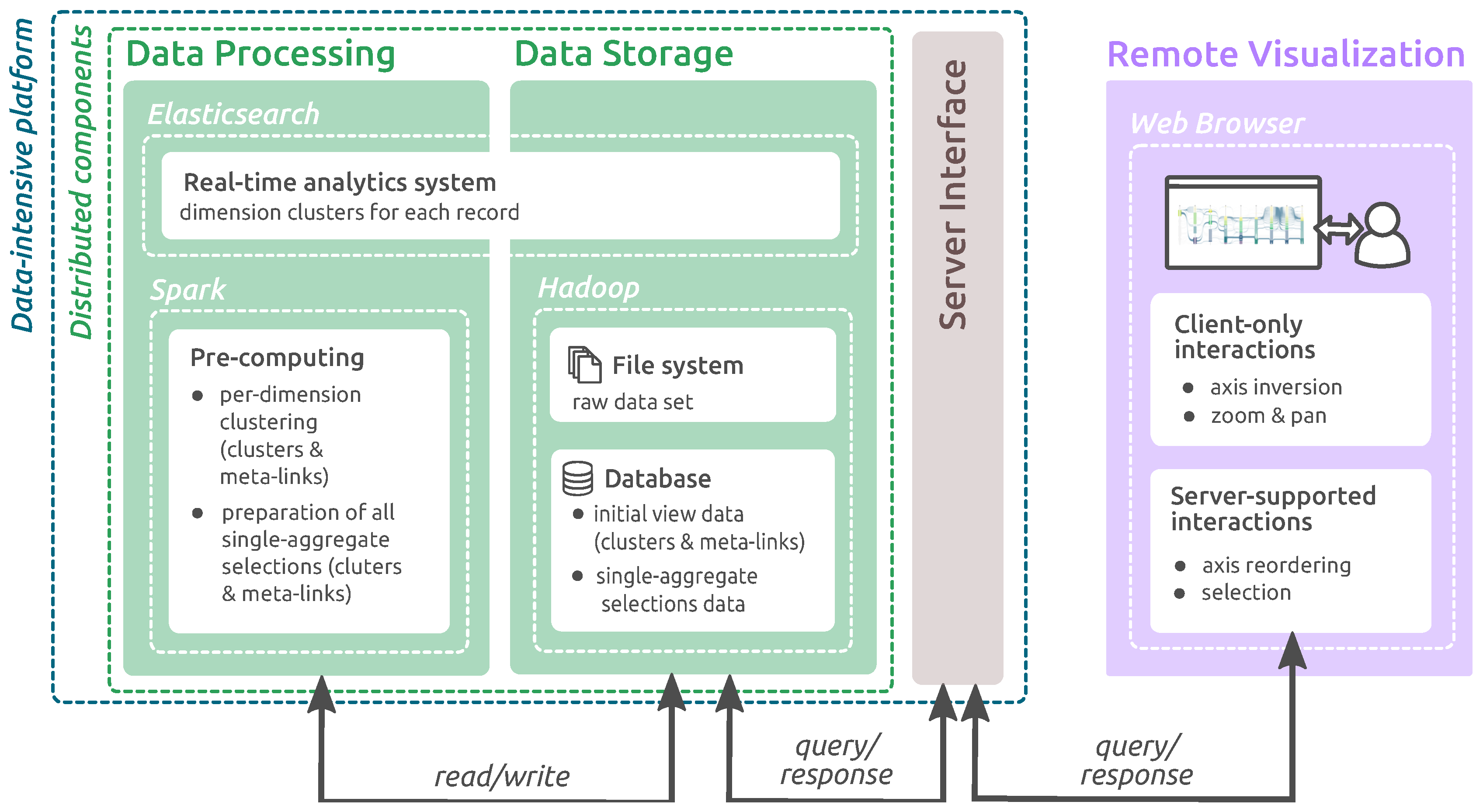
When data becomes too massive to fit inside a computer’s memory, input/output communication with slower, external or remote, memory and data-processing time create a substantial bottleneck for interactive visualization. Solutions arise from hardware upgrades (vertical scalability) with parallel processing, distributed methods (horizontal scalability) and other strategies (e.g., out-of-core methods, data abstraction, tailored indexing).
Hardware acceleration of modern GPU is now frequently used [18,22,25,31] to render millions of items in real-time. Parallel processing can also serve data processing with dedicated multi-core computing units [32], distributed systems of servers running on commodity hardware [33,34] or multi-threading [35]. Other mechanisms to enable interactivity at large scale include pre-computing [31,33] and pre-fetching, incremental approaches, and data abstraction with multi-resolution representations [18,33,36]. For instance, Rübel et al. [32] and Perrot et al. [33] propose systems associating several of these solutions to scale interactive representations (respectively parallel coordinate and heatmaps) to extremely large datasets. Rübel et al. [32] present a system combining the multi-resolution binning technique of Novotny and Hauser [28] and FastBit [37], an index/query tool, on a supercomputer. Perrot et al. [33] use Canopy clustering for multilevel heatmaps computed over a distributed infrastructure, most similar to our setting.
Ideally, a visual exploration system should support interaction following the user’s flow of thoughts [38] i.e., should operate in less than one second. Generally, bringing interactivity on modest systems operating on large data is a trade-off between pre-computation, approximate computation [39] and the cost of the hardware used. For instance, Rübel et al. [32] use a supercomputer system to achieve 0.15 s response time for tracing 500 items, over a dataset of almost 200 million items, with 100 computing units. In this paper, we target common-hardware and use an infrastructure where the distributed storage is leveraged for computation. Compared to supercomputers, these infrastructures do not offer as efficient communication between units and generally less computing power. Nevertheless, they are much more accessible and affordable and quite common nowadays in various domains (e.g., web analytics). To address data transfer, we use data reduction in the form of aggregation, with per-dimension clustering, as described in the following section.

3. System Overview

Our system lies on two major parts, (1) an abstract representation which addresses the transfer bottleneck and the perceptual scalability, (2) all interactions requiring the full data to be computed occur in a distributed manner on a data-intensive back-end platform. This way, two levers are available for supporting increasingly large data sets and/or improving interactivity: the level of detail which, among other things, impacts the client-server transfer time, and the computing and storage resources of the back-end by expanding the network of computing units. The main components of our system are laid out on Figure 2: the back-end is composed of distributed components that store and process the data, as well as a server acting as its interface. The client renders and animates the representations and interacts with the server for completing interactions that involve the full data. First, we describe the overall work-flow that takes place on the data-intensive platform. Then, we motivate and precise the abstraction used.

3.1. Distributed Processing Work-Flow

The platform is used for hosting the raw data and computing abstract representations for different states of the visualization: corresponding to the initial view or resulting from user interactions. The different types of queries performed by the client are: display of a dataset for a given axis ordering and brushing data given a set of selected aggregates. The back-end computes a per-dimension clustering of the raw dataset and the aggregates (clusters and meta-links) corresponding to those two types of query. While the aggregates formed from the full data are always computed in a preparatory step, the one formed from subsets (used in brushing), result from both beforehand and on-demand computed data depending on the query type.
The pre-computing step (see Figure 2) encompasses computing an abstraction of the raw data and the results of several queries which are inserted into the distributed database. The abstraction, resulting from per-dimension clustering, is subsequently indexed into the real-time analytics system in the form of n vectors (one for each record) where each components gives the cluster identifier of the corresponding dimension. Queries are forwarded by the server, depending on their type, to the prepared data storage or to the analytics system for on-demand filtering and aggregation. On the latter system, cost is related to the number of records involved whereas in the former it is constant.

3.2. Bounding Data Transfer

We use per-dimension clustering as an aggregation strategy. The number of produced clusters for each dimension (called resolution parameter k) together with the number of dimensions (noted d), determines the number of rendered elements. Consequently, controlling and tuning this resolution parameter or degree of reduction conditions the transfer data size, the client memory footprint and the amount of displayed items. Moreover, rendering and interactions that can be performed on the abstract data have complexity independent of the underlying data set size, meeting the interactive scalability criterion. Thus, the performances of the abstract visualization become solely dependent on k and the number of displayed dimension rather than the actual number of records.
Clustering algorithms group items based on a measure of similarity which creates a simplified version of the original data, ideally with meaningful groups (clusters). No omnipotent clustering algorithm is suited for all type of data. Various algorithm have been used in state-of-the-art techniques (Fua et al. [18] uses Birch algorithm, Van Long and Linsen [26] uses a grid-based algorithm, Palmas et al. [27] uses kernel density estimation). In this article, any clustering algorithm can be chosen as long as it produces a strict partitioning of the interval of dimension values, i.e., all resulting clusters should form non-overlapping intervals. Among the various possibilities (k-means [40], DBSCAN [41], binning or adaptive binning as used in [28]). In the performance evaluation of our system, we used Perrot et al. [33]’s Canopy clustering since our prerequisites were similar: a small number of passes over the data to limit processing time and an efficient distributed implementation.
For a fixed resolution parameter k, defined prior to pre-computation, we expect a maximum of k clusters per-dimension. An abstraction is composed of those d · k clusters and the meta-links induces between axes, amounting to at most k 2 between each pair of axes. Clusters have, as properties, their extrema values, their cardinality/weight and a distribution of their values, meta-links have their size. As a result, the total number of items to be transferred between server and client is effectively bounded by k · d + k 2 · d , where d is the number of displayed dimensions. Additionally, exchanges between the server and the two different storage components benefit from the same bound. Indeed, in both cases the transferred data have been aggregated beforehand.

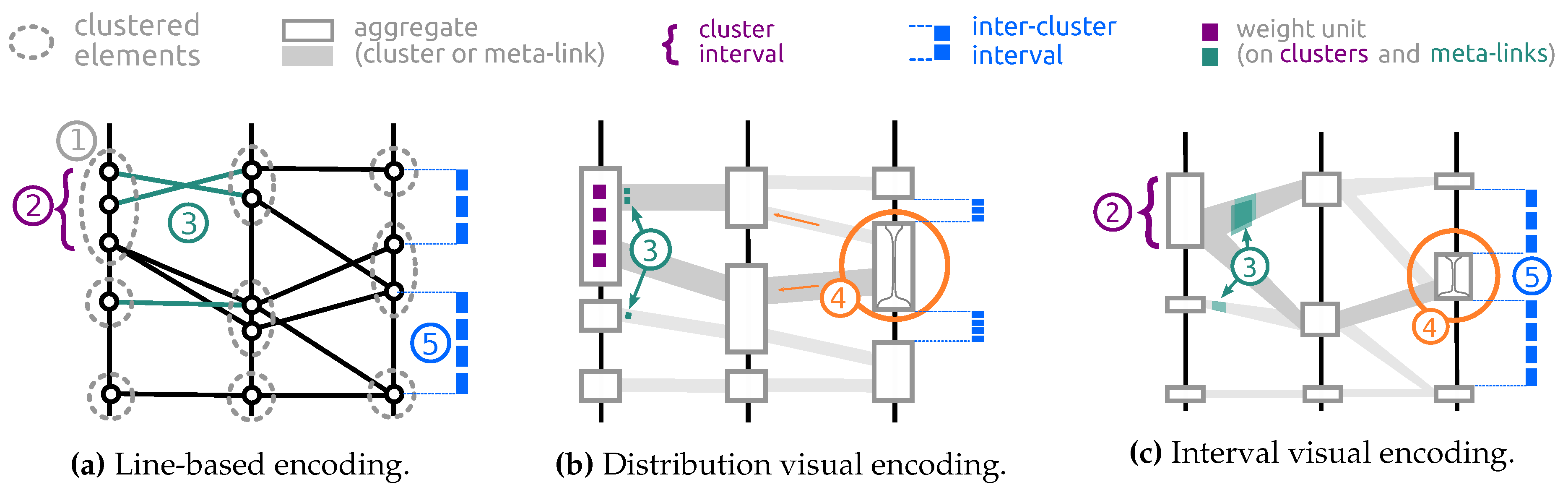
4. Abstract Parallel Coordinates Design

In this section, we focus on the abstract representation design. Similar to Palmas et al. [27], we cluster values on each dimension and bundles lines between pairs of clusters into meta-links. We explored visual metaphors for both types of aggregates (clusters and meta-links) inspired by Palmas et al. [27] and Kosara et al. [29]’s Parallel Sets while striving to reduce occlusion and retain the general overview. The overall design also resembles Sankey diagrams (e.g., [42]), which are specifically designed to represent flow data.
Our abstract parallel coordinates design uses a distribution visual encoding of clusters. With such encoding, the size of cluster representations depends on the number of elements in the corresponding subset (see Figure 3 and Figure 4b). This approach has been widely used in many visualization techniques for rendering abstract elements (e.g., matrix based diagrams). Using this weight depiction, one can easily find which clusters are the most important for a given dimension and if they are connected to many small clusters or rather to a few large ones. Each cluster of a dimension covers both an interval of values and a subset of records/items, with intervals being non-overlapping as stated in Section 3. Using this visual encoding does not natively provide the information of the interval covered by the subset. To solve this issue, we added an inter-clusters spacing to convey an approximation of their covered interval (see Figure 4b). This way, the relative distance between clusters can be assessed and compared. To provide a better insight of this information we also implement an interval visual encoding similar to Palmas et al. [27]’s representation (see Figure 3 and Figure 4c). These two different encoding strategies reflect the dual interpretation of clusters: either as a sub-space of a dimension or as set of close items. In both case, clusters surfaces are leveraged with the display of a smoothed mirrored histogram providing an overview of the values distribution (see Figure 3). This histogram is computed using 10 regular bins (equal-size intervals) for each cluster, with all bin sizes normalized per axis. For each attribute, the larger the bin is, the closer the histogram is to the edges of the cluster.
Meta-links are two-dimensional aggregates, and as such, bear an analogous encoding to clusters. They are represented as ribbons with the size of the subset they cover mapped to their thickness or ends sizes depending on the encoding. Several methods are used to reduce in-between axes clutter. In the distribution visual encoding, meta-links that end on the same cluster are vertically spaced and sorted to minimize crossings as in [29,30] which highly reduces clutter. In both encodings, meta-links are rendered as Bézier curves thinned down in their middle part. Additionally, color intensity and depth sorting are used to further enhance the largest meta-links.
All these features make possible, analyzing both aggregates (clusters and meta-links), to compare at a dimension scale the sizes, densities, separations and distributions on axes. Additionally, using the interval encoding, the slope of meta-links can be used to draw, to some extent, conclusion on the relationship between neighbouring dimensions. The distribution encoding emphasizes larger groups, and consequently major trends, while also tremendously reducing in-between axes clutter but does not provide the ability to assess relationship between dimensions due to the cluster positioning and meta-link positioning schemes. This illustrates the complementarity of both visual encodings.

5. Enabling Interactivity

With usual parallel coordinates tasks in mind, we first identify a set of interactions adapted to abstract parallel coordinates and complying with data processing and transfer constraints. We expose their pre-computation costs and the corresponding chosen strategy (pre-computing or on-demand processing).

5.1. Tasks & Interactions

Common tasks for parallel coordinates include gaining an overview, evaluating correlation between dimensions, identifying subsets of items presenting similar features, and searching for item with a particular multidimensional profile. Gaining a complete overview of multidimensional data implies being able to see every pairs of dimensions. However, without interaction, the ordering of axes only represents a fraction of all the information the dataset contains (non-contiguous dimension relationships are not represented). Bringing axes side-by-side allows an analysis of the meta-links and eases clusters distribution comparison. Using the interval encoding, it also allows the identification of correlation, recognizable by parallel meta-links between the two considered axes. Various tools exist to perform this operation: axis replacement, swap or move.
In abstract parallel coordinates, the aggregation of close dimension values facilitates the distinction of groups of items exhibiting similar features on a given dimension. Highlighting a subset of items permits tracing them across all dimensions. To find items falling into a specific range of values on different dimension, we implement a single-aggregate selection (see Figure 5a) triggered by click on clusters and meta-links and a compound aggregate selection triggered by axis sliders in a filtering fashion (see Figure 5b). Subset highlighting acts as a brushing interaction where selection only operates on aggregates (both clusters and bi-dimensional aggregates, also called meta-links). A selected subset is represented over meta-links and clusters with a gauge showing the proportion of the selected items they contain (see Figure 5a,b) in the distribution encoding and with color intensity in the interval encoding. Additionally, inner-cluster distributions are updated to reflect the distribution of the selected subset only. Making possible to select a subset and emphasize its distribution on the overall representation to compare and analyze the dataset is the core of the focus+context visualization step. The two following sections will describe the interaction tools implemented to allow these tasks. Other solutions that this work will not cover are the grand tour [43], optimum axis placement, and dimensionality reduction.

5.2. Client-Only Interaction & Parameters

Our system supports various interaction tools to help the user in its exploration. Several rendering parameters can be tweaked to instantly obtain different views as they are handled on the client side solely:
  • Zoom and pan: the most classical interaction tool to explore and navigate within a representation.
  • Axis height: used to tune the aspect ratio of the representation by increasing or reducing the height of the axes.
  • Cluster width: can help the user by emphasizing or reducing the focus on the clusters (and the histogram within).
  • Meta-link thickness: changing the thickness makes possible to emphasize the meta-links between clusters rather than the clusters themselves.
  • Meta-link curvature: curving and bundling the meta-link is often used to reduce the clutter, tuning the degree of curvature makes possible to optimize the clutter reduction and Meta-link visibility.
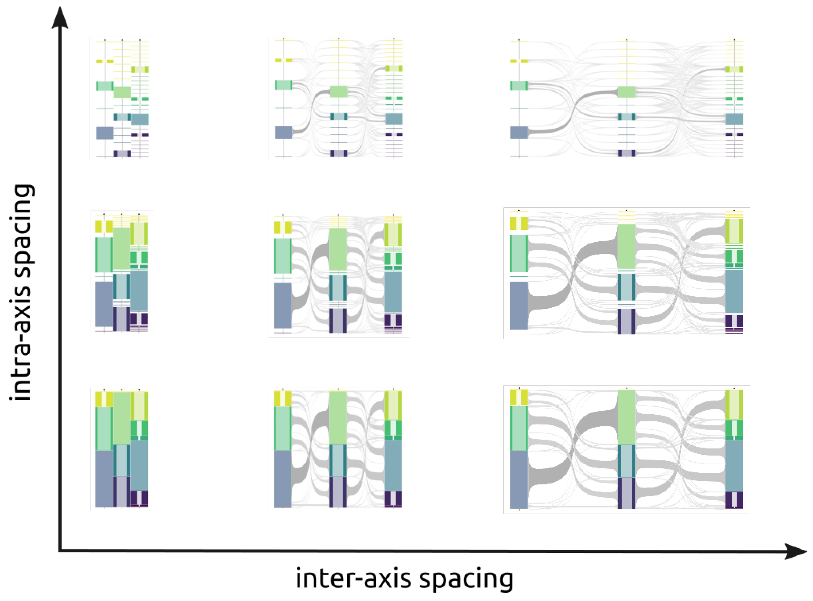
  • Inter-axis spacing: increasing (or reducing) the space between axes makes possible to increase the focus either on clusters or on meta-links and changes the aspect ratio of the representation.
  • Intra-axis spacing: the percentage of empty space allocated to represent the relative distance between clusters (as presented in Section 4) can be reduced at no space (results in displaying a stacked histogram, see Figure 6) or increased to focus on the relative distance between clusters.
  • Axis inversion: inverting an axis may help reducing unnecessary clutter by decreasing the number of crossings.

5.3. Server-Supported Interaction

As the visualization client only stores the necessary data to display the abstracted parallel coordinate view, interactions that need to update the rendered data require for data to be transferred from the server to the client.
  • Axis reordering: the use of this interaction tool is to compensate the main drawback of parallel coordinates: as axes are aligned, comparisons can only be made between pairs of attributes. Furthermore, datasets with a lot of attributes are difficult to read because of the horizontal resolution limit of screens. Moving an axis within the representation implies to update the meta-links between the moved axis and its neighbors (before and after the displacement).
  • Removing or adding axis: Removing an axis is used to reduce the width of the representation by hiding unnecessary axis. As the need for an attribute can change over time and with user needs, each hidden axis can be shown again.
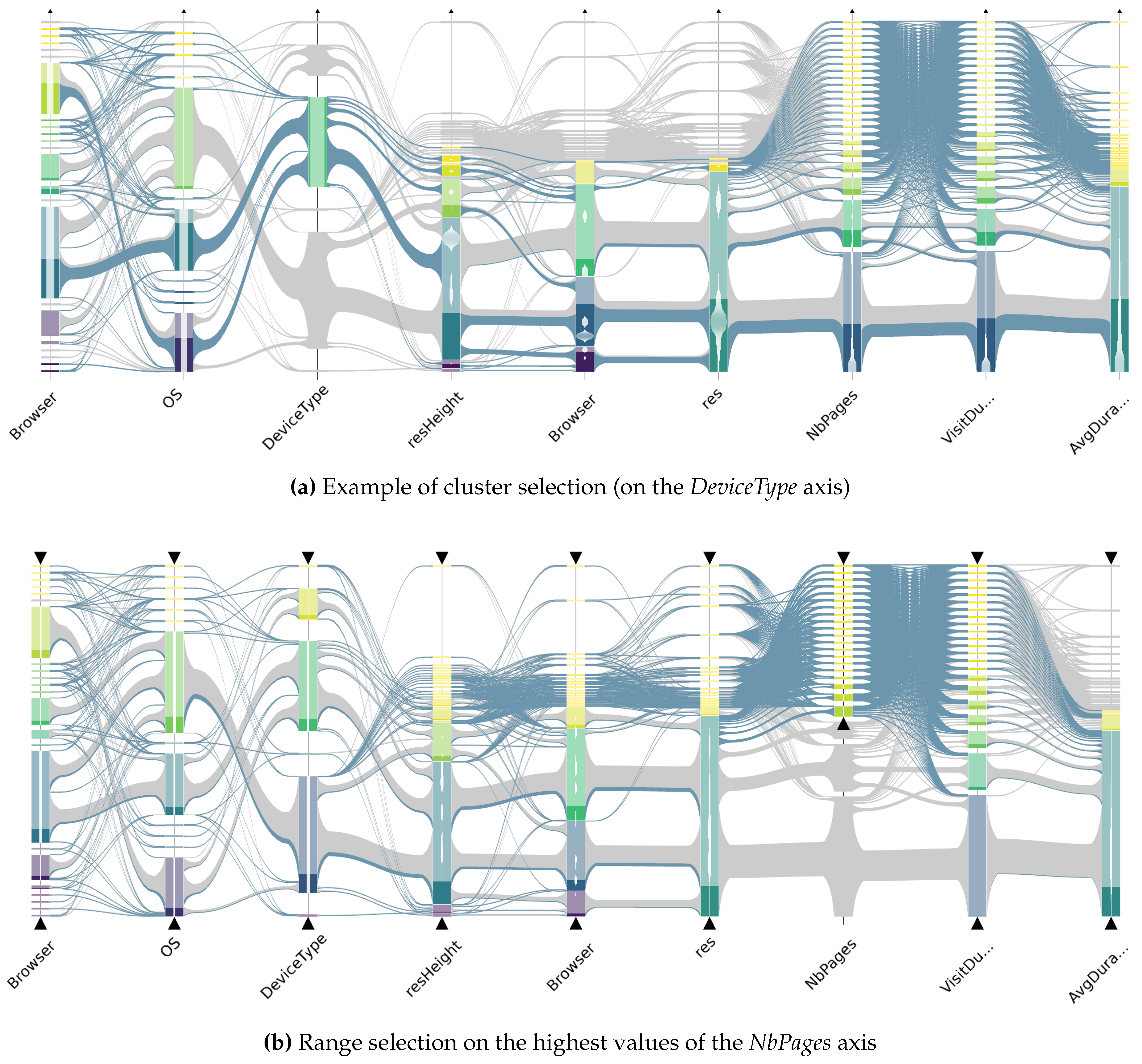
  • Aggregate selection: This interaction allows to bring the focus on aggregates and emphasizes the distribution of the selected subset on the displayed attributes. The total number of meta-links for a given abstracted dataset is always less than k 2 · d 2 . Hence, the maximum number of different single-aggregate selections is k · d + k 2 · d 2 , considering that subset selection can be applied to any cluster or meta-link in any axis ordering. The total number of aggregates to compute for the operation is bounded by k 4 · d 4 . This boundary remains reasonable for moderate k (resolution parameter) and d (number of dimensions) values.
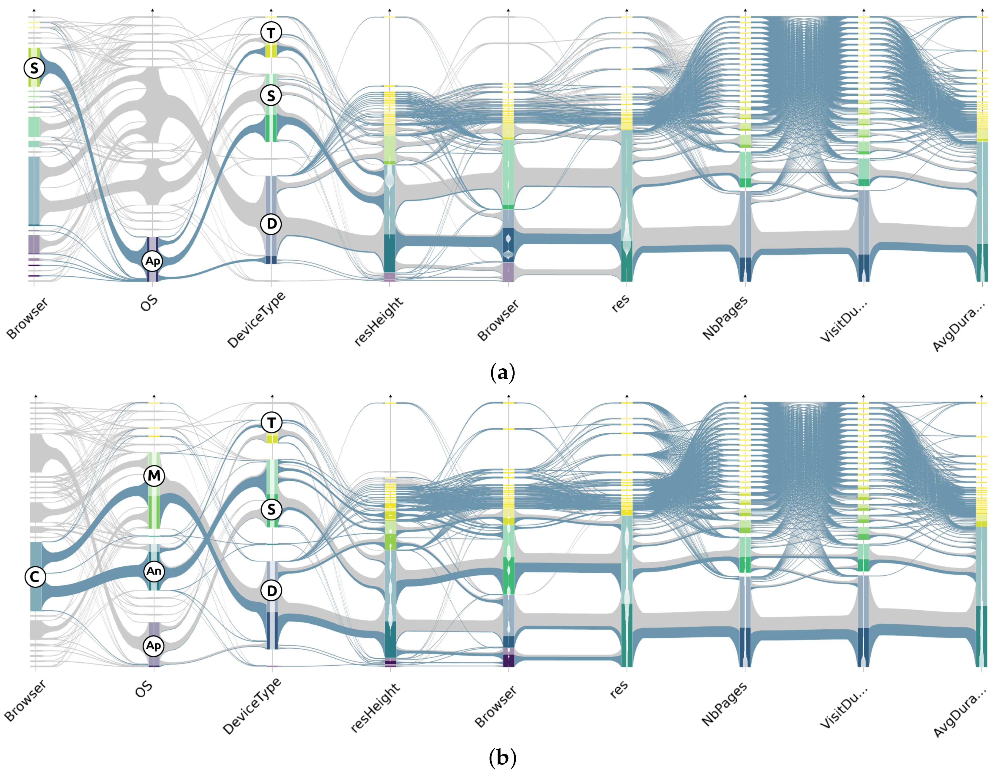
  • Compound selection: This interaction has similar effect as the Aggregate selection (see Figure 5b) but is triggered by axis sliders that define an interval of interest on each dimension and allows the selection of several groups of consecutive clusters on different dimensions at once, corresponding to set operations between aggregates’ subsets. Unlike aggregate selection, these selections cannot be reasonably pre-computed: multiple dimension criteria create a combinatorial explosion of different sub-selections. This is why we handle their computation in real-time.
Tracking individual items could easily be implemented using the on-demand computing scheme. However, this would require an additional medium for choosing and picking the desired item since the visualization technique does not discriminate individual items.

6. Perceptual Scalability

This section presents the effectiveness of the technique described in this article.
Our technique is based on abstract visualization and as such, functions identically regardless of the dataset size, large or not. Indeed, only the chosen resolution parameter influences the representation (see Section 5). On the contrary, traditional line-based technique do not scale visually to large data. Thus, we perform two case-studies: a comparison with traditional parallel coordinate plot using a state-of-the-art dataset (the cars dataset provided in [44] with 400 records) and an exploratory analysis of large data (with 1.6 billions of records).

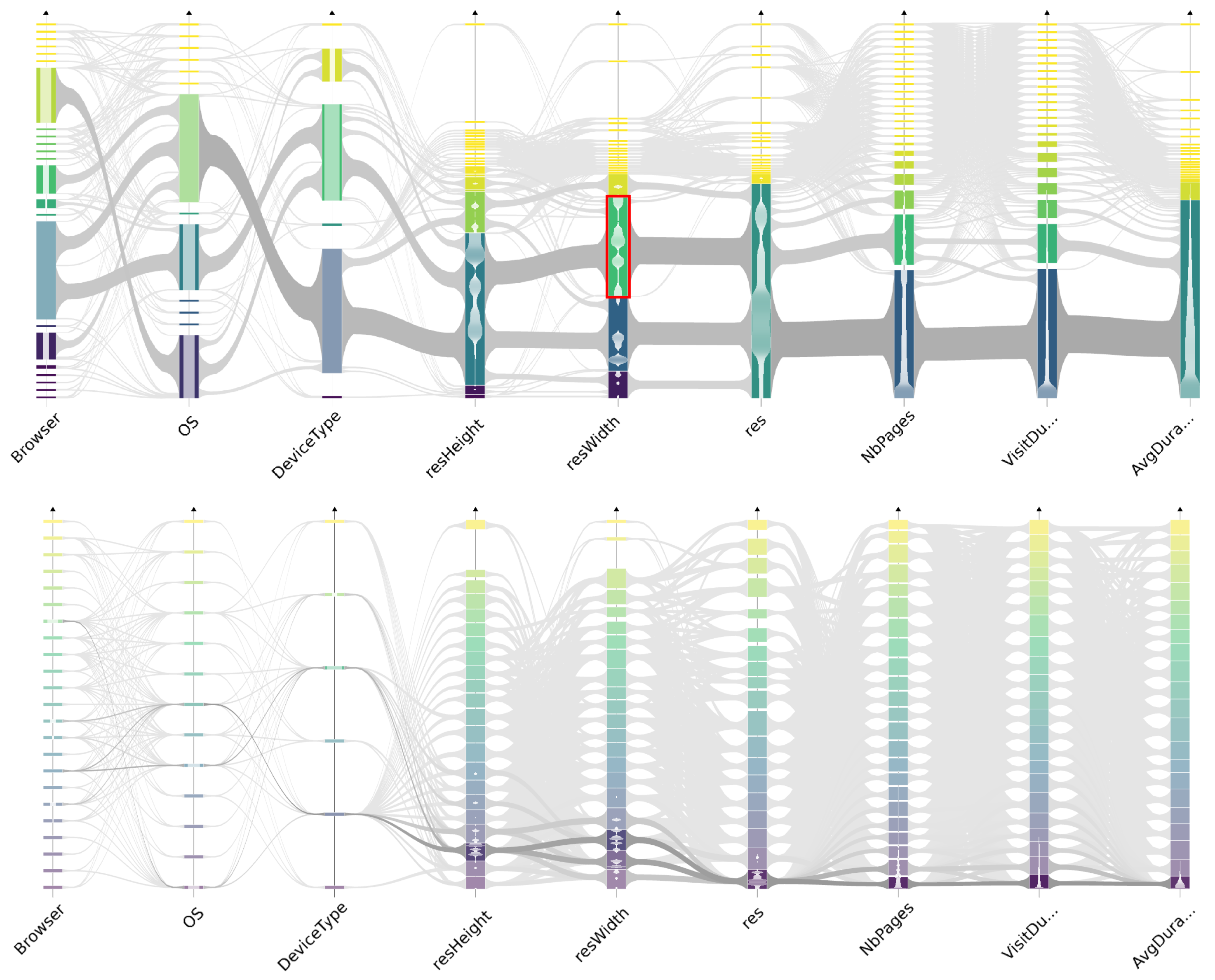
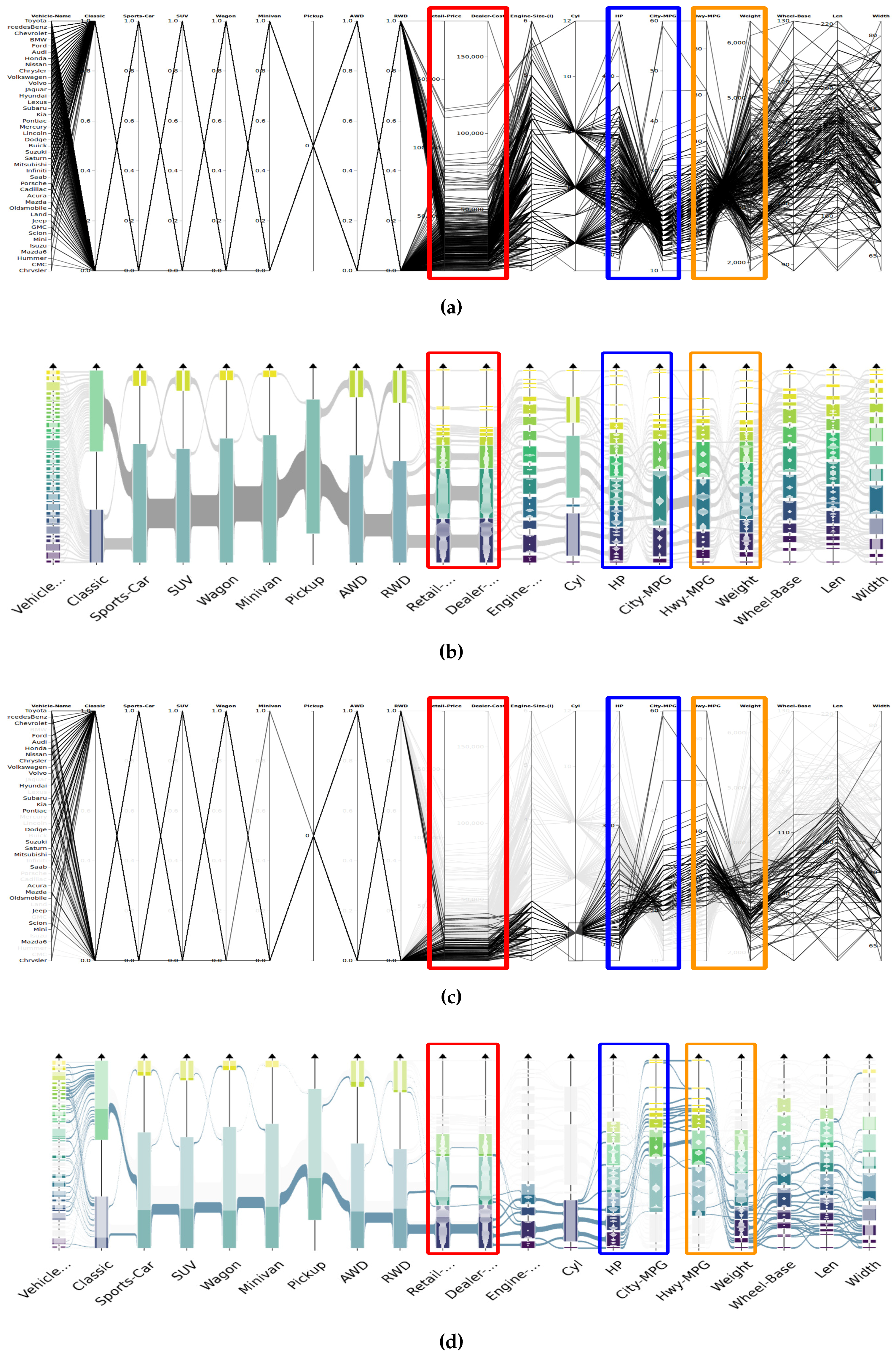
6.1. Comparison to Traditional Parallel Coordinates

The cars dataset represents the characteristics of 400 cars using 20 attributes: the nine first attributes are either categorical (constructor) or boolean value (false is set to 0 and true to 1) while the remaining are integers and reals. The numerical attributes are clustered using a resolution parameter k = 15 while the categorical and boolean attributes are just aggregated by exact match (alphabetical or true/false values).

6.1.1. Gain Overview

At first sight, one can notice on Figure 7 that it is rather easy to figure out the distribution of clusters per attributes with our technique since clusters and meta-links are depicted as thick as the number of elements they represent. Thus, the distribution of elements over clusters for an attribute is one of the first information we obtain when visualizing the clusters. For example if we consider the boolean attributes in Figure 7b (the 8 attributes starting from the second one on the left), elements are clustered in two aggregates (except for the Pickup category), and it is rather straight forward to identify the distribution within each categories. Similarly, it is quite simple to find out the meta-links between one cluster and its neighborhood and in which proportion since meta-link thickness represents the number of elements. It is difficult to obtain the same information on Figure 7a as many lines overlap. This is a well-known limit of classical parallel coordinates and modern state-of-the-art techniques do present solutions to this issue (using density [12], curves[14] for example). If we consider the two attributes of retail price and dealer cost (surrounded in red on Figure 7a,b), we observe with both techniques, line-based and abstracted, that meta-links between the two axes are parallel. This indicates that both attributes of retail price and dealer cost are, to some degree, correlated. On the contrary, the two pairs of axes HorsePower (HP)-City MPG (surrounded in blue) and Hwy MPG-weight (surrounded in yellow) present meta-links that cross in a dense area. That tends to indicate an anti-correlation: high (resp. low) value for one attribute induces low (resp. high) value for the second attribute.

6.1.2. Subset Highlighting

Both techniques make possible to highlight a subset corresponding to continuous values on a dimension and trace the distribution of its elements over all others. While Figure 7c suffers from clutter due to overlaps, our technique makes possible to highlight the selected subset for every attribute and the proportion it represents for each cluster of the plot. For example, selecting cars with less than 4 cylinders (see Figure 7c,d) emphasizes cars with a low retail price, dealer cost, engine size, horsepower, weight, wheel base, length and width. The analysis also indicates that the subset matching the selection also tends to have a lower mileage consumption (city and highway) and matches with city cars which are small and light-weight cars.

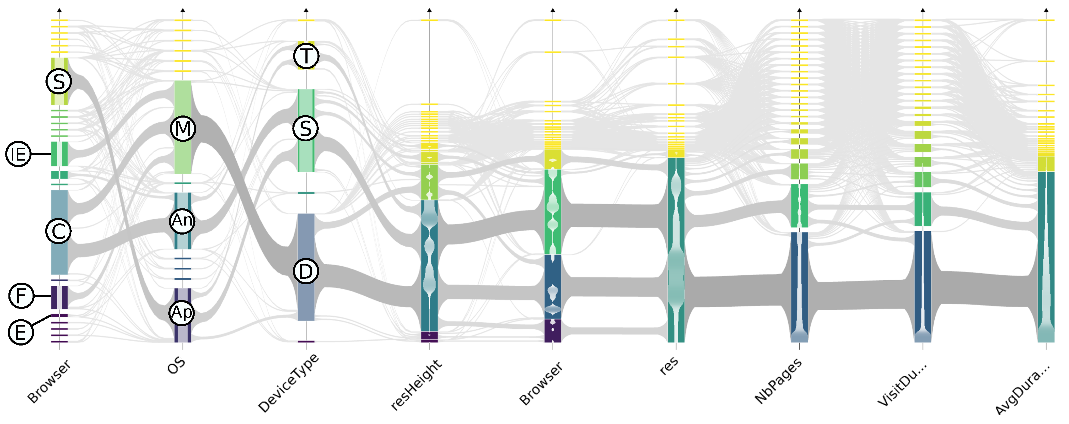
6.2. Large Dataset Visual Analysis

The C2C dataset contains 1.6 billions elements of web traffic data on a C2C (Consumer to Consumer) website (see Figure 8). This dataset contains 9 dimensions where each item is a sequence of pages visited by the same user in a given time. The three first axes represent the user’s browser, OS and device type; the following three are its screen properties (resolution height, width and total resolution). The last ones correspond to the number of visited pages during the session, the session duration and the average time spent per page.
One can easily identify on Figure 9 two major devices corresponding to Desktops and Smartphones and a smaller one, the Tablets (respectively labeled D, S and T). We can notice that users can be distinguished in two equal size categories according to the device they use: either a mobile device (Smartphones or tablets) or desktop device. If we consider the Desktop devices (see Figure 10a), they relate to various resolution sizes and are mainly used with a Microsoft Operating System (labeled M). We can also identify the four major browsers, in growing order of size Chrome, Safari, Firefox and Internet Explorer (respectively labeled C, S , F and IE). If we consider the Smartphones (see Figure 10b), the resolutions are smaller and two main OS are highlighted, the one with the smaller gauge relates to Apple operating systems (labeled Ap) while the bigger one is Android (labeled An). The used browser is largely Safari (labeled S) for Apple and Chrome for Android.
If we analyze this information, we can draw a few conclusions. First, it seems that Microsoft operating systems are mostly used on desktops while their browsers (Internet Explorer and Edge) are not in the mostly used. Second, Apple’s products are mainly used with mobile devices (smart-phones and tablets) and almost solely with the dedicated browser (as highlighted on Figure 9a). Third, Chrome Browser is as much used with desktops than with smart-phones and mainly with Microsoft and Android operating system as emphasized on Figure 9b.
We can also identify a low correlation between resolution width, height and total. The low strength of this correlation is understandable as only higher (resp. lower) total resolution result from high (resp. low) width and height. Medium total resolution can result from high width and low height (or the opposite) which decreases the correlation strength.
These two case studies demonstrate that analyses usually done with traditional parallel coordinates plot can also be performed using our novel abstract-parallel-coordinates technique. While analyses with classical parallel coordinates are element-oriented, using abstracted parallel coordinates, they are aggregate-oriented. This makes sense as abstracted parallel coordinates are dedicated to big data analysis and rather focus on major trends rather than single element analysis. As for any abstract method, the aggregation used, in our case the clustering algorithm and resolution parameters chosen, strongly affect the representation and thus, the possible analyses. Pre-computing the same dataset at various resolution parameter or/and using various algorithms makes possible to refine the analysis but at the expense of storage. Furthermore, using a higher resolution parameter has direct impact on the data transfer size and thus, can affect responsiveness negatively.

7. System Scalability

In our solution, two types of computation occur: pre-computing and on-demand query computation. Pre-computing and on-demand computation are what makes the system interactive, therefore we evaluated response time for pre-computed queries as well as on-demand queries. We also examined the scalability of the pre-processing step and on-demand queries execution times relative to the allocated resources.
Our benchmarks were made using a self-hosted platform composed of 16 computing units, each having 64 GB RAM and 2 × 6 hyper-threaded cores (2.1 GHz). Network capacity within the platform is 1 Gbit/s. Data are transferred on a local network between the server and the platform, as well as between the client and the server. Consequently, all response times were measured from the client perspective, i.e., they include the local network transfer cost from the platform to the server and from the server to the client.

7.1. Implementation Details

On the client side we use WebGL, a web variation of OpenGL, to perform GPU-based computation (using GLSL vertex and fragment shaders) and render visualizations in browsers. More precisely, the client is compiled from C++ to Javascript using emscripten which also binds OpenGL calls to WebGL instructions.
We implemented our back-end system in an Hadoop environment, a data-intensive infrastructure providing distributed storage (HDFS), computing (Spark-MapReduce) and database system (HBase) with horizontal scalability. For on-demand computing, we use Elasticsearch [46], a search system which runs along with the Hadoop components (see Figure 2).
Pre-computation operations (abstraction and prepared selections) are implemented with Spark. The basic of the method is to produce RDDs (for Resilient Distributed Dataset, the main data structure in Spark), where rows represent records with appropriate (key, values) and to retrieve the desired metrics (minimum, count, etc) by reducing values by keys.
In the following, d designates the number of dimensions and n the number of records. Computing the abstraction consists in computing the clusters and meta-links properties from the per-dimension aggregations. These aggregations provide, for each individual record an associated cluster identifier. From there, cluster extrema are obtained by reducing the n · d raw values indexed by a pair ( d i m e n s i o n , c l u s t e r ) .
Using these extrema, we built an RDD (called clusterRDD) by mapping each of the n rows of raw values to a d-tuple of ( c l u s t e r , b i n ) , where the tuple order indicates the dimension. We then transform each row of the clusterRDD into d rows with key ( d i m e n s i o n , c l u s t e r , b i n ) . The distribution and weight of each cluster are then computed by reducing the n · d rows by key. The number of values to process is therefore O ( n · d ) . To count meta-link weights, we map each clusterRDD row to d · ( d 1 ) 2 rows, one for each unique pair of dimensions ( i , j ) . These rows have keys ( i , j , c i , c j ) , where c i and c j are cluster identifiers of dimensions i and j, and with value 1. Reducing by key the resulting RDD gives us the weights of all meta-links. The number of values to process is therefore O ( n · d 2 ) .
Clusters properties and meta-link weights for all the cluster selections are obtained with the same principle as for the abstraction. Since each record contributes to d different cluster selections, each clusterRDD will be transformed into d times more rows than for the abstraction computation. Therefore, cluster properties and meta-link weights computation processes O ( n · d 2 ) and O ( n · d 3 ) values respectively. Similarly, one record will contribute to d · ( d 1 ) 2 meta-links selections. Therefore, the cost to compute cluster properties and meta-link weights for those selections is O ( d 2 ) times larger, i.e., respectively O ( n · d 3 ) and O ( n · d 4 ) .
These different steps use the reduceByKey Spark operation which consists in applying a reducing function onto values grouped by keys. This operation requires a shuffle step to redistribute values based on their keys between partitions before applying the reduce function. This step being memory-consuming, we segmented the cluster and meta-link selections computation in sequential steps so that each step has a computational cost comparable to the abstraction computation one.

7.2. Performance Evaluation Scope

First, we measured pre-computing time which include the clustering, the initial view computation with the preparation of axis rearrangements and single-aggregate selections. Second, we measured the performance of single and compound selection queries (respectively corresponding to prepared queries and on-demand queries). We also examined the scalability of the system by measuring the speedup obtained by allocating more resources for two operations: pre-computing step and on-demand brushing queries. The speedup for p corresponds to the ratio of the execution time using a reference number of computing units (usually one) over those using p computing units. Axis reordering queries were not evaluated as they work similarly to single-aggregate selection queries and have equivalent or better performance.
The outcomes of these experiments depend on different factors. In addition to the number of computing units and the communication overheads, they depend on the chosen dataset and abstraction properties (itself dependent on the clustering and the resolution parameter k).
We considered three types of generated datasets presenting different inter-dimension correlation factors [47], and with size ranging from 10 6 to 10 9 records for 15 dimensions and 15 clusters per dimension. The first type is independent: every pair of dimensions has a close to null correlation factor and close to the maximum number of meta-links between each couple of dimensions (about k 2 ). This type represents the worst case for our system. The second type is correlated, generated to obtain a correlation factor of at least 0.6 between each pair of dimensions. This dataset aims at mimicking the correlation that may be observed in real datasets. The last type has the minimum number of meta-links: k per couple of dimensions, and as such, is the best case. For each test, we average the measured time over three runs.

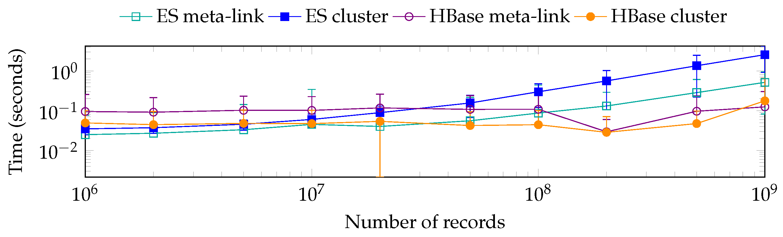
7.3. Pre-Computing Performance

Preparing a dataset consists of computing an abstraction and all single-aggregate (clusters and meta-links) selections. The result of this one-time operation populates HBase with abstract data and prepared queries. When using on-demand computation, an Elasticsearch index is also populated with cluster identifiers for each dimensional components of each record. Pre-computing time measurements (excluding Elasticsearch indexing) are shown in Figure 11a for different data sizes (in number of records) of the three types of dataset. The pre-computation processing is dominated by the computation of all single-aggregate selections. Although we consider the clustering method as parameter that should be chosen in regard of the studied data, we included this step in the measurement. However, it only accounts for about 0.10 % of the total processing time on average.
This processing effectively occurs over pre-aggregated data composed of identical records which are records falling into the exact same cluster for each dimensions (as well as the same cluster histogram bin). These records are considered identical because they are not distinguishable given the interaction tools provided by our system. Due to its properties, the best case dataset is reduced to about 10 · k such identical records (where 10 is the number of inner-cluster histogram bins). Additionally, the best case dataset presents only about k meta-links between each dimensions while correlated and independent have about k 2 , that is k times more. Therefore, about k times more single-aggregate selections are pre-computed for those two later datasets. The difference in number of pre-computation and the size of their input data explains the diverging trend observed on Figure 11a between, on the one side the correlated and independent datasets and on the other side the best case dataset. Indeed, this optimization is not efficient for the correlated and independent datasets (almost no records are identical). On our platform, the pre-computation step takes up to 32 h for datasets of a billion of records. For the largest independent and correlated datasets, the execution time raises up to 24 h.
This computation step runs distributively, hence can be accelerated by increasing the number of computing units participating the task. Figure 11b presents the mean execution time and the corresponding speedup of this step run on the correlated dataset with 10 7 records. The speedup here measures the gain of allocating more executors relative to using a single one. At worst, it appears to be just over 60 % of the optimum, which indicates that the communication overhead is reasonable and that the computation demonstrates good scalability. Thus, while the pre-computation appears to be costly, it is possible to allocate more resources to the platform to efficiently accelerate the processing time.

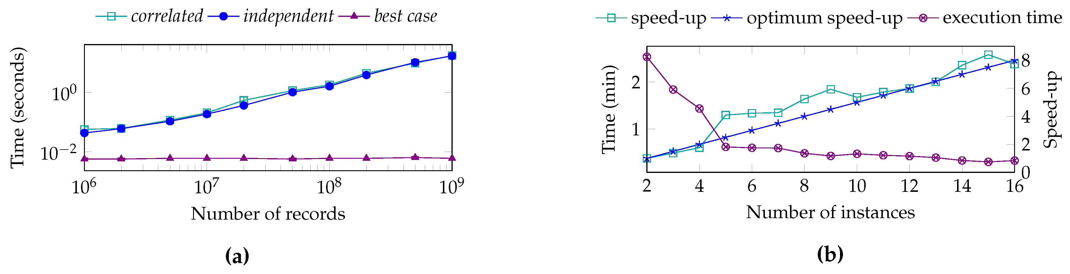
7.4. Prepared Selections Query Performance

To evaluate the performance of single-aggregate selection retrieval, we perform a comparative benchmark between fetching prepared results from HBase and on-demand computation with Elasticsearch (both using 16 computing units). For different dataset types and sizes, we measure response time for selection queries corresponding to each visible elements on an initial display, that is each of its clusters and meta-links. We average the results of the meta-links and clusters independently and examine results for the same operations using Elasticsearch. This way, we can characterize the gain of pre-computing compared to (distributed) on-demand computation. Figure 12 compiles these results for correlated datasets (independent datasets shows similar results). Overall, prepared queries can be retrieved in less than 0.1 s from HBase and the response time does not seem to increase with the dataset size while for Elasticsearch, the response time increases until exceeding the second for the largest datasets. This shows that past a certain size of dataset, there is a significant gain in using pre-computation.

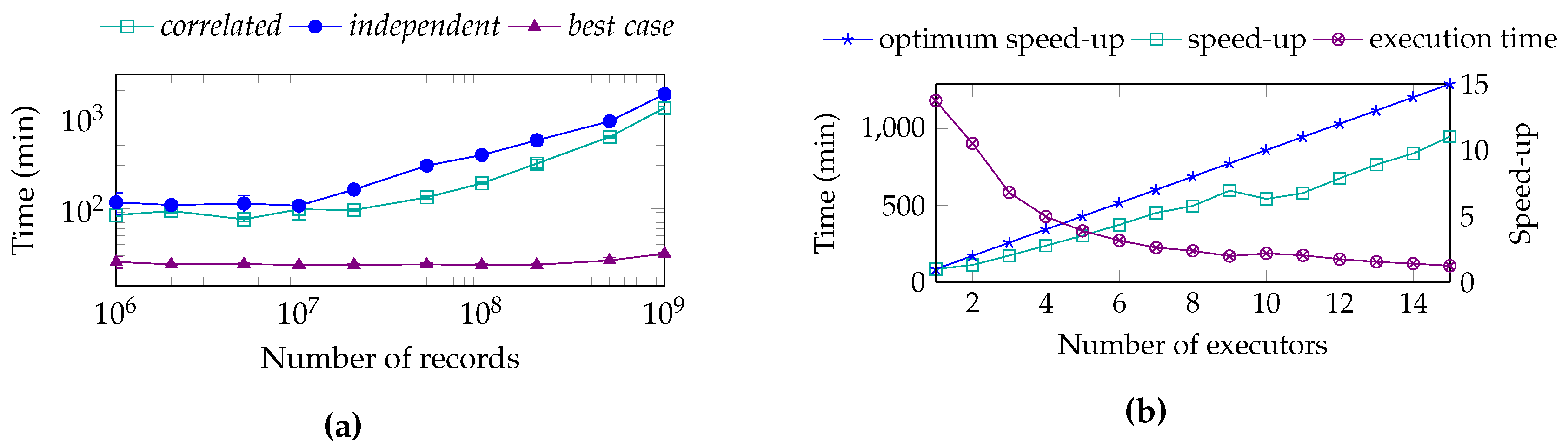
7.5. On-Demand Query Performance

Compound selection queries rely on on-demand processing and operate as a conditional filter followed by an aggregation. As such, they are dependent on the size of the targeted subset of records. Therefore, we are particularly interested in evaluating a cost bound for this operation to ensure good performance. To limit the cost of the aggregation, we query Elasticsearch for at most a subset of half the size of all the dataset by choosing to filter the dataset complement of the original query when it is preferable. In these cases, the server uses the pre-computed full abstraction to compose the original query’s result. We choose to evaluate a higher upper bound for this type of query: the selection of all aggregates at once which means aggregating all clusters and meta-links. This case is presented on Figure 13a. The response times increase with the dataset size, which is expected. For datasets of up to 10 8 items, the response time is lower than one second, however, for upper sizes, the responses times are getting very important. It indicates that the number of computing units is not sufficient to keep up with the aggregating costs for correlated and independent datasets. To ensure sub-second compound selections for this type of datasets and configuration, more resources have to be allocated. The surprisingly low latencies observed for the best case dataset result from the same pre-aggregation treatment of identical records mention above: when populating Elasticsearch indices, only distinct records are inserted. Consequently, all aggregation are applied on smaller data.
As shown, the testing platform shows its limits for the largest datasets used. We measure the speedup gained by using different number of instances in Elasticsearch cluster relative to using only two. Figure 13b, presents the result of the execution time of all possible cluster selection queries on the 2 × 10 8 version of the independent dataset. Here, the speedup appears better than the optimum as it is relative to non-sequential execution. The results indicates that the computing capabilities of the platform are linked to the number of executor with no major loss of performances.

7.6. Discussion

For these experiments, all components (client, platform and server) use local area networks and thus the system is not subjected to world network contingency that could add rather high latencies to transfers. While it is reasonable to consider the server-to-platform connection to be of controlled quality, the main limitation of our experiments is that we cannot not realistically assume a similar connection quality between clients and the server. Nevertheless, bounding data transfer addresses, at least partially, this concern.
However, the results obtained provide some good hints about the capabilities of the system and the pros and cons of beforehand and on-demand computing. Indeed, there is a trade-off between the time consumed by pre-computation and the gain in execution time of using prepared or partially prepared results. In our case, as the data abstraction requires pre-processing, we leveraged that first necessary step by also preparing query results for several interactions. As demonstrated, using pre-processing, we ensure lower response time compared to on-demand computation for single-aggregate selection queries on the largest datasets of our experimentation set. Choosing one strategy or the other for a given query type generally depends on three factors: the available storage, the time allowed for pre-processing and the needs of interactivity i.e., how fast the response-time should be. For the particular case of compound aggregate selections, there is a combinatorial explosion in the number of possible queries which motivates the choice of on-demand computation.
Overall, the experiments shows that on our testing platform, we achieve the targeted sub-second performance for all pre-computed queries: single-aggregate selections and axis reordering queries. Despite pre-computation taking up to 32 h for the largest dataset, the performances depends on several factors: they are closely related to the platform resources, the properties and number of dimensions of the tested data, and the resolution parameter. Since our experimentation demonstrated the horizontal scalability of the system, providing more resources would induce better performances seamlessly.

8. Conclusions & Future Work

In this paper, we present a system for interactive visual exploration of multidimensional data with a parallel coordinates representation. In order to support the visual exploration of large data sets, our system addresses three aspects of scalable visualization systems: perceptual scalability, interactive scalability and remoteness. We employ pre-processing and on-demand computation to bring interactivity to an abstract parallel coordinates representation, integrated in a client-server visualization system. A distant infrastructure handle distributed computing and data pre-aggregation and on-demand aggregation while a web-based remote visualization client for parallel rendering provides an interactive visualization that respect the perceptual scalability. The client is provided with various interaction tools to handle equivalent data exploration and data analyzes capabilities as state-of-the-art techniques. Among theses interactions, two of them (axis reordering and subset highlighting) imply data transfers between the infrastructure and the rendering client. Our system guarantees upper bounds for these transfers, ensuring interactivity and responsiveness of the rendering client. We present and evaluate an implementation of the back-end using using the Hadoop ecosystem (HDFS and HBase), Spark and Elasticsearch. The results indicate a good scalability and reasonable responsiveness of our system on up to a billion of items.
A first interesting work to pursue is thoroughly studying real-time distributed computing scalability of different technologies to ameliorate the pre-computing step in our solution. Lower preparation times would let users change dataset and tune clustering parameters in a more responsive way. Secondly, to bypass interaction latencies, prediction and pre-fetching [48] could be investigated. Other selection interactions could be implemented to further refine the highlighted subset: for instance selecting multiple ranges along one dimension or make logic operations between those selections. We also intend to examine how abstract parallel coordinates could be extended to a multi-scale visualization. Namely, how to create different levels of details and enable their exploration while guaranteeing a bounded number of displayed and transferred items.

Acknowledgments

This work has been carried out as part of SpeedData project supported by the French Investissement d’Avenir Program (Big Data—Cloud Computing topic) managed by Direction Générale des Entreprises (DGE) and BPIFrance.

Author Contributions

G.R., T.J., J.S. and R.B. performed the pipeline design, implementation and client-side data processing. F.L. performed the server-side data processing, system interface and management, and benchmark experiments. The overall work have been done under the supervision of R.B.. G.R. and J.S. wrote the paper and R.B. and D.A. performed the internal reviewing process.

Conflicts of Interest

The authors declare no conflict of interest.

References and Note

  1. Elmqvist, N.; Dragicevic, P.; Fekete, J. Rolling the Dice: Multidimensional Visual Exploration using Scatterplot Matrix Navigation. IEEE Trans. Vis. Comput. Gr. 2008, 14, 1148–1539. [Google Scholar] [CrossRef] [PubMed]
  2. Alpern, B.; Carter, L. The Hyperbox. In Proceedings of the 2nd IEEE Computer Society Press: Los Alamitos Conference on Visualization ’91, San Diego, CA, USA, 22–25 October 1991; pp. 133–139. [Google Scholar]
  3. Kandogan, E. Star coordinates: A multi-dimensional visualization technique with uniform treatment of dimensions. In Proceedings of the IEEE Information Visualization Symposium, Salt Lake City, UT, USA, 8–13 October 2000; Volume 650, p. 22. [Google Scholar]
  4. Andrews, D.F. Plots of high-dimensional data. Biometrics 1972, 28, 125–136. [Google Scholar] [CrossRef]
  5. Inselberg, A. The plane with parallel coordinates. Vis. Comput. 1985, 1, 69–91. [Google Scholar] [CrossRef]
  6. Wegman, E.J. Hyperdimensional Data Analysis Using Parallel Coordinates. J. Am. Stat. Assoc. 1990, 85, 664–675. [Google Scholar] [CrossRef]
  7. Heinrich, J.; Weiskopf, D. State of the art of parallel coordinates. STAR Proc. Eurogrph. 2013, 2013, 95–116. [Google Scholar]
  8. Raidou, R.G.; Eisemann, M.; Breeuwer, M.; Eisemann, E.; Vilanova, A. Orientation-Enhanced Parallel Coordinate Plots. IEEE Trans. Vis. Comput. Graph. 2016, 22, 589–598. [Google Scholar] [CrossRef] [PubMed]
  9. Ellis, G.; Dix, A. Enabling Automatic Clutter Reduction in Parallel Coordinate Plots. IEEE Trans. Vis. Comput. Graph. 2006, 12, 717–724. [Google Scholar] [CrossRef] [PubMed]
  10. McDonnell, K.T.; Mueller, K. Illustrative Parallel Coordinates. Comput. Graph. Forum 2008, 27, 1031–1038. [Google Scholar] [CrossRef]
  11. Baldi, P.; Sadowski, P.; Whiteson, D. Searching for exotic particles in high-energy physics with deep learning. Nat. Commun. 2014, 5, 4308. [Google Scholar] [CrossRef] [PubMed]
  12. Zhou, H.; Cui, W.; Qu, H.; Wu, Y.; Yuan, X.; Zhuo, W. Splatting the Lines in Parallel Coordinates; Blackwell Publishing Ltd.: Oxford, UK, 2009; Volume 28, pp. 759–766. [Google Scholar]
  13. Nhon, D.T.; Wilkinson, L.; Anand, A. Stacking Graphic Elements to Avoid Over-Plotting. IEEE Trans. Vis. Comput. Graph. 2010, 16, 1044–1052. [Google Scholar]
  14. Zhou, H.; Yuan, X.; Qu, H.; Cui, W.; Chen, B. Visual Clustering in Parallel Coordinates; Blackwell Publishing Ltd.: Oxford, UK, 2008; Volume 27, pp. 1047–1054. [Google Scholar]
  15. Theisel, H. Higher Order Parallel Coordinates. In Proceedings of the 5th International Fall Workshop Vision, Modeling and Visualization, Saarbrücken, Germany, 22–24 November 2000; pp. 415–420. [Google Scholar]
  16. Graham, M.; Kennedy, J. Using curves to enhance parallel coordinate visualisations. In Proceedings of the 7th International Conference on Information Visualization, London, UK, 18 July 2003; pp. 10–16. [Google Scholar]
  17. Ellis, G.P.; Dix, A.J. A Taxonomy of Clutter Reduction for Information Visualisation. IEEE Trans. Vis. Comput. Graph. 2007, 13, 1216–1223. [Google Scholar] [CrossRef] [PubMed]
  18. Fua, Y.; Ward, M.O.; Rundensteiner, E.A. Hierarchical Parallel Coordinates for Exploration of Large Datasets. In Proceedings of the IEEE Visualization ’99, San Francisco, CA, USA, 24–29 October 1999; pp. 43–50. [Google Scholar]
  19. Andrienko, G.; Andrienko, N. Parallel Coordinates for Exploring Properties of Subsets. In Proceedings of the Second IEEE Computer Society International Conference on Coordinated & Multiple Views in Exploratory Visualization, Washington, DC, USA, 13 July 2004; pp. 93–104. [Google Scholar]
  20. Artero, A.O.; de Oliveira, M.C.F.; Levkowitz, H. Uncovering Clusters in Crowded Parallel Coordinates Visualizations. In Proceedings of the 10th IEEE Symposium on Information Visualization (InfoVis 2004), Austin, TX, USA, 10–12 October 2004; pp. 81–88. [Google Scholar]
  21. Johansson, J.; Cooper, M.D. A Screen Space Quality Method for Data Abstraction. Comput. Graph. Forum 2008, 27, 1039–1046. [Google Scholar] [CrossRef]
  22. Johansson, J.; Ljung, P.; Jern, M.; Cooper, M.D. Revealing Structure within Clustered Parallel Coordinates Displays. In Proceedings of the IEEE Symposium on Information Visualization (InfoVis 2005), Minneapolis, MN, USA, 23–25 October 2005; Stasko, J.T., Ward, M.O., Eds.; IEEE Computer Society: Washington, DC, USA, 2005; p. 17. [Google Scholar]
  23. Luo, Y.; Weiskopf, D.; Zhang, H.; Kirkpatrick, A.E. Cluster Visualization in Parallel Coordinates Using Curve Bundles. IEEE Trans. Vis. Comput. Graph. 2008, 18, 1–12. [Google Scholar]
  24. Siirtola, H. Direct manipulation of parallel coordinates. In Proceedings of the IEEE International Conference on Visualization, London, UK, 19–21 July 2000; pp. 373–378. [Google Scholar]
  25. Beham, M.; Herzner, W.; Gröller, M.E.; Kehrer, J. Cupid: Cluster-Based Exploration of Geometry Generators with Parallel Coordinates and Radial Trees. IEEE Trans. Vis. Comput. Graph. 2014, 20, 1693–1702. [Google Scholar] [CrossRef] [PubMed]
  26. Van Long, T.; Linsen, L. MultiClusterTree: Interactive Visual Exploration of Hierarchical Clusters in Multidimensional Multivariate Data; Blackwell Publishing Ltd.: Oxford, UK, 2009; Volume 28, pp. 823–830. [Google Scholar]
  27. Palmas, G.; Bachynskyi, M.; Oulasvirta, A.; Seidel, H.P.; Weinkauf, T. An edge-bundling layout for interactive parallel coordinates. In Proceedings of the IEEE Pacific Visualization Symposium, Yokohama, Japan, 4–7 March 2014; pp. 57–64. [Google Scholar]
  28. Novotny, M.; Hauser, H. Outlier-Preserving Focus + Context Visualization in Parallel Coordinates. IEEE Trans. Vis. Comput. Graph. 2006, 12, 893–900. [Google Scholar] [CrossRef] [PubMed]
  29. Kosara, R.; Bendix, F.; Hauser, H. Parallel sets: Interactive exploration and visual analysis of categorical data. IEEE Trans. Vis. Comput. Graph. 2006, 12, 558–568. [Google Scholar] [CrossRef] [PubMed]
  30. Lex, A.; Streit, M.; Partl, C.; Kashofer, K.; Schmalstieg, D. Comparative analysis of multidimensional, quantitative data. IEEE Trans. Vis. Comput. Graph. 2010, 16, 1027–1035. [Google Scholar] [CrossRef] [PubMed]
  31. Liu, Z.; Jiang, B.; Heer, J. imMens: Real-time Visual Querying of Big Data. Comput. Graph. Forum 2013, 32, 421–430. [Google Scholar] [CrossRef]
  32. Rübel, O.; Prabhat; Wu, K.; Childs, H.; Meredith, J.S.; Geddes, C.G.R.; Cormier-Michel, E.; Ahern, S.; Weber, G.H.; Messmer, P.; et al. High performance multivariate visual data exploration for extremely large data. In Proceedings of the ACM/IEEE Conference on High Performance Computing, Austin, TX, USA, 15–21 November 2008; p. 51. [Google Scholar]
  33. Perrot, A.; Bourqui, R.; Hanusse, N.; Lalanne, F.; Auber, D. Large interactive visualization of density functions on big data infrastructure. In Proceedings of the 5th IEEE Symposium on Large Data Analysis and Visualization (LDAV), Chicago, IL, USA, 25–26 October 2015; pp. 99–106. [Google Scholar]
  34. Chan, S.M.; Xiao, L.; Gerth, J.; Hanrahan, P. Maintaining interactivity while exploring massive time series. In Proceedings of the IEEE Symposium on Visual Analytics Science and Technology, Columbus, OH, USA, 19–24 October 2008; pp. 59–66. [Google Scholar]
  35. Piringer, H.; Tominski, C.; Muigg, P.; Berger, W. A Multi-Threading Architecture to Support Interactive Visual Exploration. IEEE Trans. Vis. Comput. Graph. 2009, 15, 1113–1120. [Google Scholar] [CrossRef] [PubMed]
  36. Elmqvist, N.; Fekete, J.D. Hierarchical Aggregation for Information Visualization: Overview, Techniques, and Design Guidelines. IEEE Trans. Vis. Comput. Graph. 2010, 16, 439–454. [Google Scholar] [CrossRef] [PubMed]
  37. Wu, K.; Ahern, S.; Bethel, E.W.; Chen, J.; Childs, H.; Cormier-Michel, E.; Geddes, C.; Gu, J.; Hagen, H.; Hamann, B.; et al. FastBit: Interactively searching massive data. J. Phys. 2009, 180, 012053. [Google Scholar] [CrossRef]
  38. Card, S.K.; Robertson, G.G.; Mackinlay, J.D. The information visualizer, an information workspace. Proceeding of the CHI Conference on Human Factors in Computing Systems, New Orleans, LA, USA, 27 April–2 May 1991; Robertson, S.P., Olson, G.M., Olson, J.S., Eds.; ACM: New York, NY, USA, 1991; pp. 181–186. [Google Scholar]
  39. Godfrey, P.; Gryz, J.; Lasek, P. Interactive Visualization of Large Data Sets. IEEE Trans. Knowl. Data Eng. 2016, 28, 2142–2157. [Google Scholar] [CrossRef]
  40. Steinley, D. K-means clustering: A half-century synthesis. Br. J. Math. Stat. Psychol. 2006, 59, 1–34. [Google Scholar] [CrossRef] [PubMed]
  41. Ester, M.; Kriegel, H.; Sander, J.; Xu, X. A Density-Based Algorithm for Discovering Clusters in Large Spatial Databases with Noise. In Proceedings of the Second International Conference on Knowledge Discovery and Data Mining (KDD-96), Portland, OR, USA, 1996; pp. 226–231. [Google Scholar]
  42. Riehmann, P.; Hanfler, M.; Froehlich, B. Interactive Sankey Diagrams. In Proceedings of the IEEE Symposium on Information Visualization (InfoVis 2005), Minneapolis, MN, USA, 23–25 October 2005; Stasko, J.T., Ward, M.O., Eds.; IEEE Computer Society: Washington, DC, USA, 2005; p. 31. [Google Scholar]
  43. Wegman, E.J.; Luo, Q. High Dimensional Clustering Using Parallel Coordinates and the Grand Tour. In Classification and Knowledge Organization: Proceedings of the 20th Annual Conference of the Gesellschaft für Klassifikation e.V., University of Freiburg, Baden-Württemberg, Germany, 6–8 March 1996; Klar, R., Opitz, O., Eds.; Springer: Berlin/Heidelberg, Germany, 1997; pp. 93–101. [Google Scholar]
  44. Ward, M.O.; Grinstein, G.G.; Keim, D.A. Interactive Data Visualization—Foundations, Techniques, and Applications; A K Peters: Natick, MA, USA, 2010. [Google Scholar]
  45. Auber, D.; Chiricota, Y.; Delest, M.; Domenger, J.; Mary, P.; Melançon, G. Visualisation de graphes avec Tulip: Exploration interactive de grandes masses de données en appui à la fouille de données et à l’extraction de connaissances. In Proceedings of the Extraction et Gestion des Connaissances (EGC’2007), Actes des Cinquièmes Journées Extraction et Gestion des Connaissances, Namur, Belgique, 23–26 January 2007; pp. 147–156. [Google Scholar]
  46. Elasticsearch, 1999.
  47. Börzsönyi, S.; Kossmann, D.; Stocker, K. The Skyline Operator. In Proceedings of the 17th International Conference on Data Engineering; IEEE Computer Society: Washington, DC, USA, 2001; pp. 421–430. [Google Scholar]
  48. Doshi, P.R.; Rundensteiner, E.A.; Ward, M.O. Prefetching for Visual Data Exploratio. In Proceedings of the Eighth International Conference on Database Systems for Advanced Applications (DASFAA ’03), Kyoto, Japan, 26–28 March 2003; pp. 195–202. [Google Scholar]
Figure 1. Traditional parallel coordinates. (a) Representation of a four-dimensional record X with a polyline (b) Example of clutter produced by the crossing and overlapping of many lines.
Informatics 04 00021 g001
Figure 2. System components. Data processing steps using Spark occur once and consist in the clustering of dimension values, forming the abstraction (clusters and meta-links) for the initial view and all axis ordering, as well as preparing all single-aggregate selections. The server interface communicates with two types of storage system to answer queries received from the rendering client, one holding prepared data, the other processing aggregation on-demand.
Informatics 04 00021 g002
Figure 3. Both implemented visual encodings for the same abstraction ( k = 30 ). On top, the distribution encoding; on the bottom, the interval encoding. Surrounded in red: the inner-cluster smoothed histogram view.
Informatics 04 00021 g003
Figure 4. Comparison of the two visual encodings proposed for abstract parallel coordinates compared to the line-based version displayed on (a). On (a), ① four elements forming the example cluster and ② two sets of connections forming two example meta-links. On (b), cluster and meta-links size encodes their weight. Meta-links anchor points on clusters are sorted relative to their destination to limit crossings as shown on ③. On (c), cluster sizes correspond to their interval size. Meta-link colors and size respectively depends on their weight and ends. They are depth sorted by weight and attached on each cluster ends to the highest density point as represented on ③. On both (b) and (c), the inner-cluster smoothed histogram is represented on ③. Finally, ④ shows that inter-cluster intervals can be compared, per-axis, on both encodings.
Informatics 04 00021 g004
Figure 5. Two selection views on a C2C dataset described in the next section. Here, items are visiting session on a website. Selecting an aggregate (cluster or meta-link) triggers the highlight of the selected subset through all the displayed axes. The inner-cluster histograms are also updated according to the selection. (a) Selection of the smartphone category (on DeviceType); (b) Selection of the higher range of values (between 37 and 300) on the NbPages axis which relates to the number of visited pages.
Informatics 04 00021 g005
Figure 6. The modification of the two spacings, inter- and intra-axis, allows to tune the representation to get the best ratio depending on the user interest. Thus, we can go from no spaces at all, providing a stacked-histogram (bottom left), to a representation that rather focuses on relative distance between clusters and elements distribution between axes (top right).
Informatics 04 00021 g006
Figure 7. Cars dataset: (a,b) show an overview of the dataset; (c,d) are selections of the cars with less than 4 cylinders; (ac) use the traditional parallel coordinates implementation of the Tulip software [45] and (bd) use our technique.
Informatics 04 00021 g007
Figure 8. C2C website dataset overview with k = 30 (max. number of clusters per attributes). For this dataset, each item is a sequence of pages visited by the same user in a given time. The dataset represents various information collected during visitors navigation : system and device information (OS, browser, device, screen resolution) and navigation information (number of page visited, visit duration and average time spend per pages). The labeled clusters correspond to clusters described in the use case for the browser axis (Edge—E, Firefox—F, Chrome—C, Internet Explorer—E and Safari—S), for the OS axis (Apple—Ap, Android—An and Microsoft—M), and for the Device type (Desktop—D, Smartphone—S and Tablet—T).
Informatics 04 00021 g008
Figure 9. Subset highlighting on the C2C website dataset with k = 30 : Selecting an aggregate highlights the subset over all the plot. (a) Selection of Apple Operating System (iOS or macOS) shows that users only use Safari browser (S) and mainly for mobile devices : tablets (T) and smartphones (S); (b) Selection of Chrome browser (C) highlights users using either desktop devices (D) and smartphone devices (S) and using the corresponding operating systems: Microsoft (M) and android (An).
Informatics 04 00021 g009
Figure 10. Subset selection: selecting an aggregate highlights the subset over all the plot. (a) Selection of desktop devices (D) highlights users using mainly Microsoft (M) operating system and Chrome (C), Internet Explorer (IE) and Firefox (F) browsers; (b) Selection of smartphone devices (S) highlights users using almost equally Android and Apple operating systems and the dedicated browsers (resp. Chrome (C) and Safari (S).
Informatics 04 00021 g010
Figure 11. Performance evaluations for the pre-computation step (clustering, clusters and meta-links, single-aggregate selections and insertion into HBase). (a) Execution time for the three datasets and varying number of records; (b) Scalability evaluation for the correlated dataset with 10 7 records. The speedup is relative to a sequential execution.
Informatics 04 00021 g011
Figure 12. Prepared data fetching and on-demand computing execution times for identical queries. Here response time was measured for all possible single-aggregate selection o(clusters and meta-links) on an initial view of correlated datasets with varying number of records.
Informatics 04 00021 g012
Figure 13. Performance evaluations for the on-demand computation model using Elasticsearch. (a) Upper bound for all on-demand queries, corresponding to computing the total initial view for varying dataset types and number of records; (b) Scalability of on-demand queries, tested on cluster-selection queries for an independent dataset with 2 × 10 8 records. The speedup is relative to using two instances.
Informatics 04 00021 g013

