Hybrid Multifractal-Based Machine Learning Framework for Glaucoma Diagnostics from Retinal Images

Abstract

Glaucoma is a leading cause of irreversible vision loss, and its early diagnosis remains critically important yet challenging. Traditional assessment based on the cup-to-disc ratio is often insufficient at early stages, whereas the retinal vascular network can provide additional quantitative biomarkers. This study develops and validates a binary classification method for distinguishing healthy from glaucomatous fundus images by combining deep-learning-based vessel segmentation, fractal and multifractal analysis, and textural features. The public ORIGA dataset is utilized. Images are converted to grayscale using three alternative approaches, followed by Gray-Level Co-occurrence Matrix texture analysis and fractal analysis based on the differential box-counting method. Vessel segmentation is implemented via a U-Net neural network trained on a combination of public datasets, after which multifractal analysis is performed on the resulting binary masks. The extracted features are used to train and compare several machine learning models with hyperparameter optimization. The best-performing model among ONH-based features (Random Forest) achieves 75.00%; however, a logistic regression model using multifractal parameters and CDR reaches 86.17%, substantially outperforming the CDR-only baseline (66.15%). Notably, while classical fractal dimension shows only marginal differences (1–2% relative change) between groups, multifractal parameters reveal distinct changes: the multifractal spectrum width $\Delta \alpha$ increases markedly and the minimum singularity exponent ${\alpha }_{\min }$ decreases in glaucomatous eyes, indicating increased heterogeneity of the vascular network. These findings suggest that multifractal characteristics of the vascular network can serve as reliable and sensitive biomarkers for automated glaucoma screening, offering clear advantages over classical fractal analysis.

1. Introduction

Research on glaucoma has a long tradition in ophthalmology. Currently, one of the common causes of vision loss is the development of glaucoma. The progression of this disease is often asymptomatic, which complicates timely diagnosis. This is the field of study that deals with pathological changes in glaucoma, which include increased intraocular pressure, thinning of the retinal nerve fiber layer, loss of ganglion cells, neuroretinal rim thinning, and degradation of capillary vessels. These structural changes can be visualized on fundus images, making them promising tools for large-scale screening.

Regular glaucoma screening is essential to prevent irreversible vision loss. However, this leads to myriad problems in clinical practice. Existing diagnostic methods based on fundus images either require manual analysis by highly qualified specialists, which can be subjective and labor-intensive, or involve automated approaches that currently lack sufficient accuracy and generalization ability for widespread deployment.

One effective method for diagnosing glaucoma is calculating the cup-to-disc ratio (CDR). However, the main problem is that glaucoma is characterized not only by changes in the optic disc but also by diffuse thinning of the peripapillary retinal nerve fiber layer and degradation of the capillary network. These vascular changes may serve as additional biomarkers for diagnosing pathological alterations, yet they remain understudied.

Traditional diagnosis based on calculating the cup-to-disc ratio is often insufficiently effective in the early stages. A further problem is that automated tools for rapid and objective assessment of the retinal vascular network are sparsely represented in the literature. Most studies focus on analyzing the macular region or the optic disc, while the diagnostic potential of the retinal vasculature in glaucoma remains understudied. This gap motivates the present research.

In [1,2], the authors provided a comprehensive review of deep learning methods for binary classification and segmentation of the optic disc region. They note that despite the widespread use of methods for analyzing disc shape and excavation, the combination of precise vascular segmentation followed by textural analysis is applied infrequently. Many existing works focus on analyzing the geometric parameters of the disc or use end-to-end classification models without extracting interpretable biomarkers. Ref. [3] presented a comprehensive survey of automated detection methods for diabetic retinopathy, highlighting the growing role of texture-based and fractal-based features in retinal image analysis.

The successful application of deep learning methods for glaucoma diagnosis is confirmed by several studies [4,5,6,7,8,9,10,11,12,13,14]. For instance, the authors of [4] demonstrated that an ensemble of neural network models for optic disc segmentation showed significant superiority over traditional approaches. A CAD system for binary classification using a modified pelican optimization-based extreme learning machine has been proposed in [13]. A deep learning algorithm demonstrating effectiveness on ethnically diverse datasets has been reported in [14]. These works confirm the potential of automated methods; however, none of them combine vessel segmentation with multifractal analysis.

In addition, many biomedical researchers apply fractal and multifractal analysis algorithms. This toolkit allows for the quantitative assessment of structural complexity. A foundational review of fractal analysis of the retinal vascular tree has been provided in [15], demonstrating that fractal dimension can serve as a quantitative descriptor of vascular architecture. Our previous work [16] successfully applied fractal analysis combined with neural networks for the classification of lung CT images, demonstrating the translational potential of this methodology across different medical imaging modalities. A key factor influencing quality is pre-processing, which may involve frequency transformation, noise reduction, contrast enhancement, or morphological operations such as binarization.

There is a wide range of methods for estimating fractal and multifractal characteristics. They can be based on counting covering elements (box-counting) at various scales or on analyzing the distribution of pixel brightness [17]. The choice of a specific method also determines pre-processing requirements: classical box-counting applies to binary images, while its differential modifications work with grayscale images. The authors of [18] performed multifractal analysis of human retinal vessels and showed that multifractal parameters provide richer information about vascular morphology than classical fractal dimension alone.

The effectiveness of combining grayscale conversion methods, GLCM texture analysis, and the differential box-counting method has been demonstrated not only in technical applications but also in related biomedical tasks. For example, three methods have been used in [19] for converting images to monochrome format in conjunction with GLCM parameters and the differential box-counting algorithm. The authors of [20] applied a similar approach for quantitative assessment of corrosion damage. The success of these studies justifies the promise of applying such a methodology to retinal image analysis.

Classical fractal analysis has a significant limitation: it characterizes the entire structure with only a single numerical value. In situations where visually different patterns yield the same dimension, this approach loses its discriminative power. One way to overcome this limitation is to employ multifractal analysis, which characterizes structural heterogeneity through a set of generalized Rényi dimensions. A recent meta-analysis has summarized the current evidence on fractal dimension in retinal pathology, motivating further exploration of advanced fractal-based descriptors for glaucoma diagnostics [21].

The application of multifractal analysis in medical imaging demonstrates its high diagnostic potential. In [22], the multifractal spectrum of lung CT images was used to quantitatively track the progression of pneumonia. The authors of [23] applied multifractal analysis to retinal images and, combined with machine learning, achieved high accuracy in classifying pathologies. In [24], researchers demonstrated that combining structural and non-structural features, including texture-based parameters, improves glaucoma detection performance. These studies confirm the feasibility of a multifractal approach for analyzing structural changes in eye diseases.

One of the key challenges identified in contemporary research on AI in ophthalmology is the insufficient transparency of diagnostic decisions. In their systematic review, the authors of [25] emphasized that despite achieving high accuracy (up to 98.3%) and AUC (up to 0.99), deep learning models often operate as “black boxes,” hindering clinicians’ understanding of diagnostic rationale. This creates significant barriers to clinical implementation, where decision justification is critical.

Recent studies have demonstrated the effectiveness of deep convolutional neural networks for ocular disease diagnosis. For instance, Al Jbaar and Dawwd [26] proposed parallel embedded architectures based on VGG16 and custom lightweight networks, achieving accuracy of up to 96% on the ODIR dataset for multi-label ocular disease detection.

In contrast, the authors note that tabular data combined with interpretable machine learning methods (logistic regression, Random Forest, SVM) not only achieves comparable accuracy but also enables identification of the most significant diagnostic factors. Building on this approach, the present study applies fractal and texture analysis to extract quantitative features that, unlike hidden layers of neural networks, are directly interpretable. This allows for tracing the relationship between structural characteristics of ocular tissues and the diagnostic conclusion, providing necessary transparency for clinical application.

The wide range of accuracy values (76–98%) observed in the literature indicates that high accuracy alone does not guarantee clinical value. As Shahriari et al. emphasize, interpretability remains critically important, particularly when employing “black boxes” in the form of deep neural networks.

The methodology of this study represents a multi-stage ensemble approach combining preprocessing, textural, fractal, and multifractal analysis with subsequent machine learning classification. Specifically, we propose an interpretable multifractal–textural ensemble for glaucoma diagnosis.

To our knowledge, no previous research has investigated such an ensemble. The key contribution of this work is the solution it provides. This study is the first to integrate (i) three alternative grayscale conversion strategies for GLCM-based texture analysis, (ii) differential box-counting fractal dimension of the optic nerve head, and (iii) multifractal spectrum parameters of U-Net-segmented vessels within a single interpretable machine learning framework for glaucoma classification.

At the initial stage, the original RGB images are divided into two domains: full retinal images and extracted optic nerve head (ONH) regions. For each domain, conversion to grayscale is performed using three alternative methods to enable comparative analysis of their impact on classification accuracy. The obtained monochrome images are filtered (median and Gaussian) to minimize noise and artifacts.

For all filtered monochrome images, the Gray-Level Co-occurrence Matrix (GLCM) is calculated, from which Haralick textural features are extracted: contrast, correlation, energy, homogeneity, and entropy. These features characterize the microstructure of the retinal tissue and the ONH.

For the optic nerve head crops, the differential box-counting method is applied. The choice of this method is due to its ability to work with grayscale images without prior binarization, preserving information about brightness gradients within the ONH structure. As a result, fractal dimension is computed as a quantitative measure of disc morphological complexity.

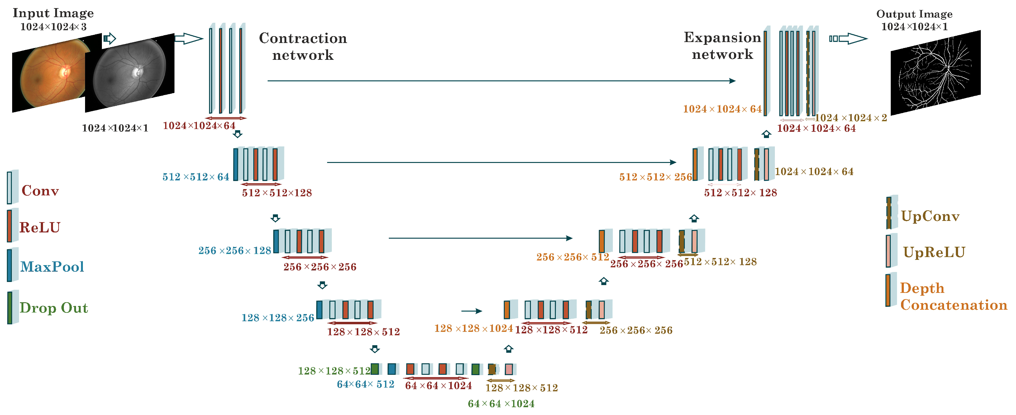
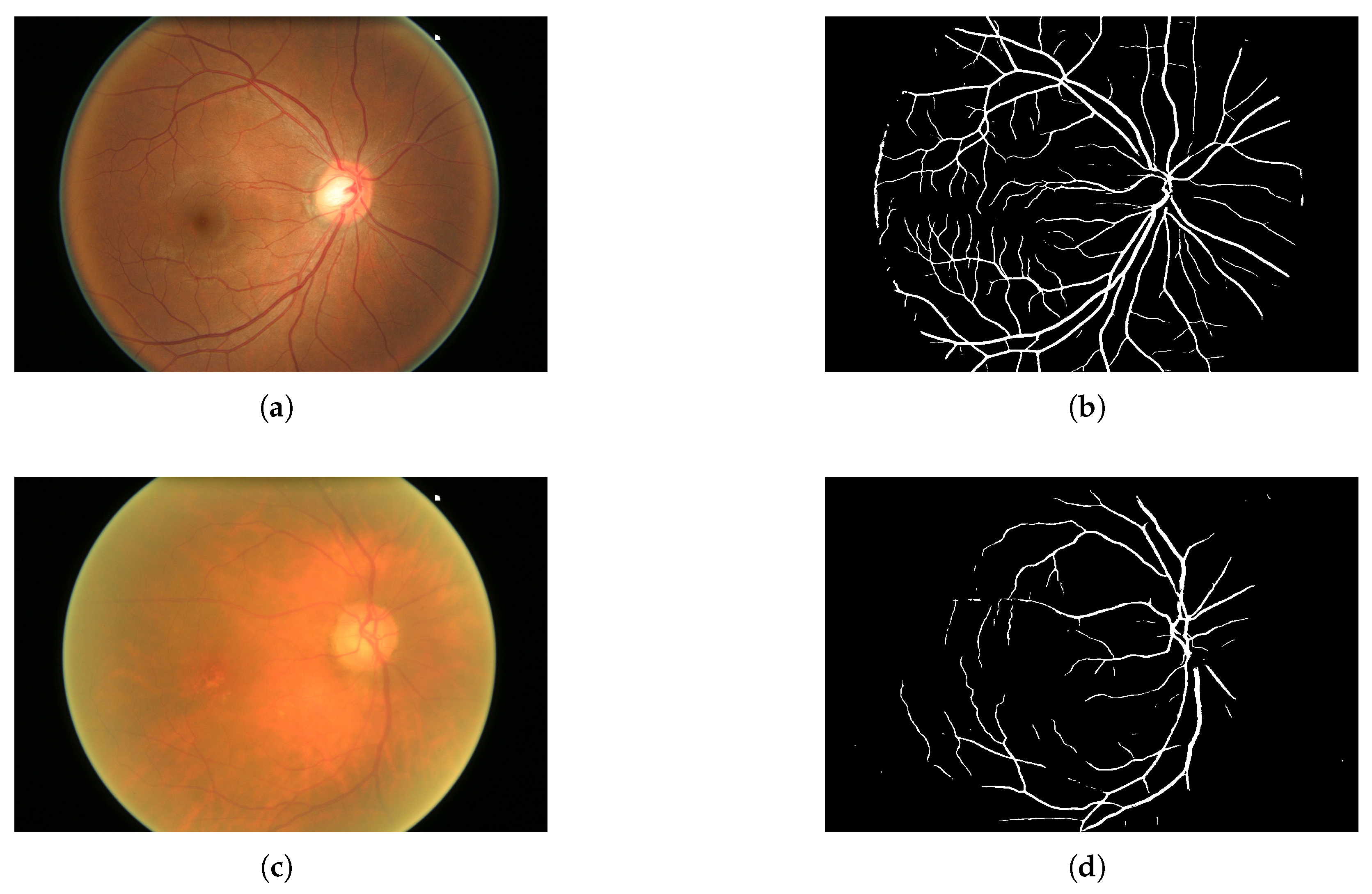
The analysis of full retinal images includes a critical step: segmentation of the vascular bed. Preliminary testing of classical morphological processing methods revealed insufficient effectiveness in segmenting thin capillaries. To overcome this problem, the U-Net neural network architecture [27] was configured and trained on labeled data. The choice of U-Net is justified by its proven effectiveness in biomedical segmentation tasks with limited training data. This approach improved segmentation completeness of peripapillary vessels, which play a key role in glaucoma pathogenesis. Based on the binary masks obtained after segmentation, multifractal analysis is performed, yielding scaling characteristics that capture the heterogeneity and complexity of the vascular architecture.

At the final stage, a combined feature table is formed, including GLCM textures (for all images), DBC fractal dimension (for ONH crops), and multifractal parameters (for vessel masks). The resulting dataset is used for training and comparative analysis of several machine learning models (logistic regression, Support Vector Machine, Random Forest, Gradient Boosting). Model performance is evaluated on a held-out test set using accuracy, precision, recall, and F1-score for the binary classification task (“normal/glaucoma”).

The remainder of this paper is organized as follows: Section 2 describes the dataset, preprocessing steps, U-Net segmentation, fractal and multifractal analysis methods, and the machine learning classification pipeline. Section 3 presents the experimental results and discusses their implications, including segmentation quality, feature extraction outcomes, and classification performance. Section 4 concludes this paper with a summary of the findings and directions for future work.

2. An Ensemble Framework for Retinal Image Feature Extraction and Classification

2.1. Retinal Fundus Datasets

This study utilized several publicly available datasets for analysis, model training, and validation.

For binary classification of healthy and glaucomatous fundus images, the ORIGA dataset [28] was employed. Obtained from the Kaggle repository under an open license, this dataset comprises 650 RGB fundus images with a resolution of $3072\times 2048$ pixels. The class distribution includes 482 normal and 168 glaucomatous images (normal–glaucoma ≈ 2.87:1). The dataset was randomly split into training (60%), validation (20%), and test (20%) sets using stratified sampling to preserve the class distribution. In addition to the images, the dataset provides cup-to-disc ratio values and pre-extracted optic nerve head regions. This allowed for both global analysis of the entire fundus structure and local analysis confined to the ONH area.

To train the neural network for retinal vessel segmentation, a combination of several datasets was used. Initial experiments with the DRIVE dataset, which contains only 20 retinal images with corresponding vessel masks, revealed insufficient generalization ability when segmenting thin capillaries and low-contrast images. To address this limitation, additional datasets were incorporated into the training set. These datasets were selected to provide diversity in image resolution, contrast levels, and vessel morphology, thereby improving the generalization capability of the segmentation network. All vessel segmentation datasets were used exclusively for training the U-Net model and were not involved in the subsequent glaucoma classification pipeline. The datasets are summarized in

Table 1. Public datasets used for vessel segmentation training.

Dataset	Number of Images	Resolution
CHASEDB [29]	28	$999\times 960$
DRIVE [30]	20	$565\times 584$
FIVES [31]	800	$2048\times 2048$
HRF [32]	45	$3504\times 2336$
RETS [33]	35	$1024\times 1024$
STARE [34]	20	$700\times 605$
TREND [35]	72	$2560\times 1920$

.

To address the class imbalance in the ORIGA dataset (normal:glaucoma ≈ 2.87:1), we employed several strategies. First, all splits (training, validation, and test) were performed using stratified random sampling to preserve the class distribution in each subset. Second, during model training, the Random Forest classifier was configured with the option which assigns higher penalties to misclassifications of the minority (glaucoma) class.

2.2. Preprocessing for Fractal and Textural Analysis

The fundus images utilized in this study are represented in the RGB color space. The application of fractal and textural analysis methods requires conversion to a monochrome representation. Specifically, these methods include the differential box-counting approach for fractal dimension estimation and the Gray-Level Co-occurrence Matrix for texture characterization.

As demonstrated in [19], the choice of grayscale conversion algorithm significantly influences the extracted textural and fractal characteristics and, consequently, the final classification accuracy. Following a similar methodological rationale, we implemented three alternative grayscale conversion strategies to enable a comparative analysis of their effectiveness in the specific context of glaucoma diagnosis. The fractal dimension estimation was performed using the differential box-counting method, originally proposed in [36].

The three conversion methods are as follows:

• Standard weighted transformation using MATLAB’s 2024b built-in im2gray function, which computes a weighted sum of the RGB components:

  $$I_{\mathrm{gray}}=0.2989·R+0.5870·G+0.1140·B$$

  (1)
• Green–blue channel averaging, designed to suppress noise from the red channel (which often contains overexposure artifacts) while preserving vascular information predominantly present in the green and blue channels:

  $$I_{\mathrm{gray}}={\displaystyle \frac{G+B}{2}}$$

  (2)
• Simple RGB averaging, which treats all three color channels equally:

  $$I_{\mathrm{gray}}={\displaystyle \frac{R+G+B}{3}}$$

  (3)

After grayscale conversion, all images were filtered using Gaussian and median filters to reduce noise and enhance image quality. The Gaussian filter (kernel size $4\times 4$, $\sigma =1.5$) was applied to suppress high-frequency noise, while the median filter (window size $3\times 3$) was used to remove salt-and-pepper artifacts while preserving edge information, as recommended in standard image processing literature [37].

All original color images, after conversion to grayscale, were reduced to an 8-bit grayscale representation without additional normalization of pixel intensity.

2.3. Gray-Level Co-Occurrence Matrix for Texture Characterization

For the quantitative characterization of the studied images, the Gray-Level Co-occurrence Matrix (GLCM) method was employed, as originally proposed in [38]. This method is based on the analysis of the spatial distribution of pixel intensities in a monochrome image and enables the description of textural properties. The GLCM is a square matrix where each entry $P(i,j)$ represents the probability of a pixel with gray level i being adjacent to a pixel with gray level j at a fixed offset. At the first stage, each image was quantized to 8 gray levels. This choice was dictated by the need to balance computational efficiency with the preservation of textural information. Subsequently, a co-occurrence matrix of dimension $8\times 8$ was computed for each image. Based on the normalized co-occurrence matrix, the following Haralick features were calculated:

• Contrast—characterizes the degree of local intensity variations. This parameter is calculated as the weighted sum of squares of gray-level differences:

  $${\displaystyle \sum _{i,j=1}^N}P(i,j)·{(i-j)}^2,$$

  (4)

  where $P(i,j)$ is the normalized co-occurrence matrix; and N is the number of gray levels.
• Correlation—reflects the linear dependency between the values of neighboring pixels:

  $${\displaystyle \sum _{i,j=1}^N}{\displaystyle \frac{(i-{\mu }_i)(j-{\mu }_j)P(i,j)}{{\sigma }_i{\sigma }_j}},$$

  (5)

  where ${\mu }_i$, ${\mu }_j$ are the means of the row and column distributions; and ${\sigma }_i$, ${\sigma }_j$ are their respective standard deviations.
• Energy—a measure of texture orderliness, calculated as the sum of squared probabilities:

  $${\displaystyle \sum _{i,j=1}^N}P{(i,j)}^2.$$

  (6)
• Homogeneity—characterizes the closeness of the distribution to the matrix diagonal:

  $${\displaystyle \sum _{i,j=1}^N}{\displaystyle \frac{P(i,j)}{1+|i-j|}}.$$

  (7)
• Entropy—a measure of structural randomness, calculated using the Shannon formula:

  $$-{\displaystyle \sum _{i,j=1}^N}P(i,j)·{log}_{2}P(i,j).$$

  (8)

The calculation of the first four features was performed using the built-in MATLAB function graycoprops, ensuring compliance with standard implementations of the Haralick algorithm. Entropy is not a built-in parameter; therefore, a custom implementation was written in accordance with the formula above. This set of features was calculated for the transformed images of the entire retinal structure and for the extracted optic nerve head region. The obtained quantitative characteristics were subsequently used as input features for machine learning classification.

In this study, texture features were computed for each grayscale image obtained after three grayscale conversion methods. Fixed parameters were used, wherein the dynamic range of the input image was reduced to eight gray levels. The offset was set to $\left[01\right]$, corresponding to a single direction of 0°. The co-occurrence matrix was not symmetrized, and boundary pixels falling outside the image were ignored (no padding). Based on the normalized co-occurrence matrix (obtained by dividing by the total number of pixel pairs), five features were calculated: contrast, correlation, energy, homogeneity, and entropy.

2.4. Differential Box-Counting Method

In the classical box-counting approach, the object under study typically consists of foreground pixels extracted from a binary image. This object originates from a two dimensional domain, the image plane, which has undergone a kind of dimensionality collapse. The initial domain is both topologically and Euclidean two-dimensional. However, due to its fractal nature, it does not fully occupy the plane. Instead, it forms disconnected components such as isolated contours, scattered islands, or sparse line structures.

Regardless of the specific pattern, the classical box-counting method estimates the fractal dimension of these fragmented structures. For island like patterns, one can relate the area to the perimeter. For line like structures, one can relate the length to the spatial extent. In all cases, the fractal dimension characterizes how the measured property scales with the observation scale. Because the object is embedded in ${\mathbb{R}}^2$ and fails to cover the plane completely, its fractal dimension is always less than 2. It ranges from 1 for a smooth curve to nearly 2 for an almost space filling pattern, but never reaches the Euclidean dimension of the embedding space.

This fundamental limitation, namely the loss of intensity information and the inability to capture variations within the object, motivates the use of the differential box-counting method for grayscale images. The input for this method consists of the transformed monochrome images of the retina and the optic nerve head region.

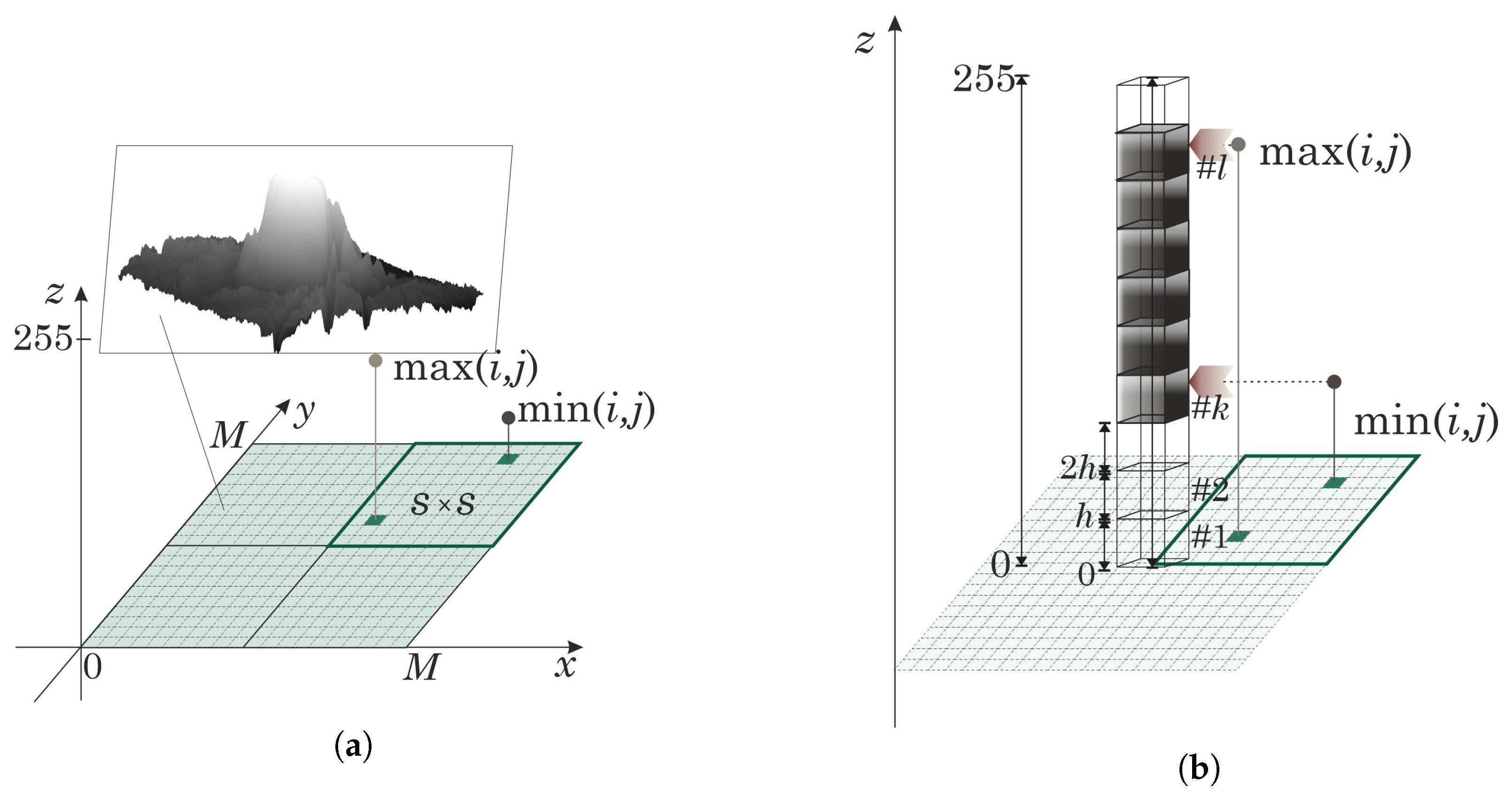
The differential box-counting method, originally proposed by [36], extends the box-counting concept to grayscale images by interpreting pixel intensity as a third dimension. A grayscale image of size $M\times M$ pixels is treated as a three-dimensional surface, where the coordinates $(x,y)$ define the spatial position of a pixel, and the z-coordinate corresponds to the pixel intensity value, ranging from 0 to $G-1$ (with $G=256$ for an 8-bit image). In this representation, the surface remains topologically two-dimensional but is embedded in ${\mathbb{R}}^3$, allowing its fractal dimension to range from 2 (perfectly smooth) to 3 (extremely rough). A schematic illustration of the DBC algorithm is provided in Figure 1.

The differential box-counting algorithm is implemented through the following steps.

Step 1. Scale selection. The image of size $M\times M$ pixels is partitioned into non-overlapping square grids of size $s\times s$ pixels, where s takes values such as 2, 4, 8, 16, 32, 64, $\dots ,M/2$. For each scale, the scaling factor is defined as $r=s/M$. The grid cells are indexed by $(i,j)$, where $i=1,\dots ,M/s$ and $j=1,\dots ,M/s$, with i and j denoting the row and column positions, respectively.

Step 2. Box height determination. To ensure scale invariance, the height h of each three-dimensional box is coupled to the grid size s:

$$h={\displaystyle \frac{s·G}{M}},$$

(9)

where $G=256$. This coupling preserves the proportion $h/s=G/M$, guaranteeing that the fractal dimension estimate is independent of image resolution.

Step 3. Intensity range within each cell. For each grid cell $(i,j)$, the minimum and maximum intensity values are identified:

$${\min }_{ij}=\min \{I(x,y):(x,y)\in \mathrm{cell}(i,j)\},{\max }_{ij}=\max \{I(x,y):(x,y)\in \mathrm{cell}(i,j)\}.$$

(10)

Step 4. Box indices for min and max. The entire intensity range $[0,G-1]$ is divided into vertical boxes (layers) of equal height h. The box indices for the minimum and maximum intensities are:

$$k=⌊{\displaystyle \frac{{\min }_{ij}}{h}}⌋+1,l=⌊{\displaystyle \frac{{\max }_{ij}}{h}}⌋+1,$$

(11)

where $\lfloor ·\rfloor$ denotes the floor function.

Step 5. Number of boxes covering the cell. The number of vertical boxes required to cover the intensity variation within cell $(i,j)$ is:

$$n_r(i,j)=l-k+1.$$

(12)

If the intensity surface is flat within the cell (${\min }_{ij}={\max }_{ij}$), then $l=k$ and $n_r(i,j)=1$.

Step 6. Total boxes for the entire image. Summing over all grid cells, the total number of boxes of size $s\times s\times h$ needed to cover the entire intensity surface at scale r is:

$$N_r=\sum _{i,j}{n}_r(i,j).$$

(13)

Step 7. Repetition across scales. Steps 1 through 6 are repeated for each selected grid size s, yielding a set of points $(\log (1/r),\log N_r)$.

Step 8. Fractal dimension estimation. The values of $\log N_r$ are plotted against $\log (1/r)$ in double logarithmic coordinates. A straight line is fitted to the points using the least squares method. The slope of this line is the fractal dimension $FD$:

$$\log N_r=FD·\log \left({\displaystyle \frac{1}{r}}\right)+C,$$

(14)

where C is the intercept.

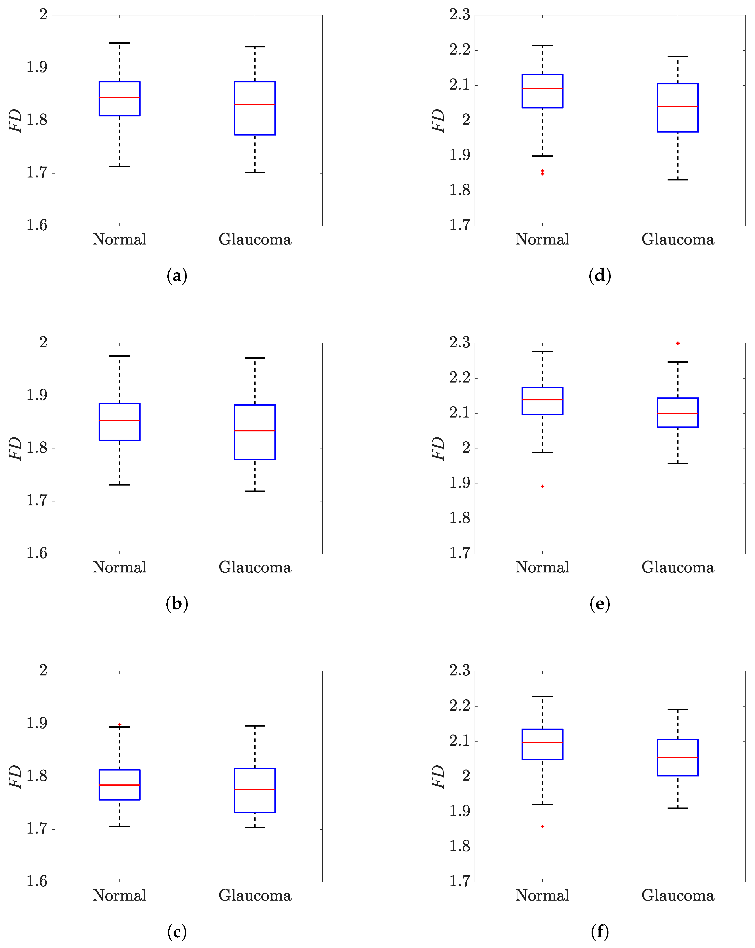
In this study, the differential box-counting method was applied to both the full retinal images and the extracted optic nerve head crops to obtain fractal dimension estimates for each image type.

For full retinal images and ONH crops (resized to 2048 × 2048), the grid sizes were s = 2, 4, 8, 16, 32, 64, 128, 256, 512, 1024. Partial boundary cells were included using their actual size (no discarding).

2.5. Multifractal Analysis

Unlike classical box-counting, which estimates structural complexity with a single number, multifractal analysis characterizes the heterogeneity and variability in a structure across different scales [17]. For objects with complex spatial organization, such as the retinal vascular network, the multifractal approach provides a more complete quantitative description since different regions may exhibit different local fractal properties.

Binary vessel masks of size $500\times 750$ pixels were partitioned into non-overlapping square boxes of size $L\times L$, where L took values from the set $\{2,3,5,10,25,50,100,125,250\}$ pixels. For each box $(i,j)$, a probability measure was calculated:

$$W_{ij}\left(L\right)={\displaystyle \frac{c_{ij}\left(L\right)}{{\sum }_{i,j}{c}_{ij}\left(L\right)}},$$

(15)

where $c_{ij}\left(L\right)$ is the number of vessel pixels in box $(i,j)$.

To characterize multifractal properties, a family of normalized measures parameterized by the moment order q was introduced:

$${\nu }_{ij}(q,L)={\displaystyle \frac{{\left[W_{ij}\left(L\right)\right]}^q}{{\sum }_{i,j}{\left[W_{ij}\left(L\right)\right]}^q}}.$$

(16)

The values of q ranged from $-1$ to 1 with a step of $0.05$.

For each q, the partition function was computed as follows:

$$Z(q,L)=\sum _{i,j}{\left[W_{ij}\left(L\right)\right]}^q.$$

(17)

The singularity exponent $\alpha \left(q\right)$ and the multifractal spectrum $f\left(q\right)$ were determined as the slopes of the linear regressions of $\sum {\nu }_{ij}(q,L)\ln W_{ij}\left(L\right)$ and $\sum {\nu }_{ij}(q,L)\ln {\nu }_{ij}(q,L)$ against $\ln L$, respectively. Only q values with a coefficient of determination $R^2>0.95$ were retained.

From the resulting singularity spectrum $f\left(\alpha \right)$, the following features were extracted for classification:

• Spectrum width $\Delta \alpha ={\alpha }_{\max }-{\alpha }_{\min }$, which characterizes the degree of structural heterogeneity;
• Singularity exponents ${\alpha }_{\min }$, ${\alpha }_{\max }$, and ${\alpha }_0$ (where $f\left({\alpha }_0\right)$ attains its maximum);
• Corresponding fractal dimensions $f\left({\alpha }_{\min }\right)$, $f\left({\alpha }_{\max }\right)$, and $f_{\max }=f\left({\alpha }_0\right)=D_0$.

2.6. Retinal Vessel Segmentation Using U-Net

Network Architecture, Preprocessing and Augmentation

Segmentation of the retinal vascular network using a neural network offers substantial advantages over classical morphological operators. In preliminary experiments, conventional methods (including matched filtering, morphological reconstruction, and thresholding) failed to reliably extract thin capillaries, directly compromising the accuracy of subsequent glaucoma diagnosis. Given that retinal vessels exhibit fractal-like branching patterns across multiple scales, preserving fine vascular structure during segmentation is critical for reliable fractal dimension estimates. Accurate vessel segmentation therefore serves as a prerequisite for reliable fractal dimension estimation via the differential box-counting method.

For vessel segmentation in fundus images, the U-Net convolutional architecture was adopted [27]. U-Net is particularly effective in biomedical segmentation tasks where training data is scarce, owing to its symmetric encoder–decoder structure with skip connections that preserve spatial information at multiple resolution levels. The network was implemented using MATLAB’s Deep Learning Toolbox. The encoder depth was set to four levels, balancing the receptive field against computational complexity. Input images were resized to $512\times 512$ pixels and converted to a single monochannel. The output produced a two-channel pixel-wise classification distinguishing vessels from background. The architecture of the U-Net neural network is shown in Figure 2.

All input images were originally in RGB format. Preprocessing involved extracting the green channel, which provides maximum contrast between vessels and the retinal background, followed by normalization to the double data type in the range $[0,1]$. To improve generalization, online data augmentation was applied prior to network feeding using the following transformations:

• Random rotation within $[-{30}^{°},+{30}^{°}]$ with bilinear interpolation for images and nearest-neighbor for ground truth masks;
• Random scaling by a factor in $[0.8,1.2]$ followed by cropping or resizing back to $512\times 512$ pixels;
• Random brightness and contrast adjustments with coefficients drawn uniformly from $[0.9,1.1]$;
• All images from the combined datasets were resized to 512 × 512 pixels while preserving the original aspect ratio. Padding (zero-padding) was applied to achieve the final square dimensions, ensuring that vascular structures were not distorted. The resizing was performed using bilinear interpolation for the fundus images and nearest-neighbour interpolation for the vessel masks to preserve binary label integrity.

2.7. Machine Learning Classification

The final stage consisted of binary classification of fundus images into healthy and glaucoma-diagnosed classes. Input features comprised numerical descriptors extracted in previous stages: fractal dimension computed via the differential box-counting (DBC) method, GLCM-based texture features for both full retinal images and the extracted optic nerve head (ONH) region, and multifractal characteristics of the vascular network. The total feature vector consisted of 18 descriptors: 5 GLCM features × 2 domains (full image and ONH crop) = 10 texture features, plus 1 DBC fractal dimension, 1 cup-to-disc ratio, and 6 multifractal parameters ($\Delta \alpha$, ${\alpha }_{\min }$, ${\alpha }_{\max }$, $f\left({\alpha }_{\min }\right)$, $f\left({\alpha }_{\max }\right)$, ${\alpha }_0$) from the vessel masks.

Two independent datasets were used for model development and validation. The training set contained feature vectors together with the binary class label. The test set was reserved for final evaluation and played no role in hyperparameter tuning. To select the optimal classifier, an automated pipeline was implemented comparing several algorithms using grid search with five-fold cross-validation and accuracy as the evaluation metric

Table 2. Hyperparameter grids used for grid search with 5-fold stratified cross-validation.

Model	Hyperparameter	Values (Grid)
Logistic Regression	C	0.001, 0.01, 0.1, 1, 10, 100, 1000
	l1_ratio	0, 0.5, 1
	solver	saga (only)
Random Forest	n_estimators	50, 100, 200, 300, 400, 500
	max_depth	5, 10, 20, None
	min_samples_split	2, 5, 10
	min_samples_leaf	1, 2, 4
	max_features	‘sqrt’, ‘log2’, None, 0.5
	bootstrap	True, False
	class_weight	None, ‘balanced’, ‘balanced_subsample’
SVM	C	0.01, 0.1, 1, 10, 100
	kernel	‘linear’, ‘poly’, ‘rbf’, ‘sigmoid’
	gamma	‘scale’, ‘auto’, 0.001, 0.01, 0.1
	degree (for poly)	2, 3, 4, 5
	probability	True, False
	class_weight	None, ‘balanced’
Gradient Boosting	n_estimators	50, 100, 200, 300, 500
	learning_rate	0.001, 0.01, 0.1, 0.2
	max_depth	3, 5, 7, 9
	min_samples_split	2, 5, 10
	min_samples_leaf	1, 2, 4
	subsample	0.8, 0.9, 1.0
	max_features	‘sqrt’, ‘log2’, None
k-NN	n_neighbors	3, 5, 7, 9, 11, 15
	weights	‘uniform’, ‘distance’
	algorithm	‘auto’, ‘ball_tree’, ‘kd_tree’, ‘brute’
	leaf_size	20, 30, 40, 50
	p	1, 2
	metric	‘euclidean’, ‘manhattan’, ‘minkowski’
Time Series Forest	n_estimators	50, 100, 200
	min_window_size	0.1, 0.3, 0.5
	n_windows	10, 20, 30
	n_jobs	−1, 1, 2, 4
	random_state	None, 42
	criterion	‘gini’, ‘entropy’
	min_samples_split	2, 5, 10
	min_samples_leaf	1, 3, 5
	max_features	‘sqrt’, ‘log2’

. The following models were tested: logistic regression, Random Forest, Support Vector Machine (SVM), Gradient Boosting, k-Nearest Neighbors (kNN), and Time Series Forest. A dedicated hyperparameter space was defined for each model, and the configuration maximizing cross-validated accuracy was selected for final evaluation.

After training, the models were evaluated on the held-out test set using accuracy, area under the ROC curve (AUC-ROC), average precision (AP) from the precision–recall curve, and the $F_1$-score metrics. For the Random Forest and Gradient Boosting models, feature importance analysis was performed based on the mean decrease in impurity averaged over all trees. The resulting values were normalized to sum to one, revealing the most discriminative characteristics for glaucoma diagnosis.

After selecting the best model based on cross-validation, a final evaluation was conducted on the independent test set. For every test image, the predicted probability of belonging to the glaucoma class was computed along with the binary label obtained using the optimal probability threshold. The number of misclassifications was recorded as an estimate of the model’s generalization ability.

Grid search was performed using stratified 5-fold cross-validation (preserving class distribution). The random seed was fixed at 42 for reproducibility. The best model was selected based on the highest cross-validation accuracy.

2.8. Evaluation Metrics and Model Analysis

After training, the models were evaluated on the held-out test set using accuracy, area under the ROC curve (AUC-ROC), average precision (AP) from the precision–recall curve, and the $F_1$-score. Accuracy was defined as follows:

$$\mathrm{Accuracy}={\displaystyle \frac{TP+TN}{TP+TN+FP+FN}}$$

where $TP$ (true positives) and $TN$ (true negatives) are correctly classified vessel and background pixels, $FP$ (false positives) are background pixels incorrectly classified as vessels, and $FN$ (false negatives) are vessel pixels missed by the model.

The $F_1$-score, representing the harmonic mean of precision and recall, was computed as follows:

$$F_1=2·{\displaystyle \frac{\mathrm{Precision}·\mathrm{Recall}}{\mathrm{Precision}+\mathrm{Recall}}}$$

For the Random Forest and Gradient Boosting models, feature importance was derived from the mean decrease in impurity averaged over all trees in the ensemble. The obtained values were normalized to sum to one, which allowed for ranking the features by their contribution to the classification and identifying the most informative characteristics for glaucoma diagnosis.

The best model selected from cross-validation underwent final testing on the independent test set. For each test image, the predicted probability of belonging to the glaucoma class was computed together with the final binary label obtained using the optimal probability threshold. The number of misclassifications was recorded to assess the model’s generalization ability.

3. Results and Discussion

3.1. Retinal Vessel Segmentation

A U-Net neural network was trained for vessel segmentation using the public datasets listed in Table 1. Visual inspection of the segmentation results on test images confirmed that the model successfully delineated both large vessels and thin capillaries, including regions with low contrast. Figure 3 shows representative segmentation examples. The resulting binary vessel masks served as input for subsequent multifractal analysis.

3.2. Textural Feature Extraction

For both full retinal images and optic nerve head crops, GLCM-based texture features were computed. Conversion to monochrome was performed using three methods: the standard weighted transformation in MATLAB (im2gray), averaging of the green and blue channels (AvrGB), and averaging of all three RGB channels (AvrRGB). For each method, five texture features were extracted: contrast, correlation, energy, homogeneity, and entropy. To assess statistical significance, p-values were calculated. Mean feature values for full retinal images and optic nerve head crops (ONH) are presented in

Table 3. Mean textural feature values for full retinal images.

	Contrast	Correlation	Energy	Homogeneity	Entropy
Normal (standard function)	0.012	0.99	0.39	0.99	1.67
Glaucoma (standard function)	0.010	0.99	0.43	0.99	1.57
Normal (AvrGB)	0.014	0.98	0.47	0.99	1.51
Glaucoma (AvrGB)	0.012	0.99	0.51	0.99	1.41
Normal (AvrRGB)	0.013	0.99	0.38	0.99	1.75
Glaucoma (AvrRGB)	0.011	0.99	0.39	0.99	1.69

and 

Table 4. Mean textural feature values for optic nerve head crops.

	Contrast	Correlation	Energy	Homogeneity	Entropy
Normal (standard function)	0.005	0.99	0.36	0.99	1.70
Glaucoma (standard function)	0.005	0.99	0.35	0.99	1.74
Normal (AvrGB)	0.007	0.99	0.28	0.99	2.09
Glaucoma (AvrGB)	0.006	0.99	0.26	0.99	2.14
Normal (AvrRGB)	0.004	0.99	0.36	0.99	1.72
Glaucoma (AvrRGB)	0.004	0.99	0.33	0.99	1.78

, respectively.

For all three conversion methods, all five texture features showed statistically significant differences between the normal and glaucoma groups. The lowest p-values were obtained for the RGB averaging method: contrast ($7.55\times {10}^{-6}$), correlation ($4.84\times {10}^{-4}$), energy ($0.0036$), homogeneity ($7.61\times {10}^{-6}$), and entropy ($0.0025$). In the glaucoma group, contrast, correlation, homogeneity, and entropy decreased, while energy increased relative to the normal group.

For ONH crops, statistically significant differences were identified for correlation, energy, and entropy. The most pronounced differences were observed for the standard green channel extraction (im2gray): correlation ($6.49\times {10}^{-5}$), energy ($5.50\times {10}^{-4}$), and entropy ($0.0052$). Contrast and homogeneity did not reach statistical significance ($p>0.05$) for any conversion method. These results indicate that textural changes in glaucoma are most informatively reflected in contrast, energy, and entropy, with the nature of these changes differing between full retinal images and ONH crops.

3.3. Fractal and Multifractal Analysis

Fractal dimension was computed using the differential box-counting method for both ONH crops and full retinal images, applying the three monochrome conversion methods described in Section 2.2.

Table 5. Mean fractal dimension values computed using the differential box-counting method for ONH crops and full retinal images.

Image Type	Conversion Method	Normal	Glaucoma
ONH crops	standard function (im2gray)	1.84	1.82
	AvrGB	1.85	1.83
	AvrRGB	1.79	1.77
Full retinal images	standard function (im2gray)	2.08	2.03
	AvrGB	2.13	2.09
	AvrRGB	2.09	2.05

presents the mean fractal dimension values. In all cases, the glaucoma group showed a slight decrease in fractal dimension compared to the normal group: approximately 0.02 for ONH crops and 0.04–0.05 for full retinal images, corresponding to a relative change of 1–2%. Despite the small absolute magnitude, this trend was consistent across all conversion methods and image types. Figure 4 shows the fractal dimension distributions for ONH crops and full retinal images.

Statistical comparison of fractal dimension between healthy and glaucomatous groups was performed using the two-tailed Mann–Whitney U test. For ONH crops, all three grayscale conversion methods yielded statistically significant differences: p = 0.0115 (im2gray), p = 0.0043 (AvrGB), and p = 0.0193 (AvrRGB). For full retinal images, the differences were even more pronounced: p = 9.94 × 10⁻⁹ (im2gray), p = 1.63 × 10⁻⁸ (AvrGB), and p = 2.54 × 10⁻⁸ (AvrRGB). Despite these low p-values, the absolute differences in fractal dimension between groups are very small (≈0.02 for ONH crops and ≈0.04–0.05 for full retinal images, corresponding to relative changes of only 1–2%). The distributions overlap substantially (Figure 4), indicating that classical fractal dimension lacks practical discriminatory power for individual diagnosis. In contrast, multifractal parameters show much larger relative changes (up to 15% for $\Delta \alpha$) and are far more sensitive to glaucomatous alterations.

Unlike fractal dimension, multifractal analysis characterizes the heterogeneity of vascular element distribution. This analysis was performed on binary vessel masks obtained from U-Net segmentation.

Table 6. Mean multifractal parameters extracted from the singularity spectrum.

Parameter	Normal	Glaucoma	Relative Change
$\Delta \alpha$	0.439	0.507	15%
${\alpha }_{max}$	1.481	1.410	5%
${\alpha }_{min}$	1.042	0.903	13%
$f\left({\alpha }_{max}\right)$	1.645	1.587	4%
$f\left({\alpha }_{min}\right)$	1.461	1.425	2%
${\alpha }_0$	1.414	1.282	9%

presents the multifractal parameters extracted from the singularity spectrum. The most pronounced differences between groups were observed for the spectrum width $\Delta \alpha$ (relative change of 15%), the minimum singularity exponent ${\alpha }_{min}$ (13%), and ${\alpha }_0$ (9%). In the glaucoma group, $\Delta \alpha$ increased from $0.439$ to $0.507$, indicating widening of the multifractal spectrum. This increase in heterogeneity of vascular element distribution may reflect microcirculatory remodeling in glaucoma.

Figure 5 presents the averaged multifractal singularity spectra for the normal and glaucoma groups. In the glaucoma group, the spectrum shifted toward lower singularity exponent values, confirming altered vascular network heterogeneity under pathological conditions. Multifractal parameters demonstrated higher sensitivity to pathological changes than classical fractal dimension.

From a pathophysiological perspective, the observed increase in the multifractal spectrum width $\Delta \alpha$ and the decrease in the minimum singularity exponent ${\alpha }_{\min }$ in glaucomatous eyes are consistent with progressive microvascular rarefaction and remodeling of the retinal capillary network. Glaucoma is known to involve not only structural damage to the optic nerve head but also chronic ischemia and impaired autoregulation of retinal blood flow. The widening of the multifractal spectrum indicates greater spatial heterogeneity in the distribution of vessel diameters and branching patterns, which may reflect focal capillary dropout, vessel tortuosity, and altered fractal scaling of the microvasculature. The shift in the spectrum toward lower $\alpha$ values suggests an increased proportion of regions with sparse or disconnected vascular elements, consistent with the loss of fine capillaries in the peripapillary area. These microvascular changes are clinically relevant because they may precede visible optic disc excavation and could serve as early biomarkers of glaucomatous damage, especially in patients with normal-tension glaucoma where conventional CDR assessment is often inconclusive.

3.4. Machine Learning Classification Results

Unlike end-to-end neural networks, which often operate as black boxes, the feature-based machine learning approach enables interpretation of the decision-making process. This transparency is critical for potential clinical application. Model training was performed independently for two scenarios differing in input data type. In the first scenario, features were derived from two types of monochrome images: ONH crops and full retinal images. For each of these two image types, three alternative grayscale conversion methods were applied: the standard weighted transformation (im2gray), averaging of the green and blue channels (AvrGB), and averaging of all three RGB channels (AvrRGB). Thus, an independent feature set was formed for each combination of image type and conversion method. The feature vector for each variant comprised the fractal dimension computed via the differential box-counting (DBC) method, five GLCM texture features (contrast, correlation, energy, homogeneity, entropy), and the cup-to-disc ratio. In the second scenario, features were derived from binary vessel masks obtained after U-Net segmentation. The feature vector comprised six multifractal parameters extracted from the singularity spectrum ($\Delta \alpha$, ${\alpha }_{\min }$, ${\alpha }_{\max }$, $f\left({\alpha }_{\min }\right)$, $f\left({\alpha }_{\max }\right)$, ${\alpha }_0$) together with the cup-to-disc ratio. Models using only CDR were trained as a baseline for both scenarios.

For each scenario, the following algorithms were tested: logistic regression, Support Vector Machine, Random Forest, Gradient Boosting, k-Nearest Neighbors, and Time Series Forest. Hyperparameter optimization was performed using grid search with five-fold cross-validation. The Random Forest model on ONH crops reached 75.00% accuracy (AUC = 0.778), while the logistic regression model on multifractal features + CDR yielded 86.17% (AUC = 0.893). The corresponding sensitivity and specificity on the test set were 59.26% and 80.52%, respectively. For comparison, the model trained on CDR alone achieved 66.15% accuracy, confirming the value of additional textural and fractal features.

Among the six classifiers evaluated (logistic regression, Random Forest, SVM, Gradient Boosting, k-NN, and Time Series Forest), Random Forest and logistic regression consistently outperformed the other models across both feature sets. We therefore focused our detailed analysis on these two best-performing models.

Figure 6 presents the correlation heatmap for all features. CDR showed the highest correlation with the glaucoma diagnosis (0.53), consistent with clinical evidence. Other features showed weaker correlations: fractal dimension ($-0.10$), texture correlation ($0.16$), and energy ($-0.12$). These low correlations explain why CDR-only models achieved only 66.15% accuracy, while incorporating additional features improved performance to 75.00% by leveraging information not overlapping with CDR.

Feature importance analysis for the Random Forest model (Figure 7) revealed that CDR made the largest contribution (importance 0.466), consistent with its clinical role. Fractal dimension (importance 0.115) and texture correlation (importance 0.104) also contributed substantially, exceeding the average importance of remaining texture features (energy, contrast, entropy, and homogeneity), which was 0.079. These results confirm that while CDR dominates, fractal and textural characteristics provide complementary diagnostic information, explaining the accuracy improvement when used together.

For binary vessel masks analyzed using multifractal parameters together with CDR, the logistic regression model achieved an accuracy of 86.17% on the same test set.

Table 7. Classification performance on the test set.

Model	Acc. (%)	Sen. (%)	Spe. (%)	F1-Score (%)	AUC
Random Forest (ONH crops)	75.00	59.26	80.52	55.17	0.778
Logistic Regression (multifractal + CDR)	86.17	59.26	97.01	71.11	0.893

and Figure 8 summarize the full set of classification metrics and ROC curves for both models. This performance was higher than that for ONH crops (75.00%) and higher than CDR alone (66.15%). This may reflect that multifractal parameters, despite their sensitivity to structural changes (Section 3.3), correlate less strongly with traditional clinical indicators.

Figure 9 presents the correlation matrix for CDR and multifractal parameters. CDR again showed the highest correlation with the target variable (0.58). Multifractal parameters showed lower correlations: $\Delta \alpha$ ($-0.18$), ${\alpha }_{max}$ ($-0.39$), ${\alpha }_{min}$ ($-0.28$), $f\left({\alpha }_{max}\right)$ ($-0.37$), $f\left({\alpha }_{min}\right)$ ($-0.42$), ${\alpha }_0$ ($-0.42$). Notably, CDR exhibited weak correlation with multifractal features, indicating complementarity. This complementarity explains why combining feature types improves classification accuracy compared to using CDR alone.

To provide a clinically oriented evaluation, Table 7 reports accuracy, sensitivity, specificity, F1-score, and AUC for the proposed Random Forest model using ONH crop features and the logistic regression model using multifractal parameters from vessel masks combined with CDR. The Random Forest model achieves a sensitivity of 59.26%, a specificity of 80.52%, and an AUC of 0.778, while the logistic regression model yields higher specificity (97.01%) and AUC (0.893).

4. Conclusions

Classical fractal dimension alone does not adequately indicate the complexity of glaucomatous vascular changes. Thus, this study demonstrates that the diagnostic information carried by the retinal vascular network is predominantly multifractal in nature. While the differential box-counting method yielded only marginal differences between healthy and glaucomatous eyes—approximately 0.02 for optic nerve head crops and 0.04–0.05 for full retinal images, corresponding to relative changes of 1–2% with substantial overlap between groups—multifractal analysis of binary vessel masks obtained from U-Net segmentation revealed pronounced and consistent differences. The width of the multifractal spectrum $\Delta \alpha$ changed by 15%, the minimum singularity exponent ${\alpha }_{\min }$ by 13%, and ${\alpha }_0$ by 9%, with the glaucoma group showing a wider spectrum and a shift toward lower singularity exponents.

The observed changes are consistent with increased heterogeneity of the microvascular bed in glaucoma, likely reflecting microvascular remodeling and altered capillary organization. When used for classification, the cup-to-disc ratio alone achieved 66.15% accuracy. Adding fractal and textural features from optic nerve head crops improved accuracy to 75.00% with a Random Forest classifier. Using multifractal parameters from segmented vessel masks together with the cup-to-disc ratio yielded 86.17% accuracy with logistic regression. Feature importance analysis confirmed that while the cup-to-disc ratio remains the strongest single predictor, fractal and multifractal features contribute complementary information not correlated with the cup-to-disc ratio.

Overall, multifractal spectrum parameters provide a more sensitive description of glaucomatous vascular changes than classical fractal dimension. Their combination with texture features and the cup-to-disc ratio offers an interpretable machine learning framework for glaucoma screening, with potential applications in other retinal diseases involving the microvasculature.

Despite the promising results, several limitations should be acknowledged. First, this study was conducted on a single public dataset (ORIGA) with a limited number of glaucoma cases. The generalizability of the proposed method to other populations, imaging devices, or ethnic groups remains to be verified. Future work will include external validation on independent datasets.

Second, the ORIGA dataset does not provide staging information for glaucoma severity (early, moderate, advanced). The diagnostic performance of the proposed features may differ across disease stages, particularly in early glaucoma where vascular changes are subtle. Subsequent studies should evaluate the method on stratified cohorts with clinical severity labels to assess stage-specific sensitivity.

Third, image quality and variability (e.g., uneven illumination, motion artefacts, media opacities) were not explicitly controlled for in this study. Such factors can affect both vessel segmentation and texture extraction. In future work, we plan to incorporate automated quality assessment and preprocessing steps tailored to low-quality fundus images.