Pruning Policy for Image Classification Problems Based on Deep Learning

Abstract

In recent years, several methods have emerged for compressing image classification models using CNNs, for example, by applying pruning to the convolutional layers of the network. Typically, each pruning method uses a type of pruning distribution that is not necessarily the most appropriate for a given classification problem. Therefore, this paper proposes a methodology to select the best pruning policy (method + pruning distribution) for a specific classification problem and global pruning rate to obtain the best performance of the compressed model. This methodology was applied to several image datasets to show the influence not only of the method but also of the pruning distribution on the quality of the pruned model. It was shown that the selected pruning policy affects the performance of the pruned model to different extents, and that it depends on the classification problem to be addressed. For example, while for the Date Fruit Dataset, variations of more than 10% were obtained, for CIFAR10, variations were less than 5% for the same cases evaluated.

1. Introduction

Deep learning (DL) is one of the most widely used branches of artificial intelligence in image processing tasks, such as classification, detection, and segmentation. Multiple DL models have been trained in the literature with millions of images, learning different types of features, such as geometric and spatial features, obtaining trained models such as VGG-16 [1] and ResNet, with high classification performance values [2]. As a result, several trained models have been used as a backbone in image recognition applications. Specifically, in the field of agriculture, they are used in harvesting [3], storage [4], fruit detection [5], and disease and weed control tasks [6,7]. However, when we want to use this type of model in portable or low-cost devices, we face the challenge of high computational costs, due to the elevated number of floating-point operations (FLOPs) needed to perform the predictions.

As a consequence, it is relevant to apply DL model compression techniques in order to have solutions in industries such as agriculture that are not only successful in terms of classification but also efficient in terms of resource management [8]. In state-of-the-art compression methods, DL models, especially convolutional neural networks (CNNs), are compressed using different techniques such as quantization, low-rank factorization, separable convolution, and knowledge distillation [9,10]. Among them, the most popular is known as pruning, in which weights are discarded or removed from the network to make it smaller and faster, ideally with little impact on model performance [11,12].

Pruning methods started to be applied in artificial intelligence to models that are composed of multiple weights/neurons, especially multi-layered perceptrons [13,14,15]. Some of them were applied during the training of the model. For example, in the calculation of the sensitivity of the weights, removing those weights at the end of the training obtains the lowest value [13,16]. Anther pruning method is the use of penalty factors that remove the weight, setting it to a value of zero [13]. However, the disadvantage of these methods is that some weights are evaluated independently, without correlating their importance combined with other weights, or they can remove weights at the beginning of the training that can be of importance later in the training. Another proposal is a post-training pruning method for feedforward networks that iteratively removes non-significant weights and then fine-tunes the remaining ones [16].

In some areas of Industry 4.0, such as agriculture, pruning methods have been used to overcome the problems of computational cost and long inference times of networks. For example, separable convolutions have been used together with a fixed pruning scheme to compress a disease classification model of multiple crop types [17]. Pruning (specifically L2-norm) has also been combined with quantization for seed recognition of plants [9], where only the convolutional layers are uniformly pruned, i.e., with the same pruning rate (PR) in each layer. A similar approach was used in [18] to detect weeds in plant leaves. On the other hand, pruning methods are also very attractive for agricultural detection tasks, especially with the YOLO architecture [19,20,21].

But what policy is taken into account when pruning a model? First, the criteria for selecting the parameters to be pruned, i.e., the pruning method, are considered. Second is the pruning distribution (PD), which consists of selecting the pruning rate (PR) per layer. It can be uniform (i.e., the same PR for all layers) or variable by layer (e.g., top-down or bottom-up). Third (optional) is if you want to restructure the network or simply reset the pruned parameters to zero (default). Regarding the criteria for pruning parameters, there are methods based on the size of the weights [9,22], the size of the gradients associated with the network during the training process [23,24], using Taylor expansion to estimate the importance of the weights [25,26], reinforcement learning [27], and those based on the importance of the weights for each class [28]. On the other hand, the parameters to be pruned can be set to zero, and sparse algebra libraries can be used to reduce inference times [29], or architectural restructuring techniques can be implemented [30,31,32]. Although the CNN pruning criterion has typically been the most researched pruning policy, PD (e.g., bottom-up, top-down, uniform) may have a greater impact on classifier performance. Some studies have applied a uniform PD [28], i.e., the same PR in each convolutional layer, but others have used another type of PD, e.g., a high value at the beginning of the network and lower values for the end [33,34], as well as the opposite way [35]. On the other hand, several techniques have been used to identify the most suitable PD, e.g., k-means together with an optimization algorithm called SGO, to facilitate the model compression process [36], or reinforcement learning to automatically determine the optimal pruning rate for each convolutional layer [35].

However, there is no consolidated view on the state-of-the-art pruning policy for CNNs, which would allow us to select the best distribution and pruning method pair. To date, studies that have evaluated the impact of PD have only compared one distribution per method (not necessarily the best), leading to biased conclusions.

In consideration of the above, the contributions of this study are as follows:

• We propose the following methodology to evaluate the impact of the pruning policy on a given classification problem (dataset): consider the impact of the pruning method regardless of the pruning distribution used, consider impact of the pruning distribution regardless of the pruning method used, and select the best pruning policy from a set of choices generated with different pruning methods and distribution types.
• From the case studies used in the application of the proposed methodology, it was possible to disprove the belief that the worst pruning distribution is the homogeneous one, given that, in several contexts, it was even better than its competitors.
• In addition, it should be noted that the pruning policy does not have the same effect on all image classification problems. For example, when using CIFAR10, the differences in accuracy between a good and a less good pruning policy can be less than 5%, while for the Date Fruit Dataset, the differences can be more than 10% for the same cases evaluated.

2. Preliminary Concepts

In this section, we explain some concepts related to deep learning, specifically CNNs and CNN pruning.

2.1. Convolutional Neural Networks

Convolutional networks (CNNs) are one of the fundamental techniques in deep learning, characterized by their efficiency in extracting patterns from images, as shown in several studies [37]. These architectures consist of several processing layers that progressively decompose features from different levels: from basic features to higher-level representations [38]. CNNs typically consist of convolutional layers, which actually perform cross-correlation [39]; fully connected (FC) layers, which can be interpreted as a traditional neural network or 1 × 1 convolutional layers; and finally an output layer (see Figure 1).

While CNNs have demonstrated exceptional performance in image-related tasks, many of the benchmark models involve millions or even hundreds of millions of parameters [41]. As a result, inference times can be very long, depending on the hardware on which they are implemented [42]. So what is causing the increase in inference times? At first glance, it might seem that the number of parameters plays a crucial role, but in fact, it depends largely on the type of operations performed by the network. For example, convolutional layers may have fewer parameters than fully connected (FC) layers, but they contribute more to the total number of floating-point operations (FLOPs). In this sense, inference times increase proportionally as the number of FLOPs increases [28].

The way the number of FLOPs is calculated varies depending on the type of layer. The following equations describe how this calculation is performed for each of the CNN layers, convolutional layers (conv), pooling layers (pool), and fully connected (FC) layers, as follows [28]:

$$FLOP{s}_{conv}=2\times (W_k\times H_k\times C_k)\times (W_o\times H_o)\times filters,$$

(1)

where $W_k$, $H_k$, and $C_k$ correspond to the width, height, and number of channels of the filter; $W_o$ and $H_o$ are the width and height of the output (feature map); and $filters$ is the number of filters of the current layer.

$$FLOP{s}_{F{C}^l}=2\times (neuron{s}^{l-1}\times neuron{s}^l),$$

(2)

where l is the current layer, $l-1$ is the previous layer, and $neurons$ is the number of neurons.

$$FLOP{s}_{poo{l}^l}=(W_o/S)\times (H_o/S)\times \left(filter{s}^{l-1}\right),$$

(3)

where S is the stride of the pooling operation.

On the other hand, the number of parameters are calculated, according to

$$Parameter{s}_{conv}=filters\times (W_k\times H_k\times C_k)+filters,$$

(4)

$$Parameter{s}_{F{C}^l}=(filter{s}^{l-1}\times filter{s}^l)+filter{s}^l),$$

(5)

It is noted that no parameters are generated in the pooling layers, only FLOPs.

2.2. Pruning Policy

Pruning is a strategy used to compress deep learning models and thus contributes to the reduction in inference times, without significantly affecting model performance. The pruning policy includes three parts: (1) criteria of the parameters to be pruned, i.e., pruning method, (2) pruning distribution, and optionally (3) network restructuring or zeroing of the pruned parameters. Each of these is explained below.

2.2.1. Criteria of the Parameters to Be Pruned

This is the first step in designing your model’s pruning policy. The purpose is to identify parameters that contribute little to the performance of the classifier and that can be removed or ignored from the network. There are several strategies for identifying these parameters, e.g., removing specific parameters from a channel and a filter (element-wise), removing channels from filters (channel-wise), removing the same element in all channels of a filter (shape-wise), removing filters (filter-wise), or completely removing a layer from the architecture (layer-wise) [11]. The element-wise and shape-wise types of unstructured pruning usually rely heavily on sparse algebra libraries to reduce inference times. While the other strategies correspond to structured pruning. However, filter-wise allows for greater parameter reduction than unstructured pruning while largely maintaining model accuracy, and does not require sparse algebra libraries to make decisions [29].

Among the various methods for selecting the parameters to be pruned, the following can be found in the literature:

• Random: in this case, the filters to be pruned in the convolutional layers are selected randomly.
• Weight: this pruning method is based on the estimation of the importance of the layer’s filters according to their weights. In this method, the L2-norm is calculated in each filter, and the ones with the highest values are kept [30]. This is because in CNNs, the filters at each layer with higher activation maps are assumed to be more important for the performance of the network. In this case, there is no required to use random seeds because Weight is a deterministic method, i.e., it is expected to obtain the same result under the same conditions.
• SeNPIS-Faster: SeNPIS is based on class-wise importance score calculation, which includes a class-wise importance score, class-wise importance score attenuation, and overall importance score [28]. In the case of SeNPIS-Faster, the stage responsible for performing the class-wise importance score attenuation is eliminated in order to significantly reduce the computational cost of applying pruning, with a very small decrease in accuracy (less than 0.5%) compared to SeNPIS [43].

2.2.2. Pruning Distribution (PD)

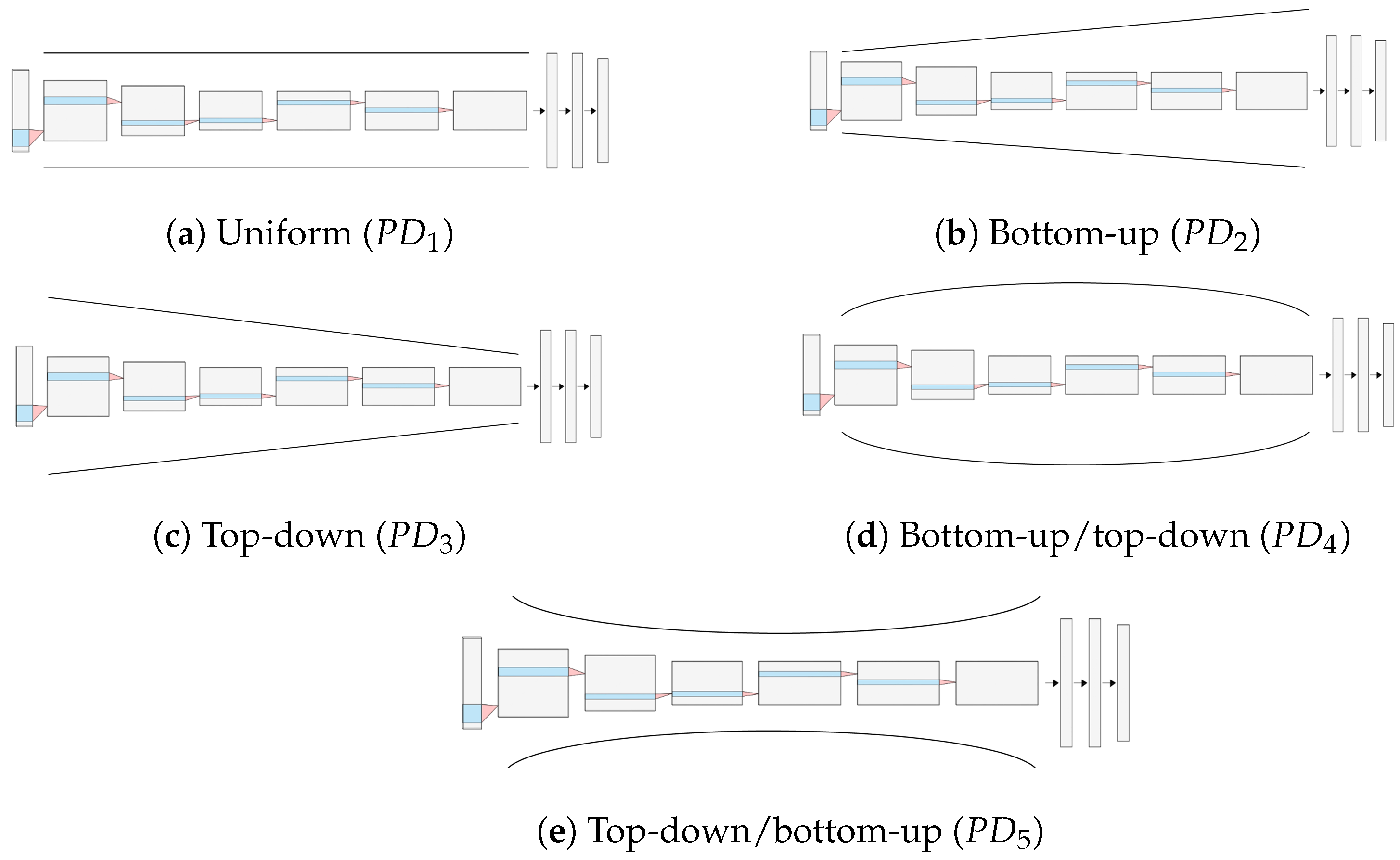
In this step, the objective is to apply the selection criteria of the parameters to be pruned for each of the convolutional (and even fully connected) layers, according to a pruning rate (PR) per layer. This value can be the same between convolutional layers if uniform pruning is used, or variable between layers if another distribution type such as bottom-up/top-down is used. This study includes five pruning distributions: uniform ($P{D}_1$), bottom-up ($P{D}_2$), top-down ($P{D}_3$), bottom-up/top-down ($P{D}_4$), and top-down/bottom-up ($P{D}_5$) (see Figure 2).

2.2.3. Network Restructuring or Zeroing of the Pruned Parameters

Figure 3 shows an example of the pruning process of a CNN. First, the layer to be pruned is selected, which contains N filters (e.g., six filters: $F_1$ to $F_6$). In the second step, a pruning method (e.g., L2-norm) is applied according to the PR (pruning rate) of the layer. For example, if the PR is 50%, half of the filters are pruned (e.g., $F_1$, $F_3$, and $F_5$).

These pruned filters can be treated in two ways: they can be converted to zeros or they can be removed from the network (network restructuring). In the first case, there is no real reduction in the FLOPs of the model, so it is necessary to use sparse algebra libraries for their computation. In the second case, the network is updated by modifying the filter size per layer and the filter channels of the next layer, as explained in [31]. Network restructuring reduces the number of FLOPs in the pruned model.

3. Methodology

Figure 4 shows the proposed methodology for selecting a pruning policy (including only the first two steps) for a given classification problem (i.e., a model trained on a given dataset).

This methodology includes the following phases: (1) dataset selection, (2) model training, (3) selection of pruning hyperparameters, including the global pruning rate (GPR), the PD, and the pruning method, (4) model pruning and fine-tuning, and (5) policy selection. It is worth mentioning that in the experimental phase, some pruning methods, GPR values, and distribution types were used, but the user can include other methods, more GPR values, and other distribution types than those used.

3.1. Dataset

The first step of the methodology is to select the dataset for the classification problem. For our experiments, we applied the methodology to two case studies: an agricultural dataset and a benchmark dataset.

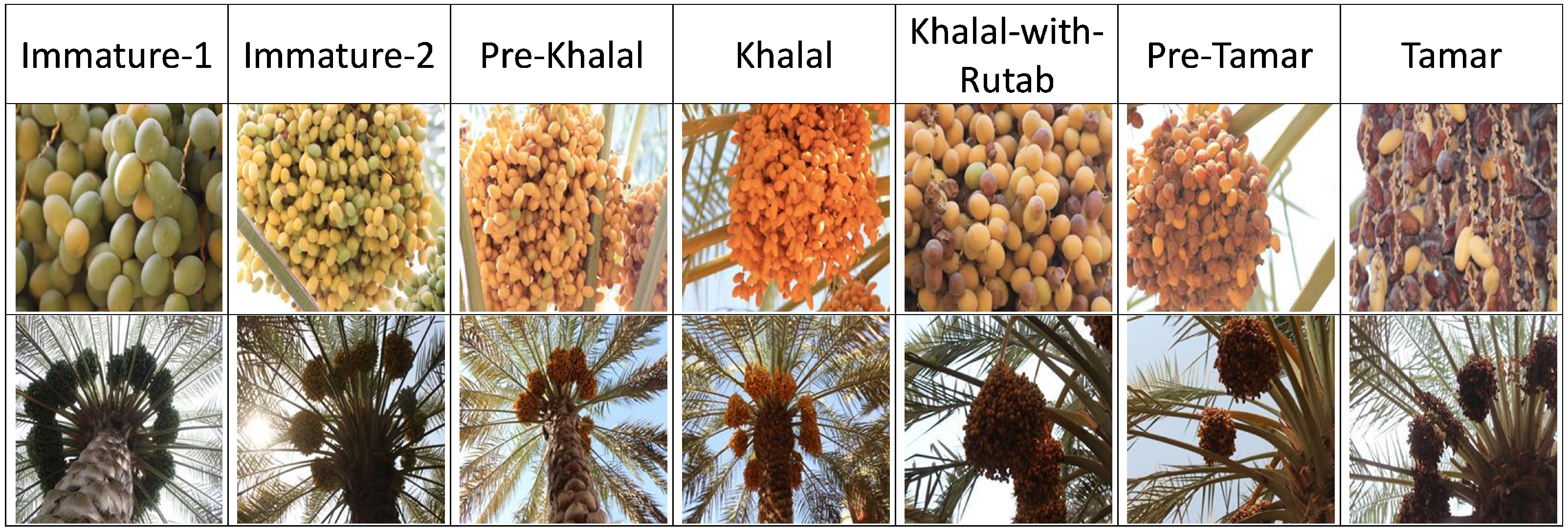
For the first case study, we used the Date Fruit Dataset [44], which is a public dataset used for date fruit harvesting developments. The dataset consists of images of date bunches of five species on different palm trees in a natural orchard environment. The images were captured by two cameras at different angles, daylight conditions, and distances from palm trees. They were also resized to 224 × 224 pixels in RGB format. For the experiments, it was decided to classify the maturity stages of the date fruits, i.e., into seven categories (Immature-1, Immature-2, Pre-Khalalal, Khalalal, Khalal-with-Rutab, Pre-Tamar, and Tamar), and divide them into training and test sets as described in [3]. A total of 3227 images were used for training (461 images per maturity stage) and 3420 for testing. It can be seen in Figure 5 that the images are not only of the fruit, but can also include part of the palm and the bunches, making the classification task more difficult.

The second case study uses a benchmark dataset called CIFAR10 [45]. The dataset comprises ten distinct classes: airplane, automobile, bird, cat, deer, dog, frog, horse, ship, and truck. Within each class, there are a total of six thousand color images, each of size of 32 × 32 pixels. This dataset is partitioned by default into fifty thousand images for training and an additional ten thousand images for testing purposes.

3.2. Model Training

In this second stage, a network is trained to obtain the unpruned model. For this study, VGG16 was selected because it is one of the most versatile networks with the largest number of parameters (more than 100 million) in the literature, and has been used in several image classification problems.

Table 1. Network and parameters of VGG-16. ($W_k$, $H_k$, $C_k$) is the width, height, and number of filter channels (k); ($W_o$, $H_o$, $C_o$) is the width, height, and channels of the output shape. This example has an output of 10 classes (as in CIFAR10).

Layer	Filters or Neurons	Filter Shape	Output Shape	Parameters	FLOPs
	$\mathit{k}$	$({\mathit{W}}_{\mathit{k}}$, ${\mathit{H}}_{\mathit{k}}$, ${\mathit{C}}_{\mathit{k}})$	$({\mathit{W}}_{\mathit{o}}$, ${\mathit{H}}_{\mathit{o}}$, ${\mathit{C}}_{\mathit{o}})$
$block1conv1$	64	(3, 3, 3)	(224, 224, 64)	1792	173,408,256
$block1conv2$	64	(3, 3, 64)	(224, 224, 64)	36,928	3,699,376,128
$block1pool$	–	–	(112, 112, 64)	0	802,816
$block2conv1$	128	(3, 3, 64)	(112, 112, 128)	73,856	1,849,688,064
$block2conv2$	128	(3, 3, 128)	(112, 112, 128)	147,584	3,699,376,128
$block2pool$	–	–	(56, 56, 128)	0	401,408
$block3conv1$	256	(3, 3, 128)	(56, 56, 256)	295,168	1,849,688,064
$block3conv2$	256	(3, 3, 256)	(56, 56, 256)	590,080	3,699,376,128
$block3conv3$	256	(3, 3, 256)	(56, 56, 256)	590,080	3,699,376,128
$block3pool$	–	–	(28, 28, 256)	0	200,704
$block4conv1$	512	(3, 3, 256)	(28, 28, 512)	1,180,160	1,849,688,064
$block4conv2$	512	(3, 3, 512)	(28, 28, 512)	2,359,808	3,699,376,128
$block4conv3$	512	(3, 3, 512)	(28, 28, 512)	2,359,808	3,699,376,128
$block4pool$	–	–	(14, 14, 512)	0	100,352
$block5conv1$	512	(3, 3, 512)	(14, 14, 512)	2,359,808	924,844,032
$block5conv2$	512	(3, 3, 512)	(14, 14, 512)	2,359,808	924,844,032
$block5conv3$	512	(3, 3, 512)	(14, 14, 512)	2,359,808	924,844,032
$block5pool$	–	–	(7, 7, 512)	0	25,088
$flatten$	25,088	–	–	0	0
$FC1$	4096	–	–	102,764,544	205,520,896
$FC2$	4096	–	–	16,781,312	33,554,432
$FC3$	10	–	–	4,097,000	8,192,000
$Total$	–	–	–	134,301,514	30,933,948,928

shows the number of parameters and FLOPs for each of the layers of this network, assuming that the number of classes is 10; otherwise, both the FLOPs and the parameters of the FC3 layer will be different from those presented in this table.

FLOPs are calculated using Equations (1)–(3) as follows:

$$FLOP{s}_{block1conv1}=2\times (3\times 3\times 3)\times (224\times 224\times 64),$$

(6)

$$FLOP{s}_{block1conv2}=2\times (3\times 3\times 64)\times (224\times 224\times 64),$$

(7)

$$FLOP{s}_{block1pool}=(112\times 112\times 64),$$

(8)

…

$$FLOP{s}_{block5conv3}=2\times (3\times 3\times 512)\times (14\times 14\times 512),$$

(9)

$$FLOP{s}_{block1pool}=(7\times 7\times 512),$$

(10)

$$FLOP{s}_{FC1}=(2\times 4095\times 25,088),$$

(11)

$$FLOP{s}_{FC2}=(2\times 4096\times 4096),$$

(12)

$$FLOP{s}_{FC3}=(2\times 10\times 4096),$$

(13)

On the other hand, $Parameters$ are calculated using Equations (4) and (5), for example:

$$Parameter{s}_{block1conv1}=64\times (3\times 3\times 3)+64,$$

(14)

$$Parameter{s}_{block1conv2}=64\times (3\times 3\times 64)+64,$$

(15)

$$Parameter{s}_{block5conv3}=512\times (3\times 3\times 512)+512,$$

(16)

$$Parameter{s}_{FC1}=4096\times 25,088+4096,$$

(17)

$$Parameter{s}_{FC2}=4096\times 4096+4096,$$

(18)

$$Parameter{s}_{FC3}=10\times 4096+10,$$

(19)

This network was trained with the following hyperparameters: 40 epochs, a learning rate of 0.001, a batch size of 8, SGD optimizer, and cross-entropy as a loss function. It is emphasized that beyond the selection of these training values, the objective is that all experiments use the same hyperparameters, both in the training of the original model and in the retraining of the pruned models.

3.3. Pruning Hyperparameters: GPR, PD, and Pruning Method

This stage consists of selecting the pruning hyperparameters, i.e., GPR, PD, and pruning method (see Figure 6). The first to be selected is the GPR, which, as it increases, will give a pruned model with fewer parameters and FLOPs, but will also have a greater impact (decrease) on the performance of the model. Once the GPR is selected, the next step is to select the PD, which can be uniform or different types of non-uniform pruning. In all cases, however, the percentage reduction in FLOPs must be the same between them, but with different percentage reductions in the parameters. Finally, the pruning method is selected from those available in the literature.

For the study carried out with the proposed methodology, the following pruning hyperparameters were selected:

• GPR. Three values, one low, one medium, and one high, were specifically chosen: 20%, 30%, and 50%.
• Pruning distribution. Five types of pruning distributions were selected as follows: uniform ($P{D}_1$), bottom-up ($P{D}_2$), top-down ($P{D}_3$), bottom-up/top-down ($P{D}_4$), and top-down/bottom-up ($P{D}_5$)
• Pruning method. Three methods were selected: Random, Weight, and SeNPIS-Faster.

Initially, both FLOPs and unpruned network parameters are calculated using Equations (1)–(5). Subsequently, the network is pruned using a uniform distribution (i.e., $P{D}_1$) with the selected GPR value. This will provide us with the FLOP value that we must guarantee in the other pruning distributions, i.e., independent of the type of distribution selected, all pruned networks should have the same FLOP value. However, it should be noted that the number of parameters between the pruned networks will vary, even if the GPR value is the same.

For each GPR and distribution type, the number of filters in the layer (convolutional or FC) that are retained after pruning is defined, and this value is the one used in Equations (1)–(5) for the calculation of both FLOPs and pruned network parameters. For instance, when the $P{D}_5$ distribution with a GPR of 20% is used, the number of filters in the $block1conv1$ layer is 35, instead of the 64 filters of the model without pruning. Then, in the calculation of both FLOPs and parameters (Equations (1) and (4)), the number of filters is 35. Thus,

$$FLOP{s}_{block1conv{1}_{pruned}}=2\times (3\times 3\times 3)\times (224\times 224\times 35),$$

(20)

And the number of parameters is obtained as follows:

$$Parameter{s}_{block1conv1}=35\times (3\times 3\times 3)+35,$$

(21)

Table 2. Pruning distributions for GPR = 20%.

VGG-16 Network	${\mathit{PD}}_1$	${\mathit{PD}}_2$	${\mathit{PD}}_3$	${\mathit{PD}}_4$	${\mathit{PD}}_5$
block1conv1	20	15	35	15	35
block1conv2	20	15	35	15	35
block1pool	–	–	–	–	–
block2conv1	20	17	25	15	20
block2conv2	20	17	25	15	20
block2pool	–	–	–	–	–
block3conv1	20	20	20	34	11
block3conv2	20	20	20	34	11
block3conv3	20	20	20	34	10
block3pool	–	–	–	–	–
block4conv1	20	22	13	15	19
block4conv2	20	22	13	15	20
block4conv3	20	22	12	15	20
block4pool	–	–	–	–	–
block5conv1	20	30	10	10	31
block5conv2	20	30	10	9	31
block5conv3	20	31	9	9	31
block5pool	–	–	–	–	–
FC1	20	20	20	20	20
FC2	20	20	20	20	20
FLOPs (reduction %)	36.29	36.29	36.29	36.29	36.3
Parameters (red. %)	36.11	43.61	28.09	28.51	43.29

,

Table 3. Pruning distributions for GPR = 30%.

VGG-16 Network	${\mathit{PD}}_1$	${\mathit{PD}}_2$	${\mathit{PD}}_3$	${\mathit{PD}}_4$	${\mathit{PD}}_5$
block1conv1	30	15	45	15	40
block1conv2	30	15	45	15	40
block1pool	–	–	–	–	–
block2conv1	30	20	35	30	20
block2conv2	30	20	35	30	20
block2pool	–	–	–	–	–
block3conv1	30	30	30	45	30
block3conv2	30	30	30	45	30
block3conv3	30	30	30	45	30
block3pool	–	–	–	–	–
block4conv1	30	43	25	28	30
block4conv2	30	43	25	28	30
block4conv3	30	44	25	27	30
block4pool	–	–	–	–	–
block5conv1	30	45	16	20	37
block5conv2	30	45	16	19	37
block5conv3	30	46	13	15	36
block5pool	–	–	–	–	–
FC1	30	30	30	30	30
FC2	30	30	30	30	30
FLOPs (reduction %)	51.33	51.33	51.34	51.33	51.33
Parameters (red. %)	51.05	61.24	40.63	42.36	54.66

and

Table 4. Pruning distributions for GPR = 50%.

VGG-16 Network	${\mathit{PD}}_1$	${\mathit{PD}}_2$	${\mathit{PD}}_3$	${\mathit{PD}}_4$	${\mathit{PD}}_5$
block1conv1	50	15	62	30	67
block1conv2	50	35	62	30	67
block1pool	–	–	–	–	–
block2conv1	50	40	50	42	55
block2conv2	50	40	50	42	55
block2pool	–	–	–	–	–
block3conv1	50	50	50	65	42
block3conv2	50	50	50	65	42
block3conv3	50	50	50	65	42
block3pool	–	–	–	–	–
block4conv1	50	70	45	60	43
block4conv2	50	70	45	60	43
block4conv3	50	70	45	60	43
block4pool	–	–	–	–	–
block5conv1	50	70	45	30	67
block5conv2	50	70	45	30	67
block5conv3	50	70	45	30	67
block5pool	–	–	–	–	–
FC1	50	50	50	50	50
FC2	50	50	50	50	50
FLOPs (reduction %)	74.86	74.86	74.76	74.85	74.72
Parameters (red. %)	74.99	84.15	72.65	66.99	81.79

are presented below for each of the selected GPRs and $PDs$. In each table, the values in each column correspond to the number of filters preserved after pruning, for that distribution and GPR value. As can be seen, the reduction in FLOPs in all distributions is approximately the same, but not the reduction in FLOPs, since the calculation equations differ among them.

When GPR = 20% (Table 2), the five distributions provide a 36.3% reduction in the FLOPs of the VGG16 model, while the parameter reduction is between 28.1% and 43.6%.

When GPR = 30% (Table 3), the reduction in FLOPs is 51.3%, while the reduction in parameters is between 40.6% and 61.2%.

Finally, when GPR = 50% (Table 4), the parameter reduction is 74.8% (approximately), while the parameter reduction is between 67% and 84.1%.

On the other hand, three methods were selected in this study (i.e., Random, Weight, and SeNPIS-Faster) to compare the results of method vs. distribution type for each GPR value and dataset. However, as the proposed methodology is a pruning policy selection methodology, the user can include other methods in the experimental phase of their pruning problem.

3.4. Model Pruning and Fine-Tuning

Once the pruning hyperparameters have been defined, the models are pruned using the same conditions used in their training, in terms of epochs and learning rate, among others. Subsequently, fine-tuning is performed, which improves the accuracy of the pruned model, since the filter values are updated to the new dataset. For this case study, the number of pruned models was 45, a value obtained by multiplying the number of options in each pruning hyperparameter, i.e., three GPR values, three pruning methods, and five distribution types.

3.5. Policy Selection

Once the pruned and unpruned models are available, this stage of the methodology selects the pruning policy, taking into account three types of analysis:

• In the first one, the impact of the pruning method vs. distribution type is evaluated for each of the GPR values. In this way, the "best pair" can be selected for a given GPR.
• In the second, the results are grouped by pruning method and GPR in terms of the difference between the best and worst PD. Then, the impact of the PD for each method can be assessed. A high difference value with respect to the selected metric (e.g., F1 or accuracy) means that for this pruning method with this GPR value and for this dataset, a proper PD selection is very important.
• In the third, the results are grouped by pruning distribution and GPR in terms of the difference between the best and worst pruning method. Then, the impact of the pruning method for each PD can be assessed. A high difference value with respect to the selected metric means that for this PD with this GPR value and for this dataset, a proper pruning method selection is very important.

The number of models to compare depends on the number of options used in the pruning methods, the distribution type, and the GPR values. The larger the number of pruning methods, the better the pruning policy selection will be.

3.6. Model Evaluation Metrics

In order to evaluate the performance of the unpruned, pruned, and fine-tuned models, the metrics should be selected according to the database. In this work, for the first case study, the F1 was selected as the main comparison metric, namely, the harmonic mean of the precision and recall. This is because the Date Fruit test set is highly unbalanced, with a distribution of 488 ± 455 images per class (mean ± standard deviation). In the second case study, as CIFAR-10 is completely balanced, accuracy was chosen as the main comparison metric. The formulas for each metric are as follows:

$$Accuracy={\displaystyle \frac{TP+TN}{TP+TN+FP+FN}},$$

(22)

$$Precision={\displaystyle \frac{TP}{TP+FP}},$$

(23)

$$Recall={\displaystyle \frac{TP}{TP+FN}},$$

(24)

$$F1=2\times {\displaystyle \frac{Precision\times Recall}{Precision+Recall}},$$

(25)

where $TP$ is the true positive predictions, $TN$ is the true negative predictions, $FP$ is the false positive predictions, and $FN$ is the false negative predictions.

4. Results

The results of applying the proposed methodology to two case studies are presented below: the first corresponds to an agricultural dataset (Date Fruit dataset) and the second to a benchmark dataset (CIFAR10). For each case study there are 45 pruned models.

4.1. Case Study 1: Date Fruit Dataset

Once the proposed methodology was applied, the results were consolidated according to what was defined in the “Policy selection” stage.

4.1.1. Selecting the Best Pair: Pruning Method vs. Pruning Distribution

Figure 7 shows the results of the 45 pruned models—each bar represents one model. On the y-axis is the performance metric (F1 was chosen for this case study because it is an unbalanced dataset), and on the x-axis is each of the methods with the five distribution types selected.

When GPR = 20% (Figure 7a), the best pair is SeNPIS-Faster with $P{D}_5$ (i.e., 89.3%), and the worst is SeNPIS-Faster with $P{D}_3$ (i.e., 86%). The difference between them is more than 3%.

When GPR = 30% (Figure 7b), the best pair is SeNPIS-Faster with $P{D}_2$ (i.e., 88%), and the worst is Weight with $P{D}_2$ (83.3%). The difference between them is more than 3%.

When GPR = 50% (Figure 7c), the best pair is SeNPIS-Faster with $P{D}_5$ (i.e., 85.8%), and the worst is again Weight with $P{D}_2$ (73.3%). The difference between them is more than 12%.

4.1.2. Impact of the Pruning Distribution

Figure 8 presents the consolidated results. In this case, each bar corresponds to the maximum difference in terms of the F1 of five pruned models, where the GPR and pruning method are fixed, and the PD was varied. When GPR = 20%, the highest impact of PD is for SeNPIS-Faster (3.3%); when GPR = 30%, the highest impact is for Weight (3.4%). Finally, when GPR = 50%, the highest impact is for Weight (6.7%).

4.1.3. Impact of the Pruning Method

Figure 9 shows the consolidated results. Currently, each bar corresponds to the maximum difference in terms of the F1 of three pruned models, where the GPR and PD are fixed, and the pruning method was varied. When GPR = 20%, the highest impact of the pruning method is for $P{D}_5$ (2.7%); when GPR = 30%, the highest impact is for $P{D}_2$ (4.7%). Finally, when GPR = 50%, the highest impact is for $P{D}_5$ (10.6%).

4.2. Case Study 2: CIFAR10

Similar to case study 1, the pruning policy was analyzed from three aspects: the best pruning method vs. PD pair, the impact of PD, and the impact of the pruning method.

4.2.1. Selecting the Best Pair: Pruning Method vs. Pruning Distribution

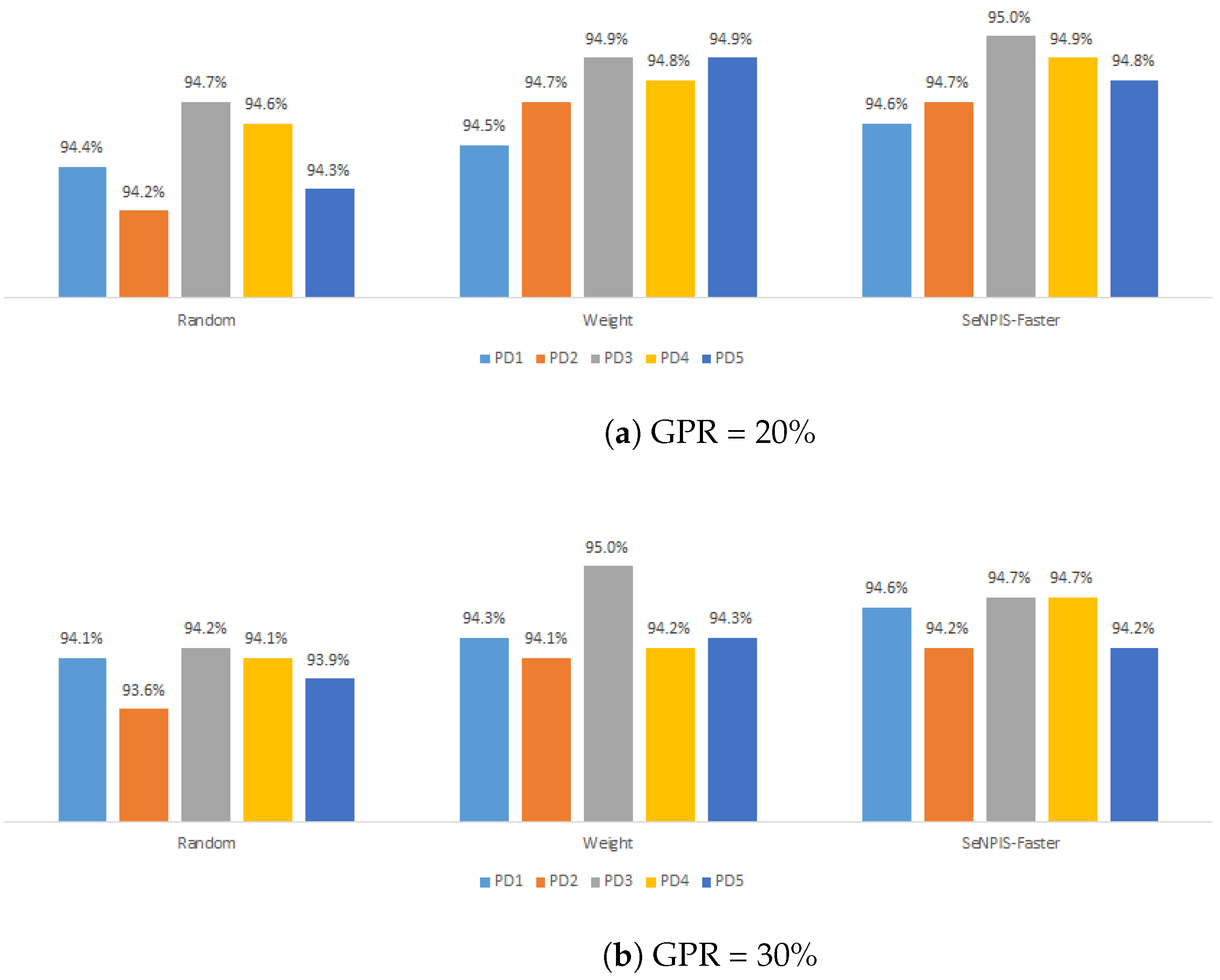
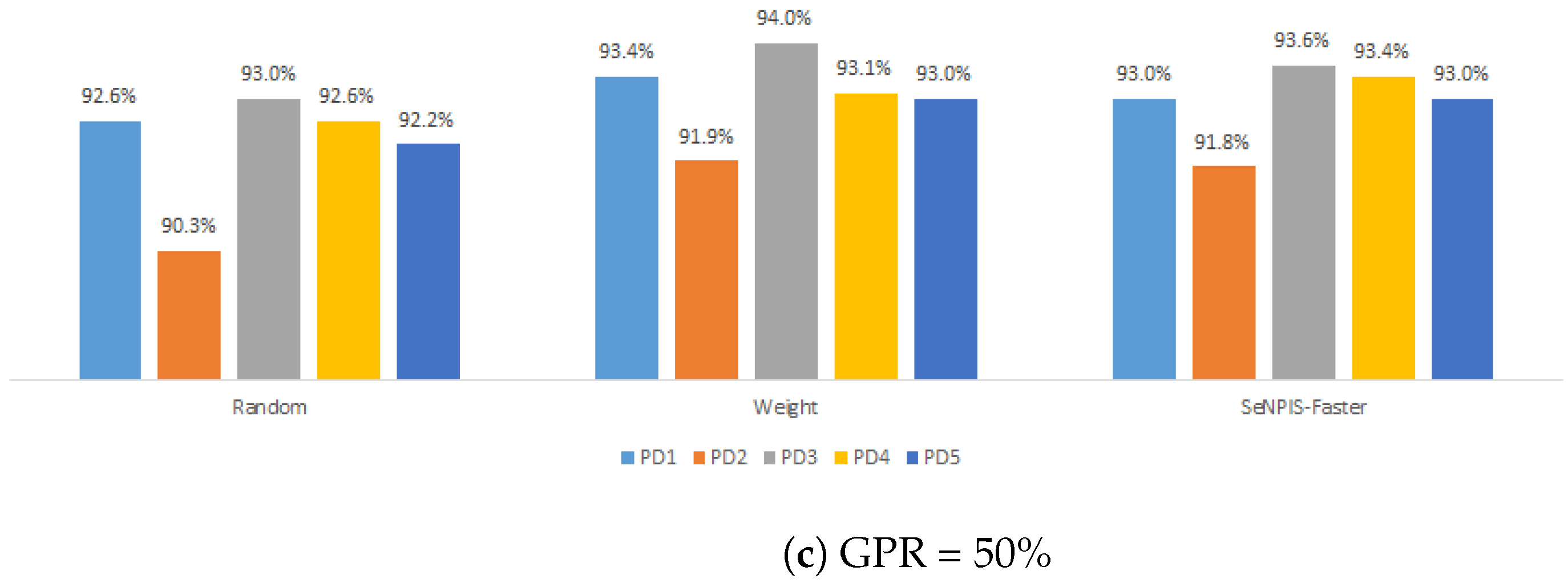
Figure 10 shows the results of the 45 pruned models—each bar represents one model. On the y-axis is the performance metric (accuracy was chosen for this case study because it is a balanced dataset), and on the x-axis is each of the methods with the five distribution types selected.

When GPR = 20% (Figure 10a), the best pair is SeNPIS-Faster with $P{D}_3$ (i.e., 95%), and the worst is Random with $P{D}_2$ (i.e., 94.2%). The difference between them is 0.8%.

When GPR = 30% (Figure 10b), the best pair is Weight with $P{D}_3$ (i.e., 95%), and the worst is Random with $P{D}_2$ (93.6%). The difference between them is 1.4%.

When GPR = 50% (Figure 10c), the best pair is Weight with $P{D}_3$ (i.e., 94%), and the worst is again Random with $P{D}_2$ (90.3%). The difference between them is 3.7%.

4.2.2. Impact of the Pruning Distribution

Figure 11 shows the corresponding results, where each bar represents the maximum difference in terms of the accuracy of five pruned models, the GPR and pruning method were fixed, and the PD was varied.

When GPR = 20%, the highest impact of PD is for Random (0.5%); when GPR = 30%, the highest impact is for Weight (0.9%). Finally, when GPR = 50%, the highest impact is for Random (2.7%).

4.2.3. Impact of the Pruning Method

Figure 12 shows the results, where each bar corresponds to the maximum difference in terms of the accuracy of three pruned models, the GPR and PD are fixed, and the pruning method was varied.

When GPR = 20%, the highest impact of the pruning method is for $P{D}_5$ (0.6%); when GPR = 30%, the highest impact is for $P{D}_3$ (0.8%). Finally, when GPR = 50%, the highest impact is for $P{D}_2$ (1.6%).

5. Discussion

This discussion section is divided into three parts. The first is related to the results obtained with the agriculture dataset. The second is related to the CIFAR10 dataset. And in the third, we will discuss the advantages of pruning in CNNs.

5.1. Case Study 1: Date Fruit Dataset

We will first focus on the agriculture dataset to discuss the results obtained. We will start with the question of what is more important, choosing the pruning method or the type of pruning distribution, to allows us to obtain a model performance that is as close as possible to that of the model without pruning.

In comparing the results in Figure 9 with those in Figure 10, it can be seen that when the GPR is 20%, there are greater differences in performance between the pruned models when the type of distribution is varied, up to 3.3%, compared to 2.7% when only the pruning method is varied. However, when the GPR value is increased to 30% and 50%, there is a greater impact on performance caused by the pruning method (4.7% and 10.6%, respectively) than that caused by the distribution type (3.4% and 6.7%, respectively). Thus, for this case study, we can summarize that the pruning method is slightly more important than the type of distribution when the GPR value is medium or high, while the type of pruning distribution is slightly more important for low GPR values.

On the other hand, is there a pruning policy (pruning method and distribution) that is significantly superior to the others, regardless of the GPR value? The answer is no; for example, Weight with $P{D}_1$, which works very well when the GPR is low and medium, performs poorly when the GPR is high. And SeNPIS-Faster with $P{D}_3$ works very well when the GPR is medium and high, but is the worst policy when the GPR is low. That is, a pruning policy that works very well for that classification problem (dataset) and a specific GPR value will not necessarily work well for a higher or lower GPR value.

In summary, from the analysis of the results obtained in this first case study, it is not possible to conclude that one pruning policy is significantly better or worse than another, nor can we affirm that the pruning method alone or the type of distribution alone is the most important thing. Therefore, when we have a highly complex dataset, such as that of the agricultural sector, it is necessary to apply a methodology that allows us to select the best pruning policy, and not just use the one recommended in another article or research, because it will not necessarily be the best option. And in considering that between the worst pruning policy and the best pruning policy the performance results can vary up to 12%, it becomes essential to select the right pruning policy.

5.2. Case Study 2: CIFAR10

Many CNN pruning studies perform their experimental phase with reference datasets such as CIFAR10 [46,47,48], and their proposed solutions are compared with other methods, but only using default pruning distribution. Therefore, it is not possible to identify whether the winning pruned model was better due to the type of method or due to the type of pruning distribution used. Authors often assume that it is due to the pruning method, but this is a mistake, and we will explain why below.

When the GPR is low or medium, the effect of the pruning distribution is very similar to that of the pruning method. It is less than 1% in all cases. This means that if a pruned model is the winner, the reason may be due to either of the pruning policy criteria, i.e., the method or distribution, since the level of impact is similar between them. However, when the GPR is high, say 50%, the pruning distribution has an even greater impact than the pruning method, so the winning pruning method may be due to the type of distribution used rather than the pruning method used.

In summary, when validating pruning studies with benchmark datasets such as CIFAR10, it is very difficult to assess the impact of the pruning method separately from that of the distribution type, unless a methodology such as that proposed in this article is used. This is the only way to objectively measure how much each pruning policy criterion has contributed to the performance of the pruned model.

5.3. Advantages of Pruning in CNNs

A recurring question when pruning CNNs is whether there is an advantage over the unpruned model. The goal of pruning is to obtain lighter models (bytes) and/or reduce FLOPs, with as little performance loss (in accuracy or F1) as possible. In the following, we will discuss the benefits of each.

In the case of parameters, reducing them allows the model to run on embedded systems or microcontrollers with low-memory specifications. Reducing parameters reduces the number of bytes in the model, so a pruned model that significantly reduces its parameters is useful for edge computing applications, for example.

In the case of FLOPs, this has a direct impact on the inference time ($IT$) of the pruned model, given that

$$IT={\displaystyle \frac{FLOPs}{FLOPS}},$$

(26)

where FLOPs are the floating-point operations, and they are obtained according to Equations (1)–(3); this means that it depends on the model. On the other hand, FLOPS are the floating-point operations per second; it depends on the hardware device. So, if we want to reduce the inference time of a model without improving the hardware device, we need to reduce the number of FLOPs in the model. The fewer FLOPs, the shorter the inference time (faster model).

The above shows a clear advantage of pruning, in that the bytes or FLOPs of the model can be reduced, but what about its performance? Typically, when the GPR value is increased, the accuracy or F1 of the pruned model decreases. However, there may be cases where a higher GPR value improves the performance of the model. For example, when using SeNPIS-Faster with $P{D}_2$ and $P{D}_3$ for the Date Fruit Dataset, or Weight with $P{D}_3$ for the CIFAR-10 dataset, the performance of the pruned models is better as the GPR increases from 20% to 30%. Even a pruned model may have a higher accuracy or F1 than the unpruned model (e.g., SeNPIS-Faster with $P{D}_5$ for the Data Fruit Dataset). This is because pruning the model removes filters that contributed little to the model’s decision making, or even hindered that decision making. In addition, after pruning, the weights can be fine-tuned to the classification problem at hand [49,50].

6. Conclusions

In the studies reporting the state-of-the-art methods, the importance of an adequate choice of the pruning policy, and not only of the pruning method, had not been demonstrated, since in most cases, the performance results of the pruned models had been reported using benchmark datasets of low complexity, such as CIFAR10, for which the impact of the pruning policy is not high (for example, around 3% between the best and worst pair of pruning methods vs. PD). Thanks to the proposed methodology and the study conducted, it could be observed that for more complex datasets, such as those of the agricultural sector, the performance of the pruned model varies significantly when the pruning policy is changed. For the same pruning method, but changing the PD, the differences can reach 7%, while for the same PD, but changing the pruning method, the differences can exceed 10%.

Therefore, it is recommended that future research on this topic should simultaneously include the pruning method and PD, especially when the application corresponds to medium- and high-complexity datasets, such as those in the agricultural sector.

Future research could test more benchmark datasets of different complexity. On the other hand, although the goal of this study was not to compare between pruning criteria but to show a methodology to select the best pruning policy regardless of the criterion, future research could conduct an exhaustive comparison of pruning criteria. Furthermore, the study could be extended to more types of CNN architectures than just VGG-16, such as RESNET or Inception-type architectures.

References

1. Simonyan, K.; Zisserman, A. Very deep convolutional networks for large-scale image recognition. arXiv 2014, arXiv:1409.1556. [Google Scholar]
2. He, K.; Zhang, X.; Ren, S.; Sun, J. Deep residual learning for image recognition. In Proceedings of the IEEE Conference on Computer Vision and Pattern Recognition, Las Vegas, NV, USA, 27–30 June 2016; pp. 770–778. [Google Scholar]
3. Altaheri, H.; Alsulaiman, M.; Muhammad, G. Date Fruit Classification for Robotic Harvesting in a Natural Environment Using Deep Learning. IEEE Access 2019, 7, 117115–117133. [Google Scholar] [CrossRef]
4. Du, J.; Zhang, M.; Teng, X.; Wang, Y.; Lim Law, C.; Fang, D.; Liu, K. Evaluation of vegetable sauerkraut quality during storage based on convolution neural network. Food Res. Int. 2023, 164, 112420. [Google Scholar] [CrossRef] [PubMed]
5. Li, S.; Zhang, S.; Xue, J.; Sun, H. Lightweight target detection for the field flat jujube based on improved YOLOv5. Comput. Electron. Agric. 2022, 202, 107391. [Google Scholar] [CrossRef]
6. Lin, J.; Chen, Y.; Pan, R.; Cao, T.; Cai, J.; Yu, D.; Chi, X.; Cernava, T.; Zhang, X.; Chen, X. CAMFFNet: A novel convolutional neural network model for tobacco disease image recognition. Comput. Electron. Agric. 2022, 202, 107390. [Google Scholar] [CrossRef]
7. Kamilaris, A.; Prenafeta-Boldú, F.X. Deep learning in agriculture: A survey. Comput. Electron. Agric. 2018, 147, 70–90. [Google Scholar] [CrossRef]
8. Luo, J.H.; Wu, J.; Lin, W. Thinet: A filter level pruning method for deep neural network compression. In Proceedings of the IEEE International Conference on Computer Vision, Venice, Italy, 22–29 October 2017; pp. 5058–5066. [Google Scholar]
9. Fountsop, A.N.; Ebongue Kedieng Fendji, J.L.; Atemkeng, M. Deep Learning Models Compression for Agricultural Plants. Appl. Sci. 2020, 10, 6866. [Google Scholar] [CrossRef]
10. Alqahtani, A.; Xie, X.; Jones, M.W. Literature Review of Deep Network Compression. Informatics 2021, 8, 77. [Google Scholar] [CrossRef]
11. Liang, T.; Glossner, J.; Wang, L.; Shi, S.; Zhang, X. Pruning and quantization for deep neural network acceleration: A survey. Neurocomputing 2021, 461, 370–403. [Google Scholar] [CrossRef]
12. Vadera, S.; Ameen, S. Methods for Pruning Deep Neural Networks. IEEE Access 2022, 10, 63280–63300. [Google Scholar] [CrossRef]
13. Reed, R. Pruning algorithms-a survey. IEEE Trans. Neural Netw. 1993, 4, 740–747. [Google Scholar] [CrossRef] [PubMed]
14. Sietsma, J.; Dow, R.J. Creating artificial neural networks that generalize. Neural Netw. 1991, 4, 67–79. [Google Scholar] [CrossRef]
15. Kavzoglu, T.; Mather, P.M. Pruning artificial neural networks: An example using land cover classification of multi-sensor images. Int. J. Remote Sens. 1999, 20, 2787–2803. [Google Scholar] [CrossRef]
16. Castellano, G.; Fanelli, A.; Pelillo, M. An iterative pruning algorithm for feedforward neural networks. IEEE Trans. Neural Netw. 1997, 8, 519–531. [Google Scholar] [CrossRef] [PubMed]
17. Arumuga Arun, R.; Umamaheswari, S. Effective multi-crop disease detection using pruned complete concatenated deep learning model. Expert Syst. Appl. 2023, 213, 118905. [Google Scholar] [CrossRef]
18. Ofori, M.; El-Gayar, O.; O’Brien, A.; Noteboom, C. A deep learning model compression and ensemble approach for weed detection. In Proceedings of the 55th Hawaii International Conference on System Sciences, Maui, HI, USA, 4–7 January 2022; pp. 1115–1124. [Google Scholar]
19. Fan, S.; Liang, X.; Huang, W.; Zhang, V.J.; Pang, Q.; He, X.; Li, L.; Zhang, C. Real-time defects detection for apple sorting using NIR cameras with pruning-based YOLOV4 network. Comput. Electron. Agric. 2022, 193, 106715. [Google Scholar] [CrossRef]
20. Shen, L.; Su, J.; He, R.; Song, L.; Huang, R.; Fang, Y.; Song, Y.; Su, B. Real-time tracking and counting of grape clusters in the field based on channel pruning with YOLOv5s. Comput. Electron. Agric. 2023, 206, 107662. [Google Scholar] [CrossRef]
21. Shi, R.; Li, T.; Yamaguchi, Y. An attribution-based pruning method for real-time mango detection with YOLO network. Comput. Electron. Agric. 2020, 169, 105214. [Google Scholar] [CrossRef]
22. Yvinec, E.; Dapogny, A.; Cord, M.; Bailly, K. Red: Looking for redundancies for data-freestructured compression of deep neural networks. Adv. Neural Inf. Process. Syst. 2021, 34, 20863–20873. [Google Scholar]
23. Liu, C.; Wu, H. Channel pruning based on mean gradient for accelerating convolutional neural networks. Signal Process. 2019, 156, 84–91. [Google Scholar] [CrossRef]
24. Guan, Y.; Liu, N.; Zhao, P.; Che, Z.; Bian, K.; Wang, Y.; Tang, J. Dais: Automatic channel pruning via differentiable annealing indicator search. IEEE Trans. Neural Netw. Learn. Syst. 2022, 34, 9847–9858. [Google Scholar] [CrossRef] [PubMed]
25. Wang, H.; Qin, C.; Zhang, Y.; Fu, Y. Neural pruning via growing regularization. arXiv 2020, arXiv:2012.09243. [Google Scholar]
26. Yeom, S.K.; Seegerer, P.; Lapuschkin, S.; Binder, A.; Wiedemann, S.; Müller, K.R.; Samek, W. Pruning by explaining: A novel criterion for deep neural network pruning. Pattern Recognit. 2021, 115, 107899. [Google Scholar] [CrossRef]
27. Meng, J.; Yang, L.; Shin, J.; Fan, D.; Seo, J.s. Contrastive Dual Gating: Learning Sparse Features With Contrastive Learning. In Proceedings of the IEEE/CVF Conference on Computer Vision and Pattern Recognition, New Orleans, LA, USA, 18–24 June 2022; pp. 12257–12265. [Google Scholar]
28. Pachón, C.G.; Ballesteros, D.M.; Renza, D. SeNPIS: Sequential Network Pruning by class-wise Importance Score. Appl. Soft Comput. 2022, 129, 109558. [Google Scholar] [CrossRef]
29. Han, S. Efficient Methods and Hardware for Deep Learning. Ph.D. Thesis, Stanford University, Stanford, CA, USA, 2017. [Google Scholar]
30. Li, H.; Kadav, A.; Durdanovic, I.; Samet, H.; Graf, H.P. Pruning filters for efficient convnets. arXiv 2016, arXiv:1608.08710. [Google Scholar]
31. Pachón, C.G.; Ballesteros, D.M.; Renza, D. An efficient deep learning model using network pruning for fake banknote recognition. Expert Syst. Appl. 2023, 233, 120961. [Google Scholar] [CrossRef]
32. Bragagnolo, A.; Barbano, C.A. Simplify: A Python library for optimizing pruned neural networks. SoftwareX 2022, 17, 100907. [Google Scholar] [CrossRef]
33. Mondal, M.; Das, B.; Roy, S.D.; Singh, P.; Lall, B.; Joshi, S.D. Adaptive CNN filter pruning using global importance metric. Comput. Vis. Image Underst. 2022, 222, 103511. [Google Scholar] [CrossRef]
34. Yang, C.; Liu, H. Channel pruning based on convolutional neural network sensitivity. Neurocomputing 2022, 507, 97–106. [Google Scholar] [CrossRef]
35. Chen, Z.; Liu, C.; Yang, W.; Li, K.; Li, K. LAP: Latency-aware automated pruning with dynamic-based filter selection. Neural Netw. 2022, 152, 407–418. [Google Scholar] [CrossRef]
36. Liu, Y.; Wu, D.; Zhou, W.; Fan, K.; Zhou, Z. EACP: An effective automatic channel pruning for neural networks. Neurocomputing 2023, 526, 131–142. [Google Scholar] [CrossRef]
37. Haar, L.V.; Elvira, T.; Ochoa, O. An analysis of explainability methods for convolutional neural networks. Eng. Appl. Artif. Intell. 2023, 117, 105606. [Google Scholar] [CrossRef]
38. LeCun, Y.; Bengio, Y.; Hinton, G. Deep learning. Nature 2015, 521, 436–444. [Google Scholar] [CrossRef] [PubMed]
39. Heaton, J. Ian Goodfellow, Yoshua Bengio, and Aaron Courville: Deep learning: The MIT Press, 2016, 800 pp, ISBN: 0262035618. Genet. Prog. Evolvable Mach. 2018, 19, 305–307. [Google Scholar] [CrossRef]
40. LeNail, A. Nn-svg: Publication-ready neural network architecture schematics. J. Open Source Softw. 2019, 4, 747. [Google Scholar] [CrossRef]
41. Cheng, Y.; Wang, D.; Zhou, P.; Zhang, T. Model compression and acceleration for deep neural networks: The principles, progress, and challenges. IEEE Signal Process Mag. 2018, 35, 126–136. [Google Scholar] [CrossRef]
42. Fu, L.; Yan, K.; Zhang, Y.; Chen, R.; Ma, Z.; Xu, F.; Zhu, T. EdgeCog: A Real-Time Bearing Fault Diagnosis System Based on Lightweight Edge Computing. IEEE Trans. Instrum. Meas 2023, 72, 1–11. [Google Scholar] [CrossRef]
43. Pachon, C.G.; Renza, D.; Ballesteros, D. Is My Pruned Model Trustworthy? PE-Score: A New CAM-Based Evaluation Metric. Big Data Cogn. Comput. 2023, 7, 111. [Google Scholar] [CrossRef]
44. Altaheri, H.; Alsulaiman, M.; Muhammad, G.; Amin, S.U.; Bencherif, M.; Mekhtiche, M. Date fruit dataset for intelligent harvesting. Data Brief 2019, 26, 104514. [Google Scholar] [CrossRef]
45. Krizhevsky, A.; Hinton, G. Learning Multiple Layers of Features from Tiny Images. 2009. Available online: https://www.cs.toronto.edu/~kriz/learning-features-2009-TR.pdf (accessed on 13 August 2024).
46. Jayasimhan, A.; Pabitha, P. ResPrune: An energy-efficient restorative filter pruning method using stochastic optimization for accelerating CNN. Pattern Recognit. 2024, 155, 110671. [Google Scholar] [CrossRef]
47. Yuan, T.; Li, Z.; Liu, B.; Tang, Y.; Liu, Y. ARPruning: An automatic channel pruning based on attention map ranking. Neural Netw. 2024, 174, 106220. [Google Scholar] [CrossRef] [PubMed]
48. Tmamna, J.; Ayed, E.B.; Fourati, R.; Hussain, A.; Ayed, M.B. A CNN pruning approach using constrained binary particle swarm optimization with a reduced search space for image classification. Appl. Soft Comput. 2024, 164, 111978. [Google Scholar] [CrossRef]
49. Baldi, P.; Sadowski, P.J. Understanding Dropout. In Proceedings of the Advances in Neural Information Processing Systems; Burges, C., Bottou, L., Welling, M., Ghahramani, Z., Weinberger, K., Eds.; Curran Associates, Inc.: Red Hook, NY, USA, 2013; Volume 26. [Google Scholar]
50. Wu, H.; Gu, X. Towards dropout training for convolutional neural networks. Neural Netw. 2015, 71, 1–10. [Google Scholar] [CrossRef] [PubMed]
Figure 1. Architecture of a convolutional neural network. It was generated using NN-SVG [40].
Informatics 11 00067 g001
Figure 2. Types of pruning distributions selected in this study. In uniform pruning ( P D 1 ), the same PR is pruned in all layers. In bottom-up pruning ( P D 2 ), the PR starts at a low value, but the deeper the network, the lower its value. In the case of top-down pruning ( P D 3 ), the PR starts at a high value, but the deeper the network, the lower its value. Bottom-up/top-down ( P D 4 ) starts and ends with a low PR, but in the intermediate layers, the value is higher than in the other layers. Finally, top-down/bottom-up ( P D 5 ) starts and ends with a high PR, but in the intermediate layers, the value is lower than in the other layers.
Informatics 11 00067 g002
Figure 3. Zeroing of pruned parameters or filter restructuring of the network; C is the number of channels, F is the filter layer, and H and W are the height and width of the input, respectively. The symbol (*) represents the convolution process between the input and the filter. With P R = 50%, F 1 , F 3 and F 5 are zeroed in the first case (represented by the black color), while they are deleted in the second case (and then only the F 2 , F 4 and F 6 filters appear).
Informatics 11 00067 g003
Figure 4. Overview of the proposed methodology for pruning policy selection. GPR is the global pruning rate, and PD is the pruning distribution.
Informatics 11 00067 g004
Figure 5. Samples of the Date Fruit Dataset for maturity classification. The first row shows date bunches where the dates are easily distinguished. The second row shows images where the bunches are far from the camera and with poor illumination, making it more difficult to recognize the maturity level of the dates.
Informatics 11 00067 g005
Figure 6. Pruning hyperparameters: GPR, PD, and pruning method.
Informatics 11 00067 g006
Figure 7. Date Fruit Dataset: F1 of pruned models for different GPRs (i.e., 20%, 30%, 50%), PDs (i.e., P D 1 to P D 5 ), and pruning methods (i.e., Random, Weight, and SeNPIS-Faster). The F1 of the unpruned model is 88.5%.
Informatics 11 00067 g007aInformatics 11 00067 g007b
Figure 8. Date Fruit Dataset: impact of the PD. Each bar corresponds to the difference between the best and worst PD, keeping the GPR and pruning method fixed.
Informatics 11 00067 g008
Figure 9. Date Fruit Dataset: impact of the pruning method. Each bar corresponds to the difference between the best and worst pruning method, keeping the GPR and distribution type fixed.
Informatics 11 00067 g009
Figure 10. CIFAR10: accuracy of the pruned models for different GPRs (i.e., 20%, 30%, 50%), PDs (i.e., P D 1 to P D 5 ), and pruning methods (i.e., Random, Weight, and SeNPIS-Faster). The a c c u r a c y of the unpruned model is 95.3%.
Informatics 11 00067 g010aInformatics 11 00067 g010b
Figure 11. CIFAR10: impact of the PD. Each bar corresponds to the difference in terms of the accuracy between the best and worst PD, keeping the GPR and pruning method fixed.
Informatics 11 00067 g011
Figure 12. CIFAR10: impact of the pruning method. Each bar corresponds to the difference in terms of accuracy between the best and worst pruning method, keeping the GPR and distribution type fixed.
Informatics 11 00067 g012