Abstract
CNN models can have millions of parameters, which makes them unattractive for some applications that require fast inference times or small memory footprints. To overcome this problem, one alternative is to identify and remove weights that have a small impact on the loss function of the algorithm, which is known as pruning. Typically, pruning methods are compared in terms of performance (e.g., accuracy), model size and inference speed. However, it is unusual to evaluate whether a pruned model preserves regions of importance in an image when performing inference. Consequently, we propose a metric to assess the impact of a pruning method based on images obtained by model interpretation (specifically, class activation maps). These images are spatially and spectrally compared and integrated by the harmonic mean for all samples in the test dataset. The results show that although the accuracy in a pruned model may remain relatively constant, the areas of attention for decision making are not necessarily preserved. Furthermore, the performance of pruning methods can be easily compared as a function of the proposed metric.
1. Introduction
Convolutional neural networks (CNNs) are deep learning models that provide competitive results on a variety of tasks such as image classification, object detection and semantic segmentation. However, advances in state-of-the-art deep learning methods usually involve an increase in complexity, number of parameters, amount of training resources or network latency. Accordingly, CNN models typically have tens (or even hundreds) of millions of parameters, making them unattractive for some applications that require fast inference times or small memory footprints. Hence, compression techniques have emerged to achieve more efficient representation (e.g., in terms of model size or inference latency) of one or more layers of a neural network in exchange for the least possible loss of quality. CNN model compression solutions include pruning, which helps reduce the size of the classification model—often with very little impact on performance. This can make CNNs more efficient and easier to deploy on mobile devices and other resource-constrained platforms.
Pruning techniques identify and remove weights that have a small impact on the loss function of the algorithm—i.e., weights that are not essential to the accuracy of the model—thereby reducing the model’s inference time (i.e., FLOPs) and its size (i.e., parameters) [1,2]. Pruning can be performed manually by a human expert or automatically by a computer algorithm; with structured pruning by removing layers, filters or channels [3] or with unstructured pruning by removing specific weights from the model regardless of their location in the network [4]. Structured pruning is usually preferred over unstructured pruning because the latter is difficult to use, as the hardware may not be able to efficiently run the network if the sparsity pattern is irregular.
Various pruning methods have been proposed in the literature, but the most common approach is based on the magnitude [5]. In this case, the feature maps (or filters) are sorted by their magnitudes, and the smallest ones are removed. This is because values with small magnitudes usually have a small impact on the model’s loss function [6]. Other methods use first- and second-order Taylor expansions of the loss function around a given neuron [7] or select the filters to be removed according to their class importance by evaluating the error function, as in the SeNPIS pruning method [8]. Recent methods proposed for pruning networks involve techniques to identify subnetworks that make training particularly effective with respect to the original network in a similar number of epochs [5]. Pruning methods that do not require any knowledge of the training data, i.e., data-agnostic pruning algorithms, have also been proposed. They are much faster and easier to use than other pruning algorithms that require training data [9].
Beyond the pruning method, approaches generally agree on how to evaluate the impact of pruning on the CNN architecture. First, a performance metric such as accuracy is used. That is, the performance of the original model is compared against the performance of the pruned model when using the same test dataset [10]. Second, the size of the model is evaluated in terms of the number of parameters or bytes, which is significant for the feasibility of implementing the model on resource-constrained platforms [11]. Finally, the time it takes to execute a CNN from a given input (inference speed) is also considered. This parameter can be measured in milliseconds, frames per second or other time units [12].
In any case, the selection of a pruning method is not a straightforward task, as it has implications on three fronts: loss of accuracy, selection of the pruning method and the pruning process used by the model. The loss of model accuracy takes on relevance when too many weights are removed, since the model may no longer be able to learn the same patterns in the data [10]. The selection of the pruning method for a particular application becomes complicated because there are many different pruning methods, and each has its own advantages and disadvantages in terms of size, performance or speed [11]. Regarding the pruning process, it is important to consider the time requirements and computational cost of the process, since it may be necessary to retrain the model after removing weights [10].
To overcome the challenge of assessing the impact of pruning, one alternative is to use model interpretation images (obtained by applying CAM-like techniques) to analyze whether the pruned model behaves similarly to the unpruned model; i.e., evaluate if the compressed model uses the same type of patterns to classify the image. In this case, the idea is to look at the activation map of the model after pruning and compare it with the activation map of the unpruned model to see if they are very similar. [10].
Under the above context, this paper proposes a metric to evaluate the impact of pruning on the CNN based on images obtained by applying CAM-based techniques to the pruned and unpruned models. This solution involves comparing the degree of similarity of the spatial structures of these maps as well as their levels of intensity through a spectral comparison of the maps. The spectral and spatial comparison is integrated through a harmonic mean, and it is calculated for all the examples in the test dataset. The idea is to determine whether the pruned model preserves the regions of importance of an image when making the inference.
The remainder of the paper is organized as follows. Section 2 presents basics of CNNs, model interpretation using CAM-type techniques, and pruning methods and their evaluation. Section 3 describes the materials and methods to obtain the proposed metric, which is named Sp2PS, for two models pre-trained on two datasets (CIFAR10 and STL10). Section 5 is focused on the conclusions of the study.
2. Background
2.1. Convolutional Neural Networks
A CNN is a type of artificial neural network commonly used for image recognition and processing. CNNs are based on the application of spatial filters using a cross-correlation operation to detect features in the input data, making them suitable for tasks such as image classification, image segmentation or object detection. CNNs are mainly built of three types of layers: convolutional, pooling and fully connected (FC). The first, convolutional layers, extract features from the input data by applying a set of convolutional filters or kernels that act on a small neighborhood (given by the size of the kernel) that is shifted along the entire input image. The parameters learned by the model correspond to the weights of these filters. The second corresponds to pooling layers, which are used to combine the information of contiguous spatial regions by means of an average pooling or maximum pooling operation; i.e., this type of layer reduces the size of the feature maps by taking the maximum value (max pooling) or the average value (average pooling) of each region. This helps to reduce the number of network parameters and make the network more efficient without adding additional parameters to the model. Finally, the third layer type, the FC layers, is oriented to perform the classification of the input image, so it is common to find it at the end of the network. In this case, the learned parameters correspond to the strength (weights) of the connection between neurons and their biases.
In addition, CNNs can have other types of layers: dropout and batch normalization (BN). They correspond to regularization techniques that try to prevent models from overfitting the training data in order to improve their generalization. Dropout randomly sets a certain percentage of input units to zero at each iteration during training (i.e., once the model is trained, no dropout is applied). This forces the network to learn to rely on other neurons to perform its tasks, which helps prevent it from becoming too dependent on a single set of neurons. On the other hand, BN calculates the mean and standard deviation of a layer’s activations to normalize them. BN helps to stabilize training by preventing activation values from becoming too large or too small. It also helps improve the generalization of the network by making it less sensitive to the distribution of the training data.
2.2. Model Interpretation Using CAM-Type Techniques
CAM-type techniques are used to interpret CNN models by identifying the regions of an input image that are most important for a given classification task [13]. Examples of class activation mapping methods are CAM, Grad-CAM, Grad-CAM++ and Ablation-CAM. CAM is the simplest of these methods since it calculates the importance of each input pixel through the activation maps of the last convolutional layer and then creates the heatmap by averaging the activation maps of all channels [14]. Grad-CAM (Gradient-Weighted CAM) is an evolution of CAM that calculates the importance of each pixel by means of the gradients of the final convolutional layer of the model with respect to the predicted class [14]. Grad-CAM++ is based on Grad-CAM but uses second-order gradients, so it obtains better results in terms of multiple appearances of a class in an image or in object localization [15]. Ablation CAM, on the other hand, is a CAM-like technique that does not rely on gradients. Instead, the importance of each pixel is calculated as a function of the reduction of the class activation score when its feature map is removed. Its output is obtained as the linear combination of the activation maps weighted by the corresponding importance values [16].
Figure 1 shows an example of CNN interpretation of an image of the STL10 dataset for Grad-CAM, Grad-CAM++ and Ablation-CAM methods. The more important pixels for the classification are the “red” ones, while the less important ones are the “blue” ones. Therefore, for the same model and with the same input image, there are small differences in the heat zones obtained by the three visualization methods. However, in all three cases, the most important pattern for classification corresponds to the deer antlers.
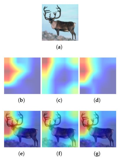
Figure 1.
Example of visualization using CAM-type techniques. Red: regions of major importance, blue: regions of minor importance in the class activation map. Dataset: STL10; methods: Grad-CAM, Grad-CAM++ and Ablation-CAM; class: deer (4th class). (a) Test image; (b) GradCAM; (c) GradCAM++; (d) Ablation CAM; (e) Overlay GradCAM; (f) Overlay GradCAM++; and (g) Overlay Ablation CAM.
2.3. Pruning Methods and Pruning Evaluation
As discussed so far, the application of pruning can be oriented to different purposes, such as reducing memory requirements, reducing the computational cost of inference, reducing power requirements, or improving network generalization [17]. For a neural network characterized by a set of parameters, pruning is a technique that allows obtaining a minimum subset of parameters by pruning or zeroing the remaining parameters. In turn, pruning ensures that model performance is preserved (above a given threshold) [18].
In the literature, pruning methods have been classified according to different aspects that may vary when implementing the pruning model. Consequently, recent classifications of pruning methods are structured according to the following aspects: estimation criterion, structure, distribution and scheduling [17,18,19].
The estimation criterion, also referred to as a scoring method or saliency metric, can be viewed similarly to a distance metric, such that it is used to measure and compare the importance of parameters for pruning. This category includes simple magnitude-based pruning methods [6,20], moment-based methods [21] or methods using metrics that approximate network sensitivity [22,23]. Methods initially developed to determine image saliency have also been applied as saliency metrics. For example, the contribution of the input dimension to the model decision has also been applied to pruning methods: in particular, Layered Relevance Propagation (LRP). In this case, the most relevant parameters are automatically determined using their relevance scores obtained from LRP [24]. A recently proposed method selects useful deep features from a discriminative dimension reduction perspective, through Fisher Linear Discriminant Analysis so that the method captures both the final separation of classes and their holistic inter-layer dependence [25]. The use of Amortized Explanation Models (AEMs) that utilize information from both inputs and outputs have also been proposed in order to predict in real-time smooth saliency masks and leverage the interpretations of the model to steer the pruning process [26]. It has also been proposed to evaluate gradient-based salience to measure the importance of a channel and to prune the lowest-scoring channels and their corresponding filters according to the pruning rate [27].
It is important to note that saliency measures have been used to: (i) estimate the effect of parameter removal on network performance, i.e., to propose new pruning methods and (ii) explain the results of image classifiers or interpret the classifier output [18]. Specifically, in the present paper, we do not propose a new pruning method, but we propose to use the interpretation of the classifier output to evaluate the performance of the pruned model with respect to the original model.
In the second aspect, structure, there are methods that can prune an entire block at a time: for example, a channel of a filter or a row of a weight matrix (structured pruning). As a counterpart, unstructured pruning treats all parameters equally [11,28,29]. Unstructured pruning is more flexible [5,30,31], whereas structured pruning may have advantages in terms of inference or storage times since whole blocks are omitted [18].
Regarding the classification by distribution, this refers to how the number of elements to be removed is distributed throughout the network [17]. In this case, it is possible to group all the parameters of the network and decide which parameters to prune (Global Distribution); i.e., prune the weights independently of the layer in which they appear. Included in this global distribution, for example, are methods that prune channels according to a threshold [32] or methods that prune channels that do not exceed a maximum degree of degradation in the final layer [33]. On the other hand, it is also possible to select how much to prune in each layer (layer-wise distribution), i.e., to consider that the pruning elements of different layers are part of different pruning pools [17,18]. There are also methods that determine the pruning rate of each layer based on sensitivity analysis [34,35] or reinforcement learning [36,37].
In addition to determining how to distribute the elements to be pruned, methods in the literature also consider when to perform the pruning [18]. It is possible to determine whether pruning is performed after, during or before training the network, so you have iterative methods or one-shot methods [17]. In the case of iterative methods, it is possible to have methods that prune an equal number of parameters in each round [6] or also methods that start by pruning at a high rate and then reduce the pruning rate [21].
Finally, it is important to consider that weight removal is usually accompanied by a strategy to repair the network, with fine tuning being the most common repair strategy [17].
Evaluation Metrics
Beyond the primary objective of a pruning method, pruning imposes a trade-off between efficiency (which generally increases) and performance of the pruned model (which generally decreases). Efficiency relates to the number of operations required to perform inference with the pruned model, which is usually represented by FLOPs. Model performance has a direct relationship to the fraction of pruned parameters, and it is usually evaluated by reporting changes in classification accuracy [19]. However, recent studies have shown the need for pruned network evaluation methods that go beyond accuracy and that can be used prior to model deployment. This is in order to provide new tools to help understand the over-parameterization of an architecture [38].
Also, although a pruned network may perform similarly to the original model in general tasks, it is important to keep in mind that the pruning potential of the network may vary significantly for a large number of tasks. This is particularly important in transfer-learning-based processes and also highlights the importance of performing complementary assessments of accuracy [19,38].
In this case, it is necessary to evaluate how pruning affects the function represented by a neural network, including the similarities and disparities exhibited by a pruned network with respect to its unpruned counterpart. Similarly, it is important to evaluate whether the use of a metric such as accuracy is sufficient to ensure that the pruned model performs well in the face of data generalization or phenomena such as noise [38].
Consequently, recent initiatives have considered establishing the maximum pruning ratio at which a model can retain similar functionality to the original model; this by means of metrics based on informative features and noise resilience [38]. The reliability of pruned models has also been assessed by comparing the explanation maps of the two models as well as class confidence [10].
In any case, it has been identified that new contributions are needed for the establishment of standardized parameters and metrics to assess whether the pruned models are functionally similar to the original models and their behavior on specific tasks [19,38].
3. Materials and Methods
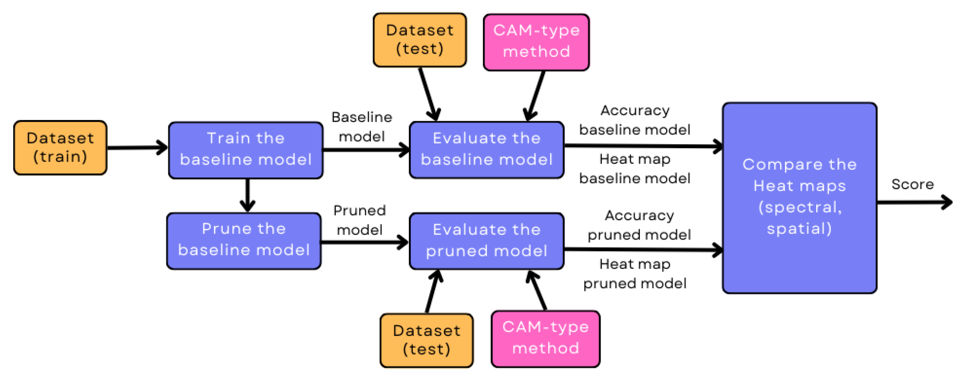
To evaluate whether the prediction of a pruned model is based on the same patterns as those of the unpruned model, this work proposes a methodology that includes the spatial and spectral similarity between heatmaps obtained with a CAM-type method. The idea is to have a procedure to evaluate and compare the performance of pruned models in a complementary way to the use of metrics that only rely on the confusion matrix but not on the patterns for model decision making.
The procedure to evaluate the similarity between the pruned and unpruned models is presented below:
- Select the dataset of the specific classification problem.
- Train a network with the selected dataset (or obtain a pre-trained model). The result is the baseline model.
- Prune the baseline model using a pruning method with a specific pruning rate and apply fine-tuning. The result is the pruned model.
- Evaluate the baseline model with the images belonging to the test dataset (or validation dataset) and obtain the accuracy of the baseline model. Subsequently, apply a CAM-type method to obtain the corresponding heatmaps of the baseline model.
- Evaluate the pruned model with the images belonging to the test dataset (or validation dataset) and obtain the accuracy of the pruned model. Subsequently, apply a CAM-type technique to obtain the corresponding heatmaps of the pruned model.
- Compare the spectral and spatial similarity for each pair of heatmaps from the baseline and pruned models.
Figure 2 shows the block diagram of the proposed methodology.
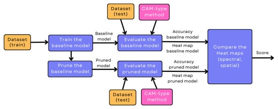
Figure 2.
Outline of the proposed methodology.
Each step of the methodology proposed in this study is described below.
3.1. Select the Dataset of the Specific Classification Problem
In this study, two of the most popular benchmark datasets for training and evaluating machine learning and computer vision models were selected: CIFAR10 [39] and STL10 [40]. In particular, they have been widely used to train and evaluate various ML models, including convolutional neural networks (CNNs). CIFAR10 consists of 60,000 natural-color images labeled and distributed in 10 classes with 6000 images per class. STL10 has 13,000 natural-color images labeled and distributed in 10 classes with 1300 images per class. Being natural images, they may contain noise and have high variability. Their difference lies in the spatial resolution: CIFAR10 images are of low resolution (), while STL10 images are of medium resolution in the context of deep learning (). The CIFAR10 classes are Airplane, Automobile, Bird, Cat, Deer, Dog, Frog, Horse, Ship and Truck; while in STL10, the same classes are preserved except for frog, which is replaced by monkey (organized in a different order).
3.2. Train a Network with the Selected Dataset or Obtain a Pre-Trained Model
This step consists of training a network with the selected dataset. For this particular study, we used two models that had previously been trained with the CIFAR10 and STL10 datasets and are available on GitHub under MIT license (https://github.com/aaron-xichen/pytorch-playground (accessed on 31 May 2023)). The accuracy of the first model is 93.78%, while in the second case, it is 77.59%.
The first network (see Figure 3a) consists of seven convolutional layers, four pooling layers and one fully connected (FC) layer. The second network (see Figure 3b) has six convolutional layers, five pooling layers and one FC layer.
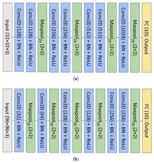
Figure 3.
Architecture of the baseline models obtained from GitHub (https://github.com/aaron-xichen/pytorch-playground (accessed on 31 May 2023)). For convolutional layers, kernel size: , stride and padding: . (a) Baseline model on CIFAR10; (b) Baseline model on STL10.
For calculation of the model parameters, the following equations are used:
where corresponds to the number of parameters in convolutional layers, is the width, is the height, and is the number of channels of the filters.
In the case of fully connected layers, the number of parameters, , is obtained as follows:
where is the number of neurons of the previous layer, and is the number of neurons in the current layer. On the other hand, pooling layers do not contribute parameters to the model.
In the case of FLOPs, the following equations are used:
where , and are the number of FLOPs in convolutional, fully connected and pooling layers, respectively; , and are the width, height and number of channels of the output of the layer; S is the stride of the kernel. For the convolutional and FC layers, the number of FLOPs is twice the input shape times the output shape of the layer.
For example, applying the above equations to the first network, the total number of parameters is about 9.3 million and the total number of FLOPs is about 1.3 G.
3.3. Prune the Baseline Model and Apply Fine Tuning
The pruning of the baseline models was applied globally to all tensors corresponding to the weights of the convolutional layers and to those of the FC. Pruning was performed in such a way that connections between units in adjacent layers were eliminated; i.e., the shape of the neural network was not changed. Thus, pruning was applied with one of the two global unstructured pruning methods available in PyTorch: Random and L1-norm. In the first case, the parameters to be pruned are determined randomly without any specific criteria; i.e., only the number or percentage of parameters to be pruned is defined. In the case of pruning based on the magnitude of the weights, the parameters with the lowest weight, determined by the L1-norm, are pruned. In either case, the amount of pruned parameters is a user-defined argument, and for the current study, it was varied from 20% to 80% in steps of 20%. Thus, by pruning part of the filters of the convolutional layers, the number of parameters and FLOPs of the model are reduced according to the equations presented previously. For example, in the first convolutional layer of the network shown in Figure 3a, there are 3584 parameters and 7,077,888 FLOPs before pruning. If 20% of the filters are eliminated, leaving 102 of the 128 filters, the number of parameters in this layer is 2856, and the number of FLOPs is 5,640,192.
In summary, the pruning methods used are as follows:
- Random pruning: global, structured and random pruning. Pruning applied to convolutional layer weights and FC layer weights. Pruning rates: [20% 40% 60% 80%].
- L1-norm pruning: global, structured and weight pruning (L1-norm). Pruning applied to convolutional layer weights and FC layer weights. Pruning rates: [20% 40% 60% 80%].
Once the models have been pruned, fine tuning is applied to repair the model. The general characteristics of the fine-tuning process are listed below:
- Dataset: training subset of the original distribution of the dataset;
- Batch size: 32;
- Optimizer and learning rate: stochastic gradient descent (SGD) with momentum (0.9), and learning rate: 0.001;
- Loss function: cross-entropy loss;
- Epochs: 10.
3.4. Evaluate the Baseline Model and the Pruned Model
From the two models (baseline and pruned), the accuracy of each is obtained using the test (or validation) images of the datasets selected in the study. These data correspond to 1000 test images per class in the case of CIFAR10 and 800 test images per class in the case of STL10. Heatmaps are then computed for each image using three CAM-type techniques, namely Grad-CAM, Grad-CAM++ and Ablation-CAM. The codes of these methods are available under MIT license at [41].
3.5. Compare the Heatmaps and Obtain the Score
From the images obtained in the previous step, each pair of heatmaps (obtained from the same test image, using the same CAM-type method for the baseline and the pruned models) is compared in terms of structural and spatial similarity. In this way, the degree of similarity between the pixels used by the pruned model for decision making and those of the baseline model is evaluated.
The comparison of spatial information of the images was performed through the structural similarity index (SSIM). The SSIM is a metric designed to evaluate the quality of one image relative to another taking into account aspects of luminance, contrast and structure. Its value can vary between 0 and 1, with 1 being the ideal or most similar case. For two images X and Y, the SSIM is given by Equation (6) [42].
where , , and correspond to the local means and variances of x and y, respectively, while is the covariance between x and y. On the other hand, and are two constants to stabilize the division.
On the other hand, the comparison of spectral information of the images was performed through the spectral angle mapper (SAM). This method allows determining the degree of spectral similarity of an image with respect to a reference spectrum (or with respect to another image) by calculating the angle between them. The pixel values of the two images are treated as a vector in a space whose dimension is equal to the number of bands. Roughly speaking, SAM calculates the similarity as the normalized dot product of the two vectors, as shown in Equation (7).
where represents the scalar product and denotes the norm.
Although Equation (7) gives a SAM value that can vary between 0 and , it can be normalized to values between zero ( radians, different spectra) and one (0 radians, similar spectra) so that its values also range between 0 and 1, as in the case of the SSIM. Under this context, 1 would be the ideal value: indicating absence of spectral distortion (but not necessarily equality of intensity).
Finally, the above metrics are combined into a single metric using the harmonic mean, which is similar to the F1-score in terms of precision and recall. The proposed evaluation metric, named Sp2PS, is presented by Equation (8):
where and correspond to the heatmap of the baseline and pruned model, and N is the total number of images in the test dataset. Since the SAM and SSIM values vary between 0 and 1, the proposed metric also varies between 0 and 1, where 1 indicates that the highlighted pixels of the pruned model are exactly the same as those of the baseline model.
4. Results and Discussion
In this section, we first present visual results that illustrate how the pruned models begin to divert attention to different areas of the image as the percentage of pruned parameters increases. Secondly, the consolidation of results for the entire dataset using the proposed metric is illustrated and compared to the accuracy results. All tests were performed using two pruning methods (i.e., L1-norm and Random) with four percentage rate (PR) values: i.e., 20%, 40%, 60% and 80%.
4.1. Preliminary Results
In order to observe how the decision areas of a model vary as the pruning percentage increases, the results for the three CAM-type techniques selected in this study are presented with some images from the CIFAR10 and STL10 datasets.
4.1.1. CIFAR10
Figure 4, Figure 5 and Figure 6 show the heatmaps using the CIFAR model and data and the Grad-CAM, Grad-CAM++ and Ablation-CAM methods, respectively. In all cases, the two selected pruning methods (i.e., L1-norm and Random) with the four selected percentage rates (PR), i.e., 20%, 40%, 60%, and 80%, are shown.

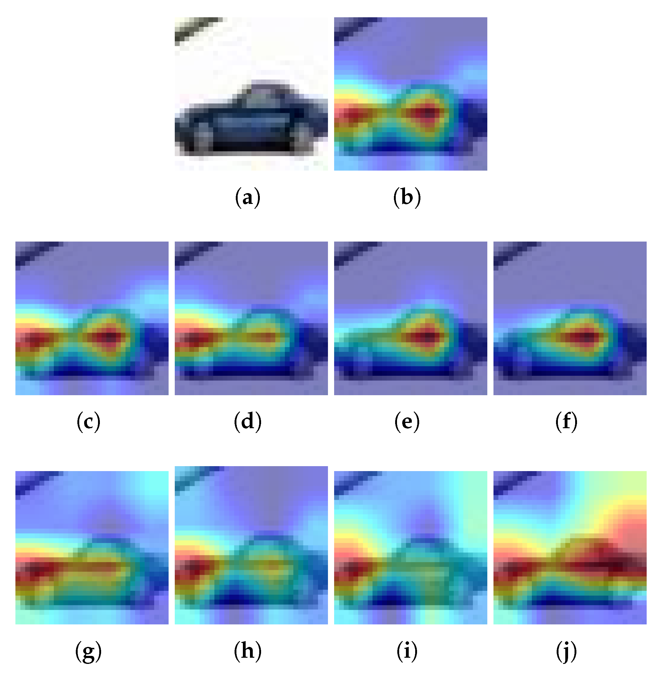
Figure 4.
Examples for CIFAR10 and Grad-CAM: (a) Input image, (b) Heatmap using the baseline model, (c–f) Heatmaps using a pruned model with L1-norm and PR = 20%, 40%, 60% and 80%, respectively, (g–j) Heatmap using a pruned model with Random and PR = 20%, 40%, 60% and 80%, respectively. is pruning rate.
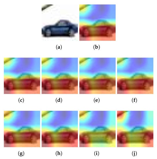
Figure 5.
Example for CIFAR10 and Grad-CAM++: (a) Input image, (b) Heatmap using the baseline model, (c–f) Heatmaps using a pruned model with L1-norm and PR = 20%, 40%, 60% and 80%, respectively, (g–j) Heatmaps using a pruned model with Random and PR = 20%, 40%, 60% and 80%, respectively. is pruning rate.
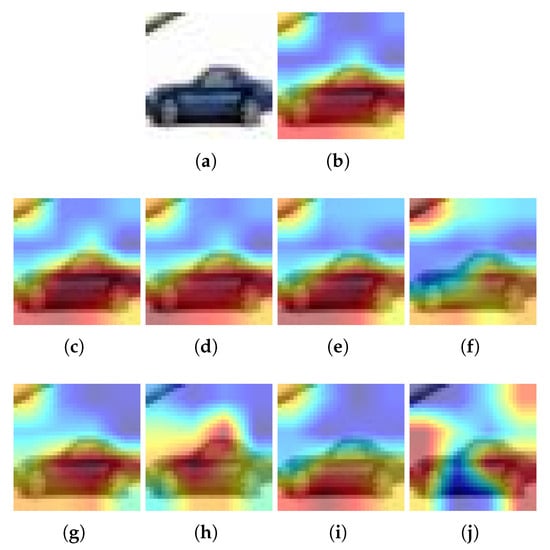
Figure 6.
Example for CIFAR10 and Ablation-CAM. (a) Input image, (b) Heatmap using the baseline model, (c–f) Heatmaps using a pruned model with L1-norm and PR = 20%, 40%, 60% and 80%, respectively; (g–j) Heatmaps using a pruned model with Random and PR = 20%, 40%, 60% and 80%, respectively. is pruning rate.
For Grad-CAM, when L1-norm is used as the pruning method, only the highlighted pixels of the image are retained when PR = 20%. In all other cases, the highlighted area becomes smaller (see Figure 4a). But when using the Random pruning method, the highlighted area changes significantly as the PR increases and takes other pixels that do not correspond to the class (see Figure 4b). On the other hand, using Grad-CAM++ and the L1-norm, it is obtained that the highlighted pixels of the image are preserved regardless of the PR value (see Figure 5a). However, when Random pruning is used, the area of interest decreases in size and is concentrated mainly on car tires when the PR is high (see Figure 5b). Finally, when using Ablation-CAM, we have that in the case of L1-norm, the highlighted pixels are preserved except when the PR is high: specifically, 80% (see Figure 6a); whereas when using Random pruning, there is a large difference in the highlighted pixels for PR values starting from 40% (see Figure 6b).
4.1.2. STL10
Figure 7, Figure 8 and Figure 9 show the heatmaps using the STL10 model and data and the Grad-CAM, Grad-CAM++ and Ablation-CAM methods, respectively. In all cases, the two selected pruning methods (i.e., L1-norm and Random) with the four selected PRs (i.e., 20%, 40%, 60% and 80%) are shown.
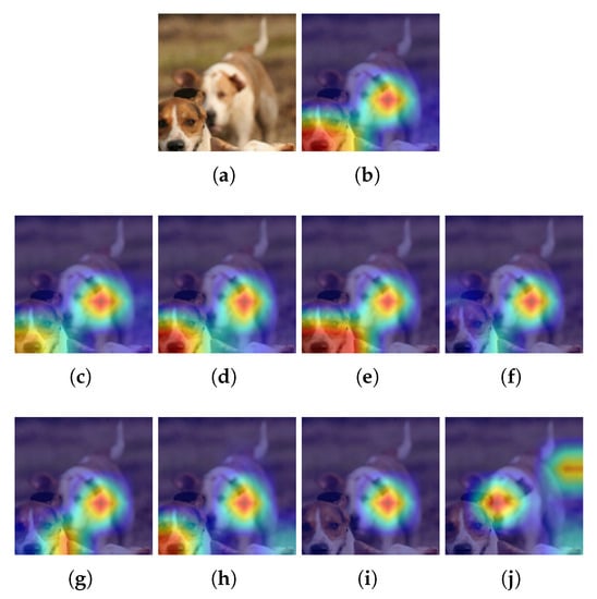
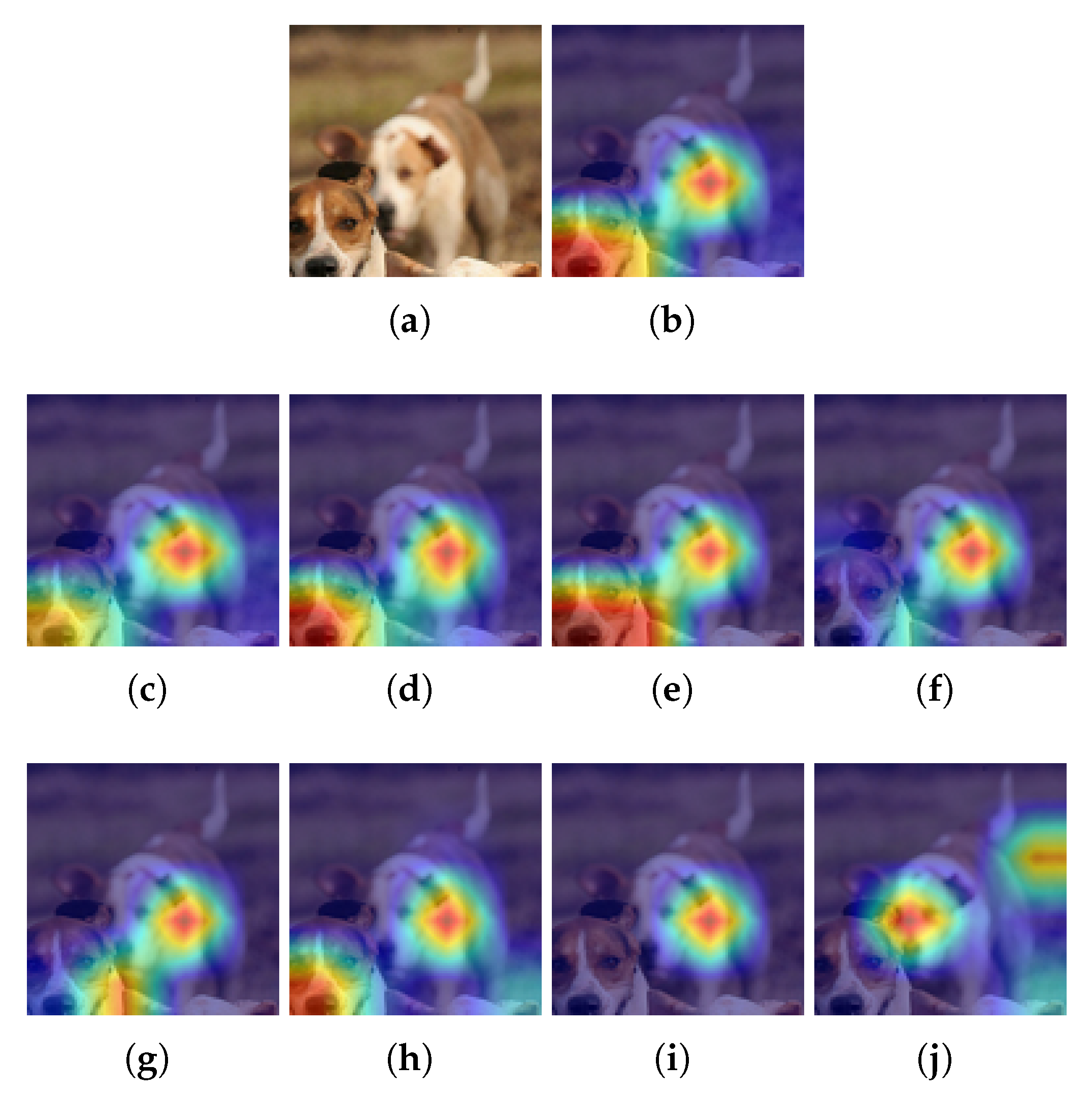
Figure 7.
Example for STL10 and Grad-CAM. (a) Input image, (b) Heatmap using the baseline model, (c–f) Heatmaps using a pruned model with L1-norm and PR = 20%, 40%, 60% and 80%, respectively; (g–j) Heatmaps using a pruned model with Random and PR = 20%, 40%, 60% and 80%, respectively. is pruning rate.
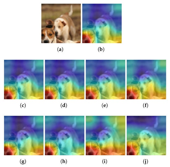
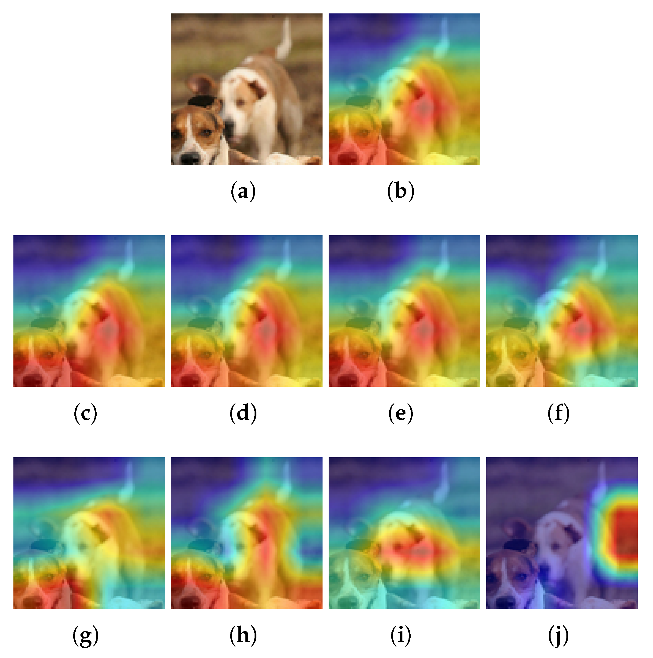
Figure 8.
Example for STL10 and Grad-CAM++. (a) Input image, (b) Heatmap using the baseline model, (c–f) Heatmaps using a pruned model with L1-norm and PR = 20%, 40%, 60% and 80%, respectively; (g–j) Heatmaps using a pruned model with Random and PR = 20%, 40%, 60% and 80%, respectively. is pruning rate.
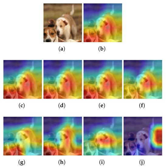
Figure 9.
Example for STL10 and Ablation-CAM. (a) Input image, (b) Heatmap using the baseline model, (c–f) Heatmaps using a pruned model with L1-norm and PR = 20%, 40%, 60% and 80%, respectively; (g–j) Heatmaps using a pruned model with Random and PR = 20%, 40%, 60% and 80%, respectively. is pruning rate.
With this dataset and using pruning with the L1-norm and Grad-CAM (see Figure 7a), it is found that for PR values of up to 60%, the pruned model focuses on almost the same pixels as in the baseline model; however, when there is a PR of 80%, it only focuses on the pixels of one of the dogs present in the image. Whereas in the case of Random pruning (see Figure 7b), the pruned model focuses on pixels similar to the baseline only for PR values up to 40%. When the PR is 80%, the pruned model focuses on pixels that do not correspond to the baseline.
On the other hand, when using Grad-CAM++ (see Figure 8) for the different PR values and with the two pruning methods, it is observed that the highlighted pixels of the pruned models are very similar to those of the baseline model.
Finally, when using Ablation-CAM, if the pruning method is L1-norm (see Figure 9a), it is observed that as the PR increases, the intensity of the highlighted pixels decreases in some areas of the image. In contrast, when pruning is Random (see Figure 9b), the area of interest changes significantly from a PR of 60%.
4.2. Consolidated Results
The consolidated results are presented below simultaneously in terms of the accuracy of the pruned model and the proposed metric, i.e., Sp2PS.
4.2.1. CIFAR10: Accuracy vs. Sp2PS
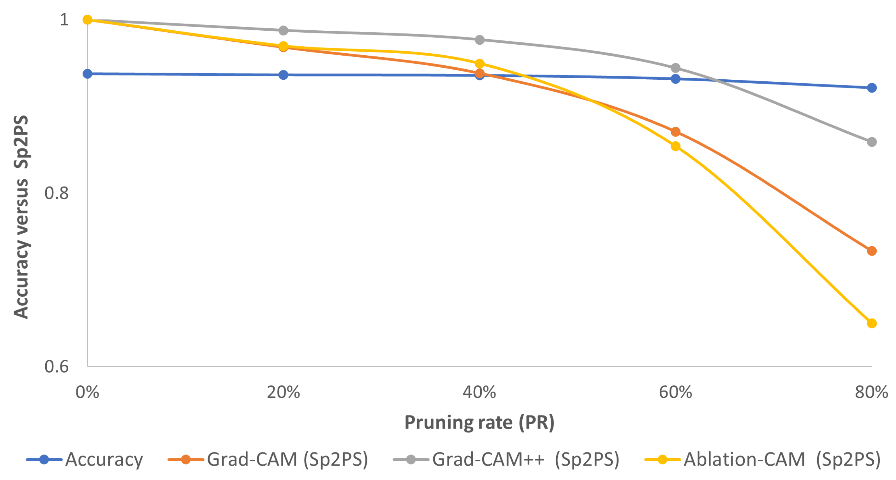
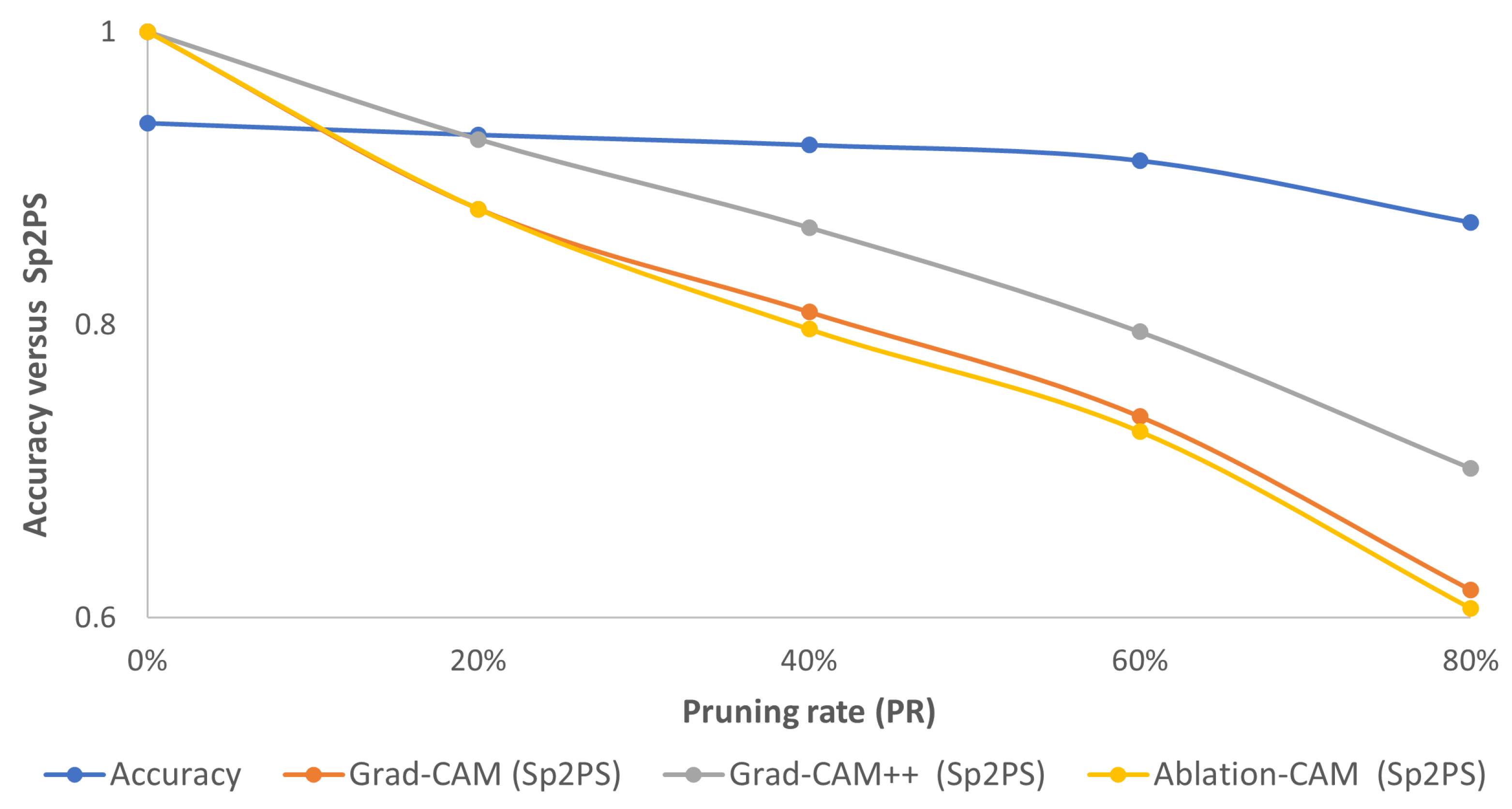
From Figure 4, Figure 5 and Figure 6, we can see that with L1-norm, the pruned model retains a good deal of attention on pixels similar to those of the unpruned model, mainly for PR values of 20% and 40%. Above 60%, the area of interest and/or the intensity of the highlighted pixels changes. Now, comparing the accuracy of the pruned model with the proposed metric (Figure 10), it is observed that for the three visualization methods—Grad-CAM, Grad-CAM++ and Ablation-CAM—the Sp2PS metric curves (orange, gray and yellow curves) remain relatively flat (as does the accuracy curve) for PRs up to 40%. For pruning percentages of 60% or more, the drop in Sp2PS is more noticeable; therefore, it is possible to identify the PR value at which the model stops focusing on similar zones (patterns) as those of the original model as the Sp2PS curve falls from its ideal value.

Figure 10.
Consolidated results for CIFAR10 using the L1-norm method: accuracy (blue curve) vs. Sp2PS. Grad-CAM (orange), Grad-CAM++ (gray) and Ablation-CAM (yellow). PR = 20%, 40%, 60% and 80%.
For the case of Random pruning, from Figure 4, Figure 5 and Figure 6, it is observed that only when the PR is equal to 20% is there moderately acceptable similarity between the behavior of the pruned model and the baseline model. In this case, by comparing the trend of accuracy with respect to the proposed metric (Figure 11), it is observed that even when the PR is equal to 20%, the slope of the fall of the Sp2PS metric is more noticeable than in the case of the models pruned with the L1-norm; so a flat trend is not maintained as in the accuracy curve.
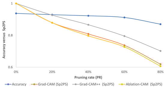
Figure 11.
Consolidated results for CIFAR10 using the Random method: accuracy (blue curve) vs. Sp2PS. Grad-CAM (orange), Grad-CAM++ (gray) and Ablation-CAM (yellow). PR = 20%, 40%, 60% and 80%.
4.2.2. STL10: Accuracy vs. Sp2PS
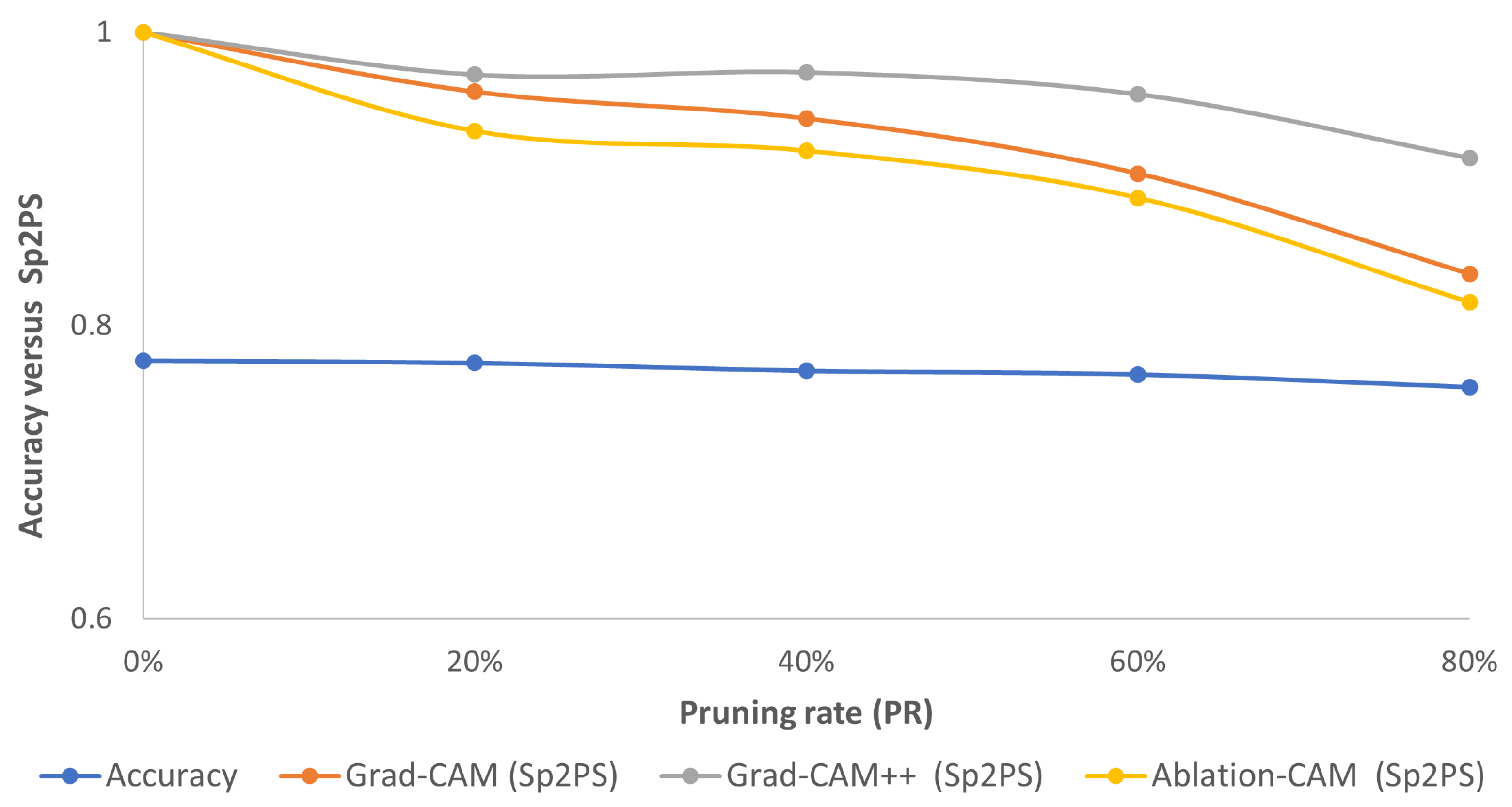
For this dataset, according to Figure 7, Figure 8 and Figure 9, the highlighted pixels of the pruned models using the L1-norm are very similar to those of the reference model for the three CAM-type visualization methods mainly for pruning values up to 60%. Now, if we observe accuracy and Sp2PS values (see Figure 12), we see that for the three CAM-type techniques, the Sp2PS curves present a relatively constant and high value for the first three PR values, which means that these pruned models obtained with the L1-norm method are centered on the same (or almost the same) pixels as in the reference model. When PR = 80%, a greater reduction in Sp2PS is presented, which implies the image areas used by the model for decision making differ to a greater extent.
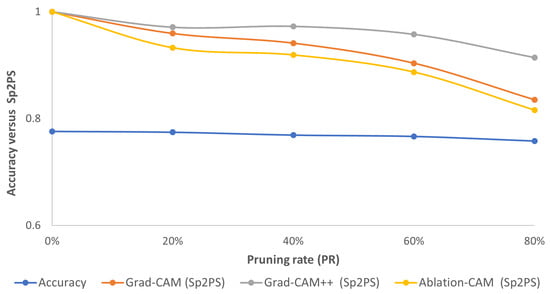
Figure 12.
Consolidated results for STL10 using the L1-norm method: accuracy (blue curve) vs. Sp2PS. Grad-CAM (orange), Grad-CAM++ (gray) and Ablation-CAM (yellow). PR = 20%, 40%, 60% and 80%.
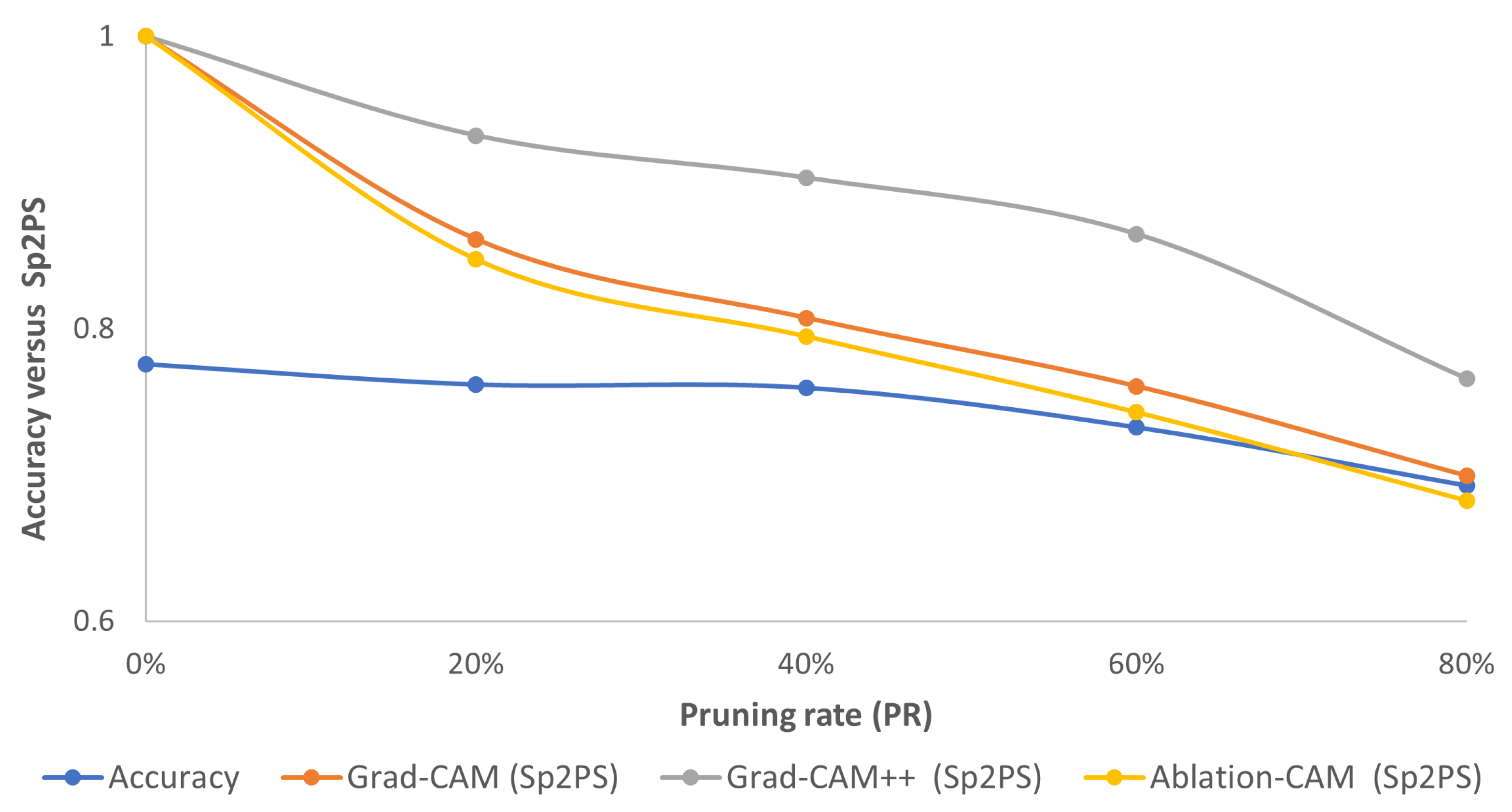
Finally, when random pruning is performed, it is observed that with low PR values the pruned model focuses on almost the same pixels as the base model, but it can vary its intensity (color); while with high PR values, it focuses on other pixels not related to the object to be classified. When plotting the accuracy versus Sp2PS curves with the three CAM-type techniques (see Figure 13), it is observed that from PR = 20%, the three Sp2PS curves move away from their ideal values. Thus, in general terms, although these randomly pruned models may retain a close value of accuracy, they focus on different types of patterns than those identified by the baseline model.
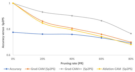
Figure 13.
Consolidated results for STL10 using the Random method: accuracy (blue curve) vs. Sp2PS. Grad-CAM (orange), Grad-CAM++ (gray) and Ablation-CAM (yellow). PR = 20%, 40%, 60% and 80%.
In any case, it is important to note that in pruned models, although the accuracy may remain relatively constant, the zones of attention for decision making are not necessarily retained, according to the trend of the Sp2PS metric. Additionally, Figure 10, Figure 11, Figure 12 and Figure 13 allow us to compare the behavior of the pruning methods (L1-norm and Random) where, as expected, the pruning by magnitude tries to better preserve the behavior of the baseline model.
4.3. Comparison with the State-of-the-Art
To the best of our knowledge, the state-of-the-art of evaluation metrics for pruning methods based on CAM-type techniques only includes the PE-score (when referring to pruning impact evaluation and not the estimation criteria) [10]. The main difference between PE-scores and the one proposed in this paper (i.e., Sp2PS) is that the calculation of PE-scores uses two measurements between the feature maps of the baseline and the pruned model (specifically, SSIM and IoU) and a measurement of the confidence variation, whereas in our case, Sp2PS uses only two measurements between the feature maps of these models (specifically, SSIM and SAM).
The objective of this section is to compare the results obtained with both metrics using a sequential model for the CIFAR10 dataset and to determine if there are similarities or differences in their behavior. In both cases, the relationship between the drop in accuracy (i.e., the decrease in accuracy of the pruned model relative to the baseline model) and the decrease in the interpretability metric (specifically, and ) as the pruning rate (PR) is varied will be compared. This comparison is made by considering the CAM-type method used to calculate the interpretability metric.
First, the ablation method is used, the results of which are shown in Table 1. In both cases, the values of and increase as increases. This means that for higher values of PR (note that is the lowest, while is the highest), the accuracy of the model always decreases (i.e., increases), as does the value of the interpretability metric. However, for similar values of (from 1.5% approximately), there are higher values of than of , which means that the proposed interpretability metric is more sensitive to small changes in model accuracy than the PE-score. This condition can be very useful in image classification problems where the decrease in the pruned model should be as small as possible, e.g., less than 2%, as in the case of biomedical applications.

Table 1.
Comparison of vs. (; ) when the Ablation method is used. Model and dataset: CIFAR10.
As a second part of this comparison, Table 2 shows the results when GradCAM is used to calculate the interpretability metrics. Behavior similar to that obtained when using the Ablation method to calculate Sp2PS and PE is observed. For values above 1.6% accuracy drop, the metric has much higher values than the metric. For example, when = 1.60%, an of 35% is obtained, while a of 30% is reached at of 3.63%. Again, this can be useful in applications that require pruned models that are highly similar in terms of performance to unpruned models, i.e., an lower than 2%.
Table 2.
Comparison of vs. (; ) when the GradCAM method is used. Model and dataset: CIFAR10.
Finally, we have the results when using the GradCAM++ method (see Table 3). As in the previous two cases, the drop in the interpretability metric is more noticeable in the Sp2PS case than in the PE case.
Table 3.
Comparisons of vs. and vs. . CAM-type method: Ablation. Model and dataset: CIFAR10.
5. Conclusions
In this paper, we proposed a metric to evaluate whether a pruned model focuses on the same patterns as the unpruned model based on the analysis of the structural and spectral similarity between the heatmaps of the two models obtained with CAM-type visualization techniques. It was found that although the accuracy of the pruned model is close to that of the baseline model, the behavior of the pruned model may be significantly different from that of the baseline model. From the accuracy curves against the proposed metric, called Sp2PS, it is possible to identify the PR value at which the pruned model ceases to be trustworthy (in the sense that it no longer focuses on the same patterns as the baseline model). According to the experiments carried out, the Sp2PS values are higher when using Grad-CAM++, and very similar values are obtained between Grad-CAM and Ablation-CAM. Thus, two thresholds are proposed to be able to trust the pruned model: 0.95 for Grad-CAM and 0.9 for Ablation-CAM. In addition, the proposed metric has been evaluated in relation to the drop in accuracy, proving that the proposed interpretability metric is sensitive to small changes in model accuracy. Finally, this metric is then proposed as a complementary metric to evaluate the quality of a pruned model.
Author Contributions
Conceptualization, D.R. and D.B.; Methodology, D.R.; Software, D.R.; Validation, D.R.; Formal analysis, D.B.; Investigation, D.R. and D.B.; Writing—original draft, D.R.; Writing—review and editing, D.B.; Funding acquisition, D.B. and D.R. All authors have read and agreed to the published version of the manuscript.
Funding
This work has been sponsored by the Universidad Militar Nueva Granada—Vicerrectoría de investigaciones, with project INV-ING-3786, entitled “Compression of deep learning models for image classification tasks applied to industry 4.0”.
Institutional Review Board Statement
Not applicable.
Data Availability Statement
Not applicable.
Conflicts of Interest
The authors declare no conflict of interest.
Abbreviations
The following abbreviations are used in this manuscript:
| CNN | Convolutional Neural Network |
| CAM | Class Activation Map |
| SAM | Spectral Angle Mapper |
| SSIM | Structural Similarity Index |
| PR | Pruning Rate |
References
- You, Z.; Yan, K.; Ye, J.; Ma, M.; Wang, P. Gate decorator: Global filter pruning method for accelerating deep convolutional neural networks. Adv. Neural Inf. Process. Syst. 2019, 32. Available online: https://proceedings.neurips.cc/paper_files/paper/2019/file/b51a15f382ac914391a58850ab343b00-Paper.pdf (accessed on 15 August 2023).
- Hou, Y.; Ma, Z.; Liu, C.; Wang, Z.; Loy, C.C. Network pruning via resource reallocation. Pattern Recognit. 2023. [Google Scholar] [CrossRef]
- Fang, G.; Ma, X.; Song, M.; Mi, M.B.; Wang, X. Depgraph: Towards any structural pruning. In Proceedings of the IEEE/CVF Conference on Computer Vision and Pattern Recognition, Vancouver, BC, Canada, 17–24 June 2023; pp. 16091–16101. [Google Scholar]
- Kwon, S.J.; Lee, D.; Kim, B.; Kapoor, P.; Park, B.; Wei, G.Y. Structured compression by weight encryption for unstructured pruning and quantization. In Proceedings of the IEEE/CVF Conference on Computer Vision and Pattern Recognition, Seattle, WA, USA, 13–19 June 2020; pp. 1909–1918. [Google Scholar]
- Frankle, J.; Carbin, M. The lottery ticket hypothesis: Finding sparse, trainable neural networks. arXiv 2018, arXiv:1803.03635. [Google Scholar]
- Han, S.; Pool, J.; Tran, J.; Dally, W. Learning both weights and connections for efficient neural network. Adv. Neural Inf. Process. Syst. 2015, 28, 1135–1143. [Google Scholar]
- Molchanov, P.; Mallya, A.; Tyree, S.; Frosio, I.; Kautz, J. Importance estimation for neural network pruning. In Proceedings of the IEEE/CVF Conference on Computer Vision and Pattern Recognition, Long Beach, CA, USA, 15–20 June 2019; pp. 11264–11272. [Google Scholar]
- Pachón, C.G.; Ballesteros, D.M.; Renza, D. SeNPIS: Sequential Network Pruning by class-wise Importance Score. Appl. Soft Comput. 2022, 129, 109558. [Google Scholar]
- Tanaka, H.; Kunin, D.; Yamins, D.L.; Ganguli, S. Pruning neural networks without any data by iteratively conserving synaptic flow. Adv. Neural Inf. Process. Syst. 2020, 33, 6377–6389. [Google Scholar]
- Pachon, C.G.; Renza, D.; Ballesteros, D. Is My Pruned Model Trustworthy? PE-Score: A New CAM-Based Evaluation Metric. Big Data Cogn. Comput. 2023, 7, 111. [Google Scholar]
- Molchanov, P.; Tyree, S.; Karras, T.; Aila, T.; Kautz, J. Pruning convolutional neural networks for resource efficient inference. arXiv 2016, arXiv:1611.06440. [Google Scholar]
- Luo, J.H.; Wu, J. Autopruner: An end-to-end trainable filter pruning method for efficient deep model inference. Pattern Recognit. 2020, 107, 107461. [Google Scholar]
- Jung, H.; Oh, Y. Towards better explanations of class activation mapping. In Proceedings of the IEEE/CVF International Conference on Computer Vision, Montreal, BC, Canada, 10–17 October 2021; pp. 1336–1344. [Google Scholar]
- Selvaraju, R.R.; Cogswell, M.; Das, A.; Vedantam, R.; Parikh, D.; Batra, D. Grad-cam: Visual explanations from deep networks via gradient-based localization. In Proceedings of the IEEE International Conference on Computer Vision, Venice, Italy, 22–29 October 2017; pp. 618–626. [Google Scholar]
- Chattopadhay, A.; Sarkar, A.; Howlader, P.; Balasubramanian, V.N. Grad-cam++: Generalized gradient-based visual explanations for deep convolutional networks. In Proceedings of the 2018 IEEE Winter Conference on Applications of Computer Vision (WACV), Lake Tahoe, NV, USA, 12–15 March 2018; pp. 839–847. [Google Scholar]
- Ramaswamy, H.G. Ablation-cam: Visual explanations for deep convolutional network via gradient-free localization. In Proceedings of the IEEE/CVF Winter Conference on Applications of Computer Vision, Snowmass, CO, USA, 1–5 March 2020; pp. 983–991. [Google Scholar]
- Persand, K.D. Improving Saliency Metrics for Channel Pruning of Convolutional Neural Networks. Ph.D. Thesis, Trinity College Dublin, Dublin, Ireland, 2022. [Google Scholar]
- Menghani, G. Efficient deep learning: A survey on making deep learning models smaller, faster, and better. ACM Comput. Surv. 2023, 55, 1–37. [Google Scholar]
- Blalock, D.; Gonzalez Ortiz, J.J.; Frankle, J.; Guttag, J. What is the state of neural network pruning? Proc. Mach. Learn. Syst. 2020, 2, 129–146. [Google Scholar]
- Mao, H.; Han, S.; Pool, J.; Li, W.; Liu, X.; Wang, Y.; Dally, W.J. Exploring the granularity of sparsity in convolutional neural networks. In Proceedings of the IEEE Conference on Computer Vision and Pattern Recognition Workshops, Honolulu, HI, USA, 21–26 July 2017; pp. 13–20. [Google Scholar]
- Dettmers, T.; Zettlemoyer, L. Sparse Networks from Scratch: Faster Training without Losing Performance. arXiv 2019, arXiv:cs.LG/1907.04840. [Google Scholar]
- Theis, L.; Korshunova, I.; Tejani, A.; Huszár, F. Faster gaze prediction with dense networks and fisher pruning. arXiv 2018, arXiv:1801.05787. [Google Scholar]
- Ding, X.; Zhou, X.; Guo, Y.; Han, J.; Liu, J. Global sparse momentum sgd for pruning very deep neural networks. Adv. Neural Inf. Process. Syst. 2019, 32, 6382–6394. [Google Scholar]
- Yeom, S.K.; Seegerer, P.; Lapuschkin, S.; Binder, A.; Wiedemann, S.; Müller, K.R.; Samek, W. Pruning by explaining: A novel criterion for deep neural network pruning. Pattern Recognit. 2021, 115, 107899. [Google Scholar] [CrossRef]
- Tian, Q.; Arbel, T.; Clark, J.J. Task dependent deep LDA pruning of neural networks. Comput. Vis. Image Underst. 2021, 203, 103154. [Google Scholar] [CrossRef]
- Ganjdanesh, A.; Gao, S.; Huang, H. Interpretations steered network pruning via amortized inferred saliency maps. In Proceedings of the European Conference on Computer Vision, Tel Aviv, Israel, 23–27 October 2022; Springer: Berlin/Heidelberg, Germany, 2022; pp. 278–296. [Google Scholar]
- Choi, J.I.; Tian, Q. Visual Saliency-Guided Channel Pruning for Deep Visual Detectors in Autonomous Driving. arXiv 2023, arXiv:2303.02512. [Google Scholar]
- Anwar, S.; Hwang, K.; Sung, W. Structured pruning of deep convolutional neural networks. ACM J. Emerg. Technol. Comput. Syst. (JETC) 2017, 13, 1–18. [Google Scholar] [CrossRef]
- Li, H.; Kadav, A.; Durdanovic, I.; Samet, H.; Graf, H.P. Pruning filters for efficient convnets. arXiv 2016, arXiv:1608.08710. [Google Scholar]
- Wang, Z.; Li, F.; Shi, G.; Xie, X.; Wang, F. Network pruning using sparse learning and genetic algorithm. Neurocomputing 2020, 404, 247–256. [Google Scholar] [CrossRef]
- Liu, X.; Pool, J.; Han, S.; Dally, W.J. Efficient sparse-winograd convolutional neural networks. arXiv 2018, arXiv:1802.06367. [Google Scholar]
- Lin, S.; Ji, R.; Li, Y.; Wu, Y.; Huang, F.; Zhang, B. Accelerating Convolutional Networks via Global & Dynamic Filter Pruning. In Proceedings of the 27th International Joint Conference on Artificial Intelligence, Stockholm, Sweden, 13–19 July 2018; Volume 2, p. 8. [Google Scholar]
- Yu, R.; Li, A.; Chen, C.F.; Lai, J.H.; Morariu, V.I.; Han, X.; Gao, M.; Lin, C.Y.; Davis, L.S. Nisp: Pruning networks using neuron importance score propagation. In Proceedings of the IEEE Conference on Computer Vision and Pattern Recognition, Salt Lake City, UT, USA, 18–23 June 2018; pp. 9194–9203. [Google Scholar]
- Sabih, M.; Mishra, A.; Hannig, F.; Teich, J. MOSP: Multi-objective sensitivity pruning of deep neural networks. In Proceedings of the 2022 IEEE 13th International Green and Sustainable Computing Conference (IGSC), Pittsburgh, PA, USA, 24–25 October 2022; pp. 1–8. [Google Scholar]
- Sabih, M.; Yayla, M.; Hannig, F.; Teich, J.; Chen, J.J. Robust and Tiny Binary Neural Networks using Gradient-based Explainability Methods. In Proceedings of the 3rd Workshop on Machine Learning and Systems, Rome, Italy, 8 May 2023; pp. 87–93. [Google Scholar]
- Hirsch, L.; Katz, G. Multi-objective pruning of dense neural networks using deep reinforcement learning. Inf. Sci. 2022, 610, 381–400. [Google Scholar] [CrossRef]
- Yang, W.; Yu, H.; Cui, B.; Sui, R.; Gu, T. Deep neural network pruning method based on sensitive layers and reinforcement learning. Artif. Intell. Rev. 2023, 1–21. [Google Scholar] [CrossRef]
- Liebenwein, L.; Baykal, C.; Carter, B.; Gifford, D.; Rus, D. Lost in pruning: The effects of pruning neural networks beyond test accuracy. Proc. Mach. Learn. Syst. 2021, 3, 93–138. [Google Scholar]
- Krizhevsky, A.; Hinton, G. Learning Multiple Layers of Features from Tiny Images. 2009. Available online: http://www.cs.utoronto.ca/~kriz/learning-features-2009-TR.pdf (accessed on 15 May 2023).
- Coates, A.; Ng, A.; Lee, H. An analysis of single-layer networks in unsupervised feature learning. In Proceedings of the Fourteenth International Conference on Artificial Intelligence and Statistics, JMLR Workshop and Conference Proceedings, Fort Lauderdale, FL, USA, 13–15 April 2011; pp. 215–223. [Google Scholar]
- Gildenblat, J. PyTorch Library for CAM Methods. 2021. Available online: https://github.com/jacobgil/pytorch-grad-cam (accessed on 1 May 2023).
- Wang, Z.; Bovik, A.C.; Sheikh, H.R.; Simoncelli, E.P. Image quality assessment: From error visibility to structural similarity. IEEE Trans. Image Process. 2004, 13, 600–612. [Google Scholar] [CrossRef] [PubMed]


Disclaimer/Publisher’s Note: The statements, opinions and data contained in all publications are solely those of the individual author(s) and contributor(s) and not of MDPI and/or the editor(s). MDPI and/or the editor(s) disclaim responsibility for any injury to people or property resulting from any ideas, methods, instructions or products referred to in the content. |
© 2023 by the authors. Licensee MDPI, Basel, Switzerland. This article is an open access article distributed under the terms and conditions of the Creative Commons Attribution (CC BY) license (https://creativecommons.org/licenses/by/4.0/).