Article

Towards Moving Objects Behavior Analysis: Region Speed Limit Rate Measure

by
Francisco Javier Moreno Arboleda
1,*,
Georgia Garani
2 and
Simon Zea Gallego
1
1
Departamento de Ciencias de la Computación y de la Decisión, Universidad Nacional de Colombia, Sede Medellín, Colombia
2
Department of Digital Systems, University of Thessaly, 41500 Larisa, Greece
*
Author to whom correspondence should be addressed.
Informatics 2023, 10(1), 15; https://doi.org/10.3390/informatics10010015
Submission received: 8 December 2022 / Revised: 19 January 2023 / Accepted: 20 January 2023 / Published: 29 January 2023

Abstract

:
In this paper, a measure is proposed that, based on the trajectories of moving objects, computes the speed limit rate in each of the cells in which a region is segmented (the space where the objects move). The time is also segmented into intervals. In this way, the behavior of moving objects can be analyzed with regard to their speed in a cell for a given time interval. An implementation of the corresponding algorithm for this measure and several experiments were conducted with the trajectories of taxis in Porto (Portugal). The results showed that the speed limit rate measure can be helpful for detecting patterns of movement, e.g., in a day (morning hours vs. night hours) or on different days of the week (weekdays vs. weekends). This measure might also serve as a rough estimate for congestion in a (sub)region. This may be useful for traffic analysis, including traffic prediction.

1. Introduction

Objects that move in a region can be seen in various scenes of everyday life. For example, people and vehicles that move in a city, animals in the jungle, birds in the sky, and ships in the ocean, among others. The region in which these objects move can be segmented into subregions (cells) in order to analyze the movement of these objects in a sectorized way. The time can also be segmented into intervals. In this way, the movement of objects in a cell for a given time interval can be analyzed. Among the many aspects that can be considered and evaluated in the movement of objects [1,2] is the speed [3,4]. In particular, in this paper, we focus on analyzing the speed limit rate of moving objects in these cells at certain time intervals.
To that end, we propose a measure that, based on the historical data of the moving objects’ trajectories [5], determines the speed limit rate in each of the cells in which a region is segmented. To do this, we formally define the concepts of speed limit rate and temporal and spatial segmentation.
In a review of the literature, we found a few related studies; however, they focused mainly on trajectory visualization [6,7] and congestion analysis [8,9]. Possibly the closest work to ours is [10]. There, the authors propose a TDW (trajectory data warehouse [11]) for storing the trajectories of vehicles. The geographical space where these trajectories occur is segmented into cells, and the speed and density of the vehicles are analyzed in each one. The relationship between these two variables (speed and density) is analyzed in certain time intervals, and the results are displayed by combining OLAP (online analytical processing) tools [12], GIS, and visualizations that include triangles that allow the analyst to compare the speed (represented in the base of the triangle) and the density (represented in the height of the triangle) of the vehicles in each cell. Our approach to the analysis of speed limit rates may be complementary to their work.
On the other hand, in [13], the authors propose a TDW for the analysis of the trajectories of two types of moving objects: cars and ships. The geographical space is segmented into cells, and visualization techniques are also proposed with triangles that represent the fishing cost and the fish catches in each cell, as well as arrows that represent the flow among the cells. The segmentation of the geographical space allows the analyst to observe the evolution of traffic in a cell for a given time interval: the number of vehicles in circulation, their speed, their direction, and the traffic density in the cell, which is also shown by means of a color scale. In addition, they include a correlation analysis between different measures (e.g., density vs. speed) in each cell and analyze flows of moving objects among the cells. In [6], the authors propose a method for visualizing trajectories that are distinguished by types (e.g., the trajectories of cargo ships or fishing ships). The geographical space is segmented into rectangles (called compartments) or free-form polygons. To facilitate visualization, the trajectories are grouped considering their shape and their life span (average time spent of a trajectory in a region). These visualizations allow us to analyze both the movement and congestion in each region. The congestion is calculated from the presence measure. Given a time interval ti and a region r, the presence can be characterized by (a) the total number of moving objects that visited r during ti or (b) the total number of visits (some moving objects might visit r during ti more than once), or (c) the total or average time spent in r by the moving objects. An analysis of the flow of the congestion and its spreading to other regions is presented in [14], where the flow of moving objects among adjacent regions is represented by arrows.
A relevant recent review of research on trajectory analytics can be found in [15]. Different trajectory systems are classified according to several criteria, such as evaluation type, i.e., integration, design, and analytics, geometric representation, i.e., vector or graph, platform and storage technology used, support of semantic information (which includes annotations associated with a trajectory as a whole, e.g., duration, size, and objective, among others), design type, i.e., cell or segment, model type, and implementation.
A more recent, extensive, and thorough survey concerning several research aspects about trajectory data management systems and applications focused mainly on urban trajectories is included in [16]. Different research approaches are grouped and classified in terms of trajectory representation, storage, processing, similarity computation, operations, querying, indexing, and clustering (based on some similarity measure, such as pointwise measures, which are divided into five categories: curve-based, real-distance, edit-distance, temporal aware, and segment-based).
Related to our work, road traffic applications are also categorized. They can be classified as follows [17]:
-
Sketch-planning tools: these tools produce general estimates of travel demand and traffic operations in response to transportation improvements.
-
Travel demand models: these are mathematical models that forecast long-term future travel demand based on current conditions and major highway improvements in metropolitan areas.
-
Analytical/deterministic tools: these tools predict capacity, density, speed, delay, and queuing at a variety of transportation facilities.
-
Traffic signal optimization tools: these tools are designed to develop optimal signal phasing and timing plans for isolated signal intersections, arterial streets, or signal networks.
-
Macroscopic simulation models: these models are based on the relationships between the flow, speed, and density of the traffic. The simulation takes place on a section-by-section basis rather than by tracking individual vehicles.
-
Microscopic simulation models: these models simulate the movement of individual vehicles. These models evaluate heavily congested conditions, complex geometric configurations, and system-level impacts of future transportation improvements. However, these models are time consuming, costly, and can be difficult to calibrate.
Thus, in a microscope simulation model, individuals that comprise traffic flows (vehicles, bicycles, pedestrians, etc.) are the minimum element of analysis, unlike a macroscopic simulation model, which simulates the flows of vehicles within the minimum work units that are the network sections [18].
Our proposal is a microscope model because it processes individual trajectories. Each trajectory is processed (traversed) only once, and we use basic spatial operations (Euclidean distance and speed between two points, spatial inclusion of a point in a square) to generate our measure. However, our results are applied at a macroscopic level, where the element of analysis is the region (cell) where the trajectories take place. Although we are not working in a TDW environment, our measure could be included as a measure in a TDW, enabling additional TDW analysis. For this purpose, the semantics of the corresponding aggregation operators and the aggregation hierarchy of the spatial dimension (where the cell would possibly be the most detailed level of aggregation) must be defined.
We believe that our speed limit rate measure might serve also as a rough estimate for calculating the congestion of a cell. However, note that our focus is not vehicular congestion, and our measure is not intended to compete with such proposals [19]. Furthermore, our work is not about congestion or traffic prediction [20], although its results could be roughly applied in these fields.
The paper is organized as follows: In Section 2, we present our definitions and methods. In Section 3, we present results and discuss our experiments. In Section 4, we conclude our paper and give ideas for future work.

2. Definitions and Methods

Temporal segmentation: Time is divided into consecutive temporal segments (mutually exclusive) of size (duration) dt, see Figure 1. For example, suppose that dt = 15 min, then [14 June 2022 7:00, 14 June 2022 7:15) and [14 June 2022 7:15, 14 June 2022 7:30) are two (consecutive) temporal segments.
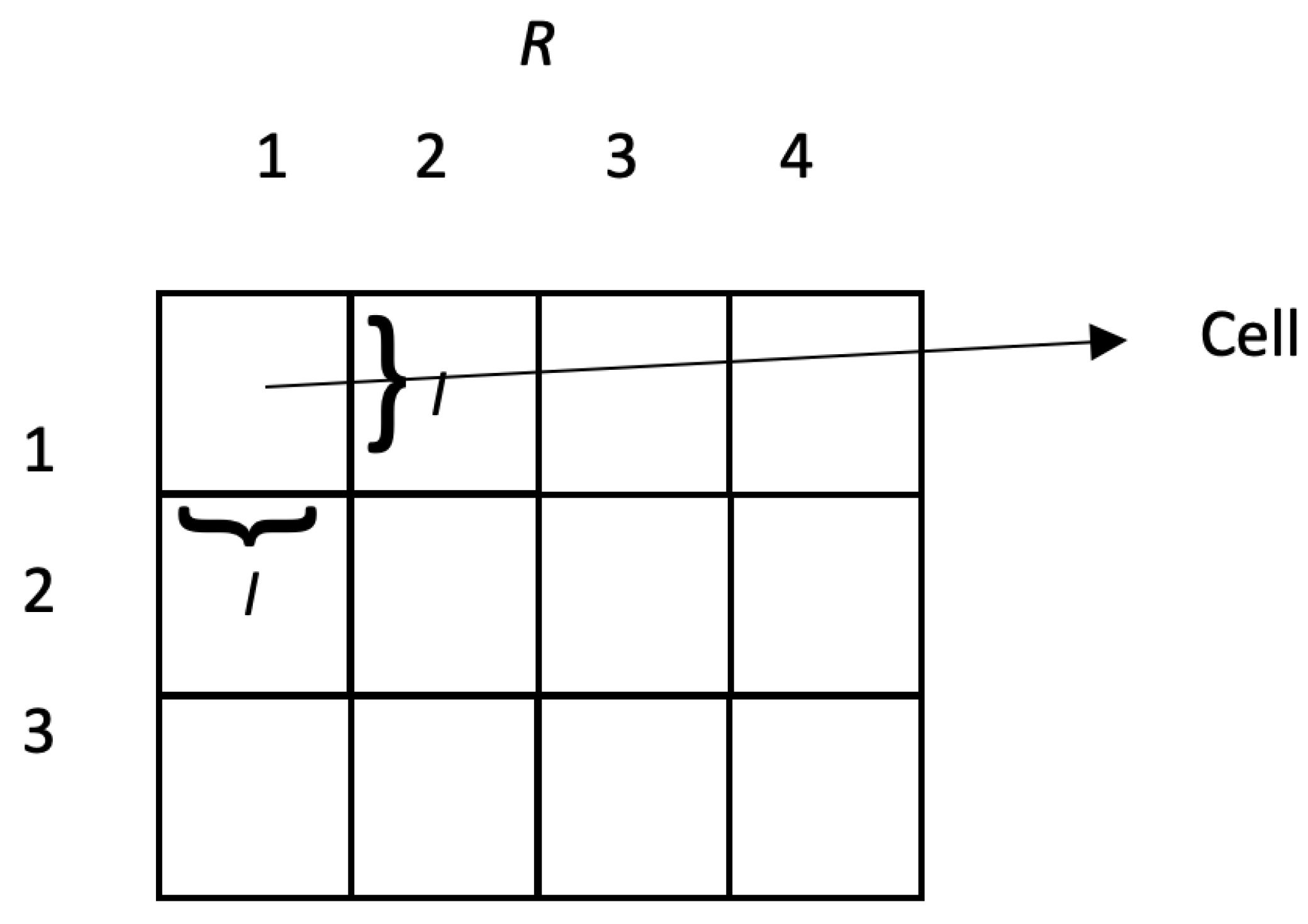
Spatial segmentation: The region of interest (i.e., the geographical space) is segmented into cells (square tessellation, square tiling) of side l, l ∈ I+ (positive integers). The region of interest is represented by a bidimensional array R of order p × q, p, q ∈ I+. The element R[v, w], 0 < vp, 0 < wq, v, w ∈ I+; corresponds to a cell. We assume that the neighborhood relationships between the cells in the real world correspond to those established in the array R (according to rows and columns). Thus, e.g., the adjacent cells of the cell R[1, 1] are R[1, 2] (on the right), R[2, 1] (on the bottom), and R[2, 2] (diagonally). Figure 2 shows a region (array of order 3 × 4).
Spatiotemporal scenario: A spatiotemporal scenario STS is a 2-tuple (R, TempSeg) where R is a segmented region and TempSeg is a temporal segment.
Coordinated Point (CP): A coordinated point is a 3-tuple (x, y, t), x, y ∈ R+, t is a timestamp, where x represents the latitude, y the longitude, and t the time when the CP was generated. For example, (10, 20, ‘15 June 2022 13:30:00’) is a CP.
Trajectory: A trajectory T is a sequence of n CPs, n ∈ I+, T = <(x1, y1, t1), (x2, y2, t2), …, (xn, yn, tn)> where ∀i, j ∈ I+: 0 < i < n, 1 < jn, i < j, ti < tj, i.e., the CPs are ordered temporally (by the ascending time of the CPs).
Segment of a trajectory in a cell of a spatiotemporal scenario: let us consider:
  • A spatiotemporal scenario STS(R, TempSeg) where R is a region of order p × q.
  • A trajectory T = < (x1, y1, t1), (x2, y2, t2), …, (xn, yn, tn)>.
  • A subtrajectory Subt of T, Subt = < (xj, yj, tj), (xj+1, yj+1, tj+1), …, (xj+m, yj+m, tj+m)>, 0 < j < n, m ∈ I+, (j + m) ≤ n, i.e., |Subt| > 1 (i.e., Subt has at least two CPs). That is, a subtrajectory is a subsequence of at least two CPs of a trajectory.
We say that Subt is a segment of T in R[v, w] (R[v, w] is a cell of STS), 0 < vp, 0 < wq, if it meets the following conditions:
(a)
∀ CP (xk, yk, tk) ∈ Subt, k ∈ I+, jk ≤ (j+m), (xk, yk) is inside R[v, w], i.e., the cell R[v, w] contains the CP (xk, yk, tk) (spatial inclusion [21]).
(b)
∀ CP (xk, yk, tk) ∈ Subt, k ∈ I+, jk ≤ (j+m), tkTempSeg, i.e., the segment TempSeg includes the CP (xk, yk, tk) (temporal inclusion [22]).
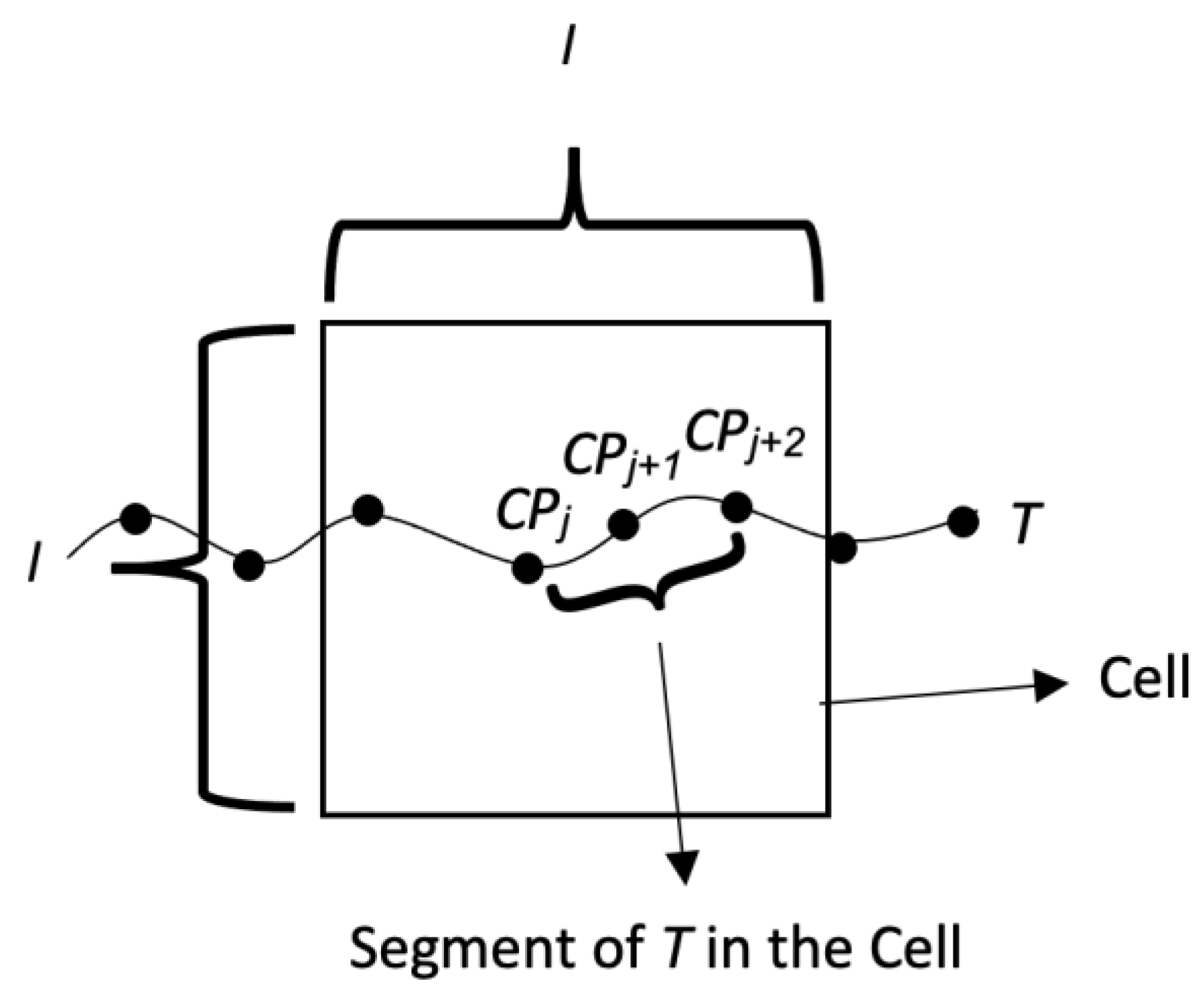
Informally, condition (a) guarantees the spatial inclusion of all the CPs of the segment Subt in the cell R[v, w] and condition (b) in turn, guarantees the temporal inclusion of all the CPs of the segment Subt in the temporal segment TempSeg. Figure 3 shows a segment of T in a cell of a spatiotemporal scenario.
We say that Subt is a maximal segment in R[v, w] if, in addition to conditions (a) and (b), it meets the following:
(c)
The first CP of Subt, i.e., (xj, yj, tj), is the first CP of T (i.e., j = 1), or if j > 1 then, (xj-1, yj-1) is not inside R[v, w] or tj-1TempSeg.
(d)
The last CP, i.e., (xj+m, yj+m, tj+m), of Subt is the last CP of T (i.e., j + m = n), or if j+m < n then: (xj+m+1, y j+m+1) is not inside R[v, w] or tj+m+1TempSeg.
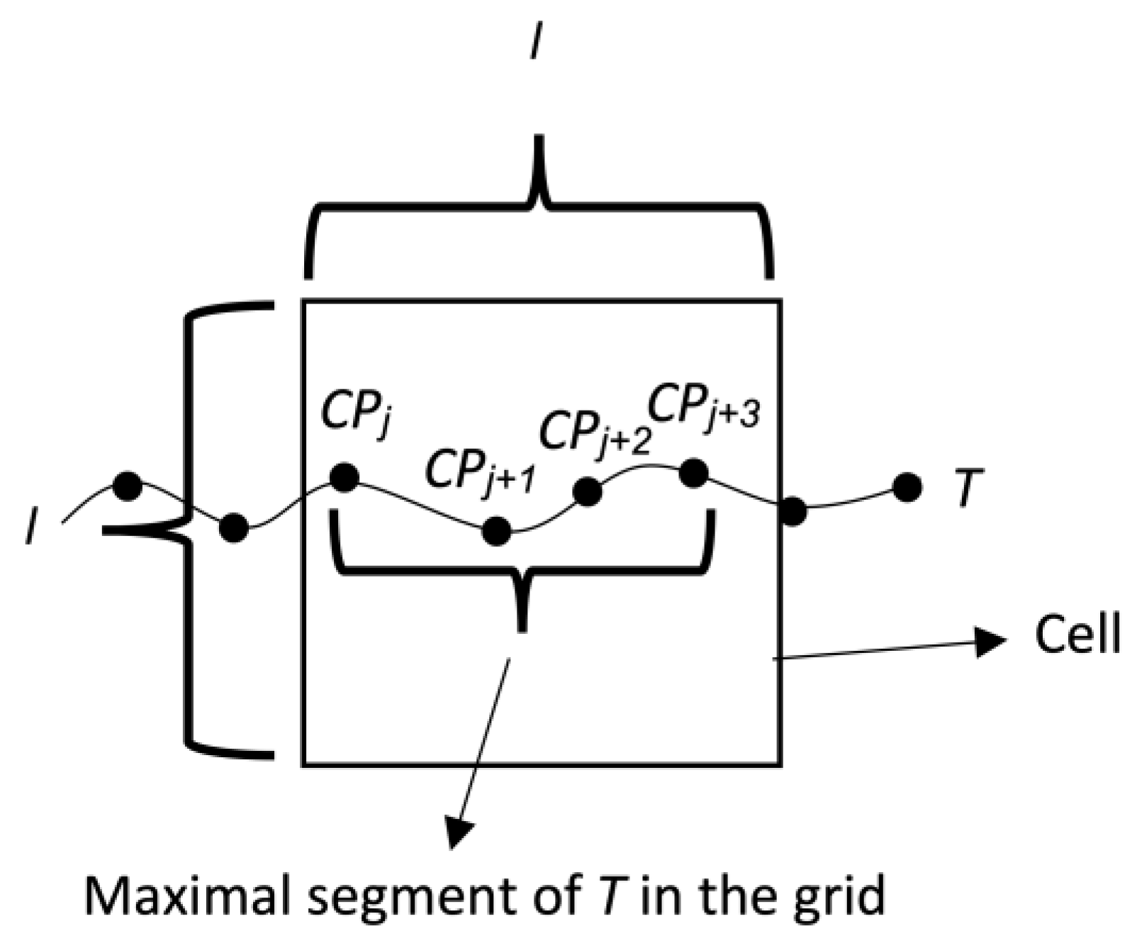
In this way, conditions (c) and (d) guarantee that Subt is the segment of the maximum size with respect to conditions (a) and (b). Figure 4 illustrates a maximal segment of T in a cell of a spatiotemporal scenario.
On the other hand, let Subt = < (xj, yj, tj), (xj+1, yj+1, tj+1), …, (xj+m, yj+m, tj+m) > a segment of T in R[v, w]. We say that Subt is a slow segment in R[v, w] if, in addition to conditions (a) and (b), it meets the following:
(e)
Let MaxSpeed be a speed limit set by the analyst, where MaxSpeed ∈ R+, then ∀ (xk, yk, tk) and (xk+1, yk+1, tk+1), k ∈ I+, jk < (j + m), i.e., for every pair of consecutive CPs in Subt, their speed (calculated as the distance of the straight line between (xk, yk) and (xk+1, yk+1) divided by (tk+1- tk)) is less than or equal to MaxSpeed.
Moreover, a slow segment is maximal if it meets the following:
(f)
The first CP of Subt, i.e., (xj, yj, tj), is the first CP of T (i.e., j = 1), or if j > 1 then, the speed between (xj-1, yj-1, tj-1) and (xj, yj, tj) is greater than MaxSpeed, or (xj-1, yj-1) is not inside R[v, w], or tkTempSeg.
(g)
The last CP of Subt, i.e., (xj+m, yj+m, tj+m), is the last CP of T(i.e., j+m = n), or if j+m < n then, the speed between (xj+m, yj+m, tj+m) and (xj+m+1, yj+m+1, tj+m+1) is greater than MaxSpeed, or (xj+m+1, yj+m+1) is not inside R[v, w] or tj+m+1TempSeg.
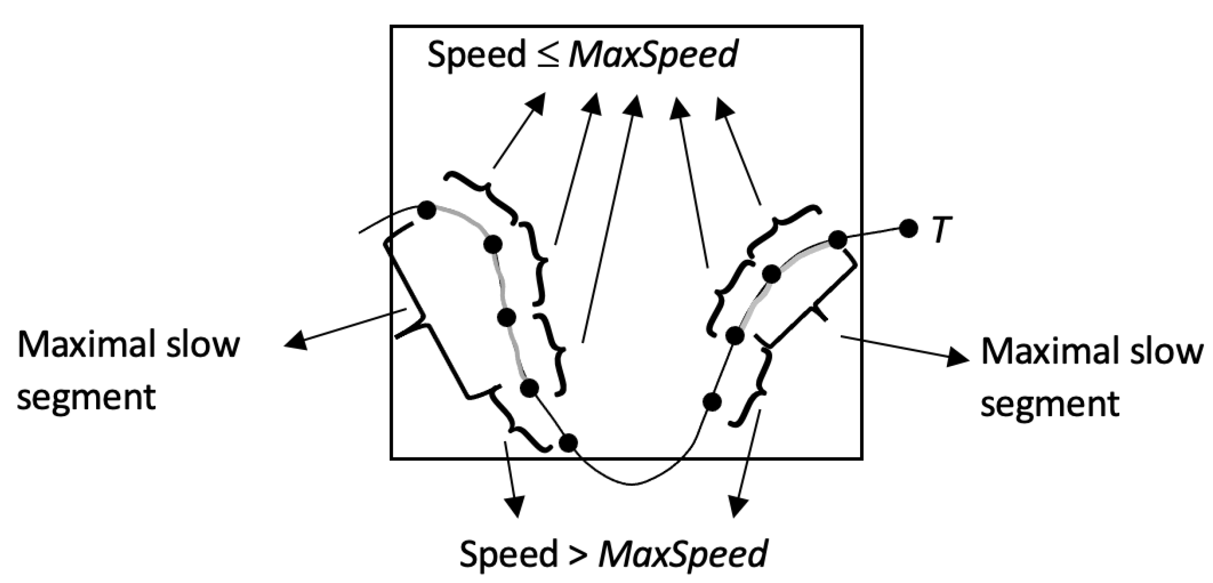
Informally, condition (e) guarantees that the speed among all the consecutive CPs of a slow segment is less than the given speed limit (MaxSpeed). Meanwhile, conditions (f) and (g) guarantee that a slow segment has the maximum cardinality (i.e., the number of CPs) with respect to conditions (a), (b), and (e). Figure 5 shows a trajectory with two maximal slow segments in a cell of a spatiotemporal scenario.
In Table 1 we summarize our segment types in a cell (R[v, w]) and the conditions that each must meet.
Speed limit rate in a cell of a spatiotemporal scenario: Let R[v, w] be a cell of a spatiotemporal scenario STS(R, TempSeg) where R is a region of order p × q, 0 < vp; 0 < wq, v, w ∈ I+, MaxSlowSeg = {mss1, mss2, …, mssp} the set of all the maximal slow segments of all the trajectories that passed through R[v, w], and MaxSeg = {ms1, ms2, …, msk} the set of all the maximal segments of all the trajectories that passed through R[v, w]. The speed limit rate of R[v, w] is given by Equation (1).
Speed   limit   rate = i = 0 p segmentDistance ( m s s i ) , m s s i     M a x S l o w S e g i = 0 k segmentDistance ( m s i ) , m s s i     M a x S e g
where the segmentDistance(s) function calculates the length of a segment s, i.e., the sum of the distances of the consecutive CPs of s, see Equation (2). We calculate the distance between two consecutive CPs using the Euclidean distance formula. Thus, given a segment s = <(xj, yj, tj), (xj+1, yj+1, tj+1), …, (xj+m, yj+m, tj+m)> then:
segmentDistance ( s ) = k = j j + m 1 EuclideanDistance ( ( x k ,   y k ) ,   ( x k + 1 ,   y k + 1 ) )
where EuclideanDistance((xk, yk), (xk+1, yk+1)) = SQRT((xk+1xk)2 + (yk+1yk)2)
Note that in Equation (1), the numerator corresponds to the total distance of all the maximal slow segments and the denominator corresponds to the total distance of all the maximal segments.
Example:
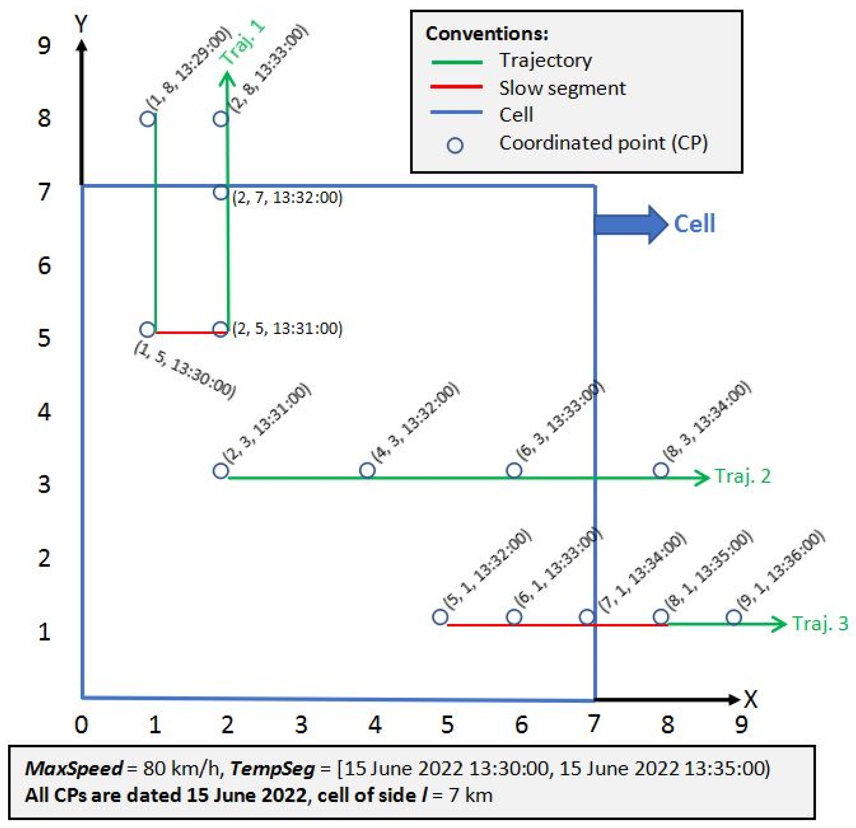
Consider Figure 6, where we show a cell of side l = 7 km of a spatiotemporal scenario, three trajectories corresponding to three vehicles, and TempSeg = [15 June 2022 13:30:00, 15 June 2022 13:35:00). For simplicity, we use a Cartesian coordinate system. If coordinates are in a different coordinate system, e.g., GNSS (global navigation satellite systems) coordinates, a transformation is required, as we have explained in our experiments.
From Figure 6, we have:
MaxSeg = {ms1, ms2, ms3} = {
<(1, 5, 15 June 2022 13:30:00), (2, 5, 15 June 2022 13:31:00), (2, 7, 15 June 2022 13:32:00)>,
<(2, 3, 15 June 2022 13:31:00), (4, 3, 15 June 2022 13:32:00), (6, 3, 15 June 2022 13:33:00)>,
<(5, 1, 15 June 2022 13:32:00), (6, 1, 15 June 2022 13:33:00), (7, 1, 15 June 2022 13:34:00)>
}
Note that in ms2, we do not include the point (7, 3) because we do not have the time when it was generated, i.e., it is an incomplete CP (in future work, its time may be interpolated).
Thus:
segmentDistance(ms1) = 1 + 2 = 3 km
segmentDistance(ms2) = 2 + 2 = 4 km
segmentDistance(ms3) = 1 + 1 = 2 km
Then, the total distance of all the maximal segments is 3 + 4 + 2 = 9 km (denominator in Equation (1)).
MaxSlowSeg = {mss1, mss2} = {
<(1, 5, 15 June 2022 13:30:00), (2, 5, 15 June 2022 13:31:00)>,
<(5, 1, 15 June 2022 13:32:00), (6, 1, 15 June 2022 13:33:00), (7, 1, 15 June 2022 13:34:00)>
}
For example, the segment mss1 is a maximal slow segment because the speed between its two CPs is:
EuclideanDistance((1, 5), (2, 5)) = SQRT((2 − 1)2 + (5 − 5)2) = 1 km.
Time between the two CPs = 1 min.
Thus, speed = 1 km/min = 60 km/h, and because MaxSpeed = 80 km/h, then, 60 km/h ≤ 80 km/h. Note that the speed between (2, 5, 15 June 2022 13:31:00) and (2, 7, 15 June 2022 13:32:00) is 2 km/min = 120 km/h and 120 km/h > 80 km/h.
Thus:
segmentDistance(mss1) = 1 km.
segmentDistance(mss2) = 1 + 1 = 2 km.
Then, the total distance of all the maximal slow segments is 1 + 2 = 3 km (numerator in Equation (1)).
Therefore:
Speed limit rate = 3/9 = 0.333.
The CellSpeedLimitRate algorithm finds the speed limit rate of a cell of a spatiotemporal scenario. It receives a set of trajectories (TT), a cell (r), a speed limit (MaxSpeed), and the temporal segment (TempSeg) associated with the spatiotemporal scenario where the cell r is located.
CellSpeedLimitRate(TT, r, MaxSpeed, TempSeg)
Input:
TT //Array of trajectories
r //Cell of a spatiotemporal scenario where the speed limit rate will be computed
MaxSpeed //Speed limit
TempSeg //Temporal segment of the spatiotemporal scenario where the cell r is located
Output:
speedLimitRate //Speed limit rate of r
DECLARE
speedLimitRate = 0;
maximalSlowSegmentsDistance = 0; //Total distance of all the maximal slow segments
maximalSegmentsDistance = 0; //Total distance of all the maximal segments
euclideanDist; //Euclidean distance between two CPs
BEGIN
1. FOR EACH trajectory T ∈ TT
2.     //Traverse trajectory T
3.     FOR i = 1 TO size(T)-1; //size(T) function returns the number of CPs of T
4.       //Check spatial and temporal inclusion of T[i] and T[i+1] in r
5.       IF (inside((T[i].x, T[i].y), r) AND T[i].t ∈ TempSeg AND
6.                 inside((T[i+1].x, T[i+1].y), r) AND T[i+1].t ∈ TempSeg) THEN
7.           //Euclidean distance between T[i] and T[i+1]
8.                 euclideanDist = euclideandistance((T[i].x, T[i].y), (T[i+1].x, T[i+1].y))
9.                 maximalSegmentsDistance += euclideanDist;
10.           //Checks the speed condition
11.               IF (speed(T[i], T[i+1]) MaxSpeed) THEN
12.                     maximalSlowSegmentsDistance += euclideanDist;
13.             END IF
14.       END IF
15.     END FOR
16. END FOR EACH
17. IF (maximalSegmentsDistance > 0) THEN
18.           //Compute speed limit rate of r
19.           speedLimitRate = maximalSlowSegmentsDistance / maximalSegmentsDistance;
20. END IF;
21. RETURN speedLimitRate;
END CellSpeedLimitRate
Basically, the algorithm loops through the array of trajectories TT (line 1). Next, the CPs of each trajectory T (line 3) are traversed. For each pair of consecutive CPs, T[i] and T[i+1] are verified if both are inside cell r (spatial inclusion) and belong to the temporal segment TempSeg (temporal inclusion) (lines 5 and 6). If so, the variable maximalSegmentsDistance (line 9) is incremented and then it is verified if the two CPs also meet the speed condition (line 11). If so, the variable maximalSlowSegmentsDistance (line 12) is incremented. Finally, the algorithm computes the speedLimitRate (line 19). Note that each trajectory is traversed only once. Thus, the total number of iterations of the algorithm is equal to the total number of CPs of the trajectories—|TT| (because the last CP of each trajectory is not traversed, see line 3).
The inside(p, r) Boolean function (lines 5 and 6), where p is a point(x, y) and r is a cell (a square of side l), is defined as follows. Let (rx, ry) be the coordinate of the bottom-left corner of r. The function returns TRUE if p is inside r otherwise, it returns FALSE. p is inside r if the two following conditions are met:
  • xrx and xrx + l
  • yry and yry + l
The speed(T[i], T[i+1]) function (line 11) is calculated as follows:
speed(T[i], T[i+1]) = EuclideanDistance((T[i].x, T[i].y), (T[i+1].x, T[i+1].y))/(T[i+1].t − T[i].t).

3. Results and Discussion

The experiments were carried out with public data of taxi trips from Porto (Portugal) and its surrounding areas [23]. Each data packet corresponds to a completed trip (a taxi trajectory). These taxis operate through a taxi dispatch center, using mobile data terminals installed in the vehicles. Each data packet of a taxi trajectory includes (among other data):
  • TRIP_ID: trip identifier.
  • TAXI_ID: taxi id.
  • TIMESTAMP: time when the trip began.
  • POLYLINE: list of coordinates [longitude, latitude]. A pair of consecutive coordinates corresponds to 15 s of a trip. The last coordinate corresponds to the trip’s destination, while the first one represents its start.
  • MISSING_DATA: type of the data packet. MISSING_DATA may take two values:
    FALSE: if there are no missing coordinates.
    TRUE: otherwise.
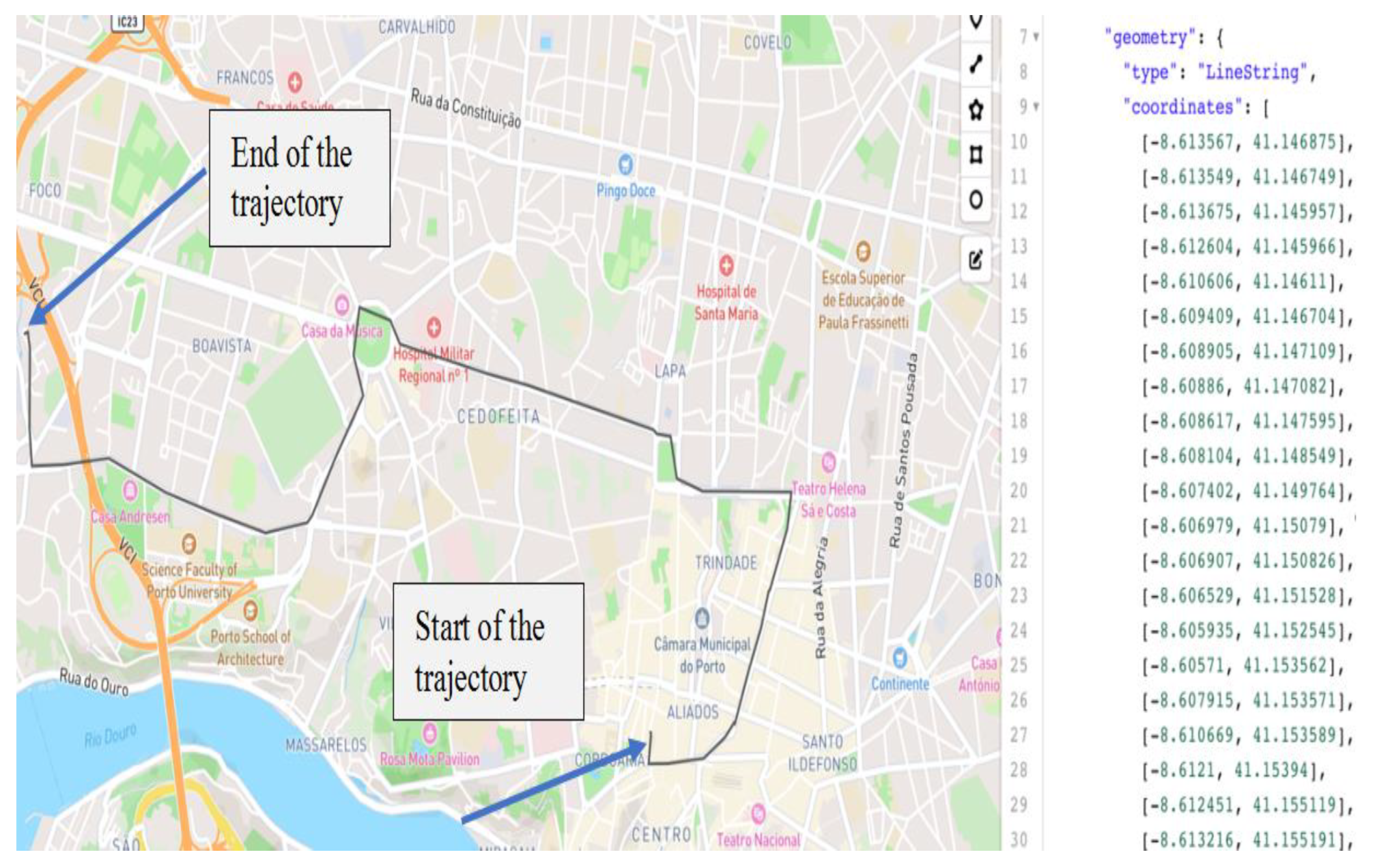
We considered 1048576 trips from 3 August 2013 to 31 August 2013 (28 days), each trajectory had on average 10 coordinates (CPs). The POLYLINE of a trip looks similar to this: [[−8.613567, 41.146875], [−8.613549, 41.146749], [−8.613675, 41.145957], [−8.612604, 41.145966], …, [−8.648334, 41.158017], [−8.648451, 41.15799], [−8.648523, 41.157981]]. In Figure 7, we show this trajectory (we used this tool https://geojson.io, accessed on 30 November 2022).
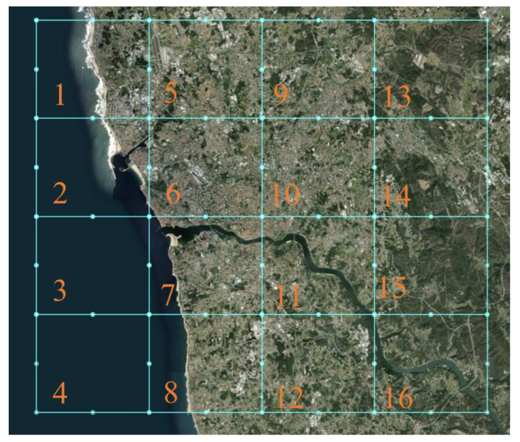
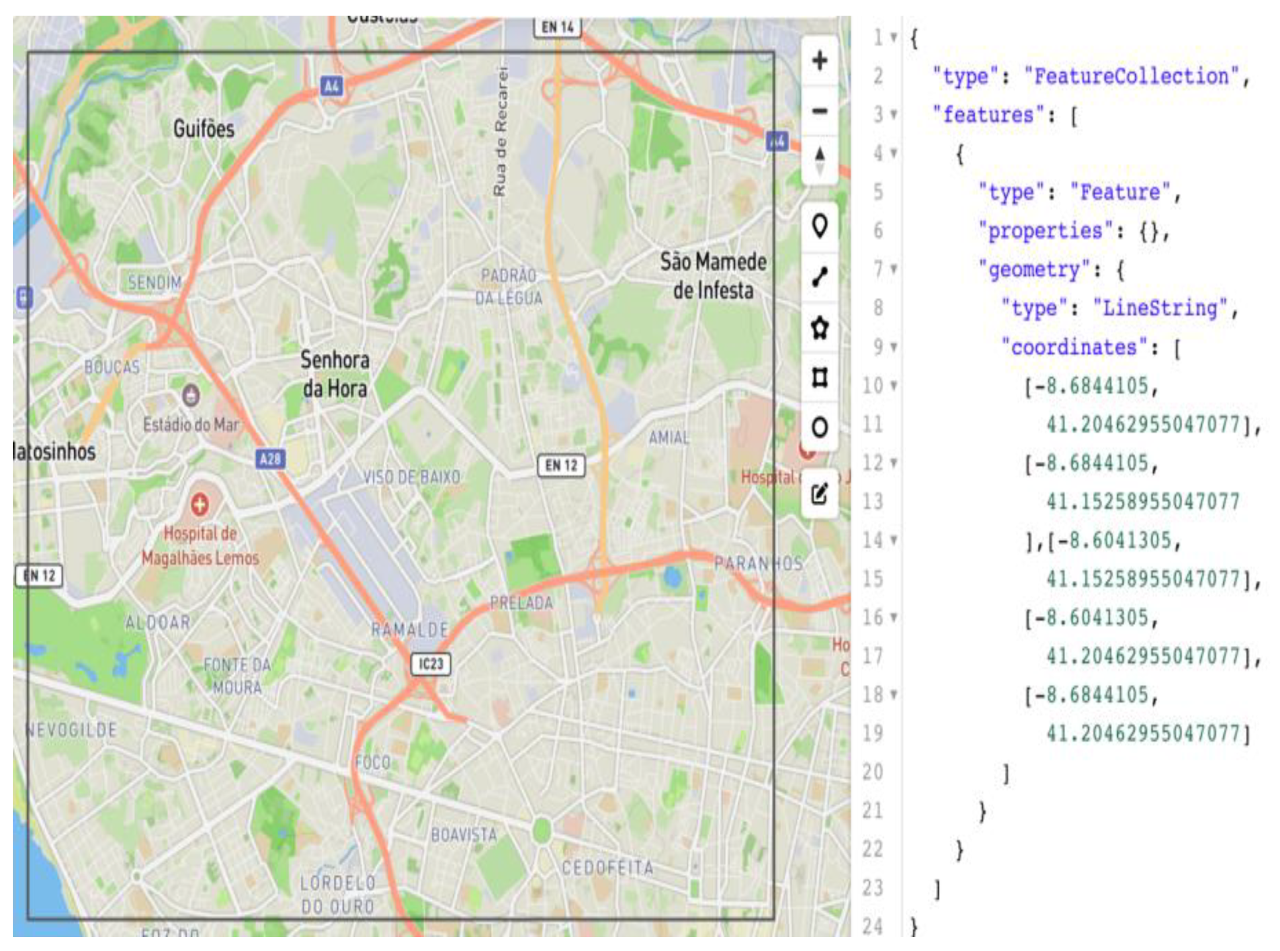
The region of interest, Porto, was segmented into sixteen cells numbered from 1 to 16, see Figure 8. In Figure 9, we detailed cell 6 with its coordinates (note that in Figure 9, in the “coordinates” array, the last coordinate is equal to the first one). To calculate the cell dimensions (km), we used the tool https://www.omnicalculator.com/other/latitude-longitude-distance, accessed on 30 November 2022. One side of the cell measured 5.787 km and the other 6.721 km. As the cell is not a square (it is a rectangle), the inside function of our algorithm was modified in such a way that it verifies the spatial inclusion of a point in a rectangle. We also divided the day into twelve mutually exclusive consecutive temporal segments: (00:00, 02:00], (02:00, 04:00], …, (22:00, 00:00]. Thus, we have 12 spatiotemporal scenarios.
We processed the data, stored in CSV files, with Jupyter Notebook. Before applying our algorithm for computing the speed limit rate, we cleaned the data: we removed repeated data packets and data packets with: (i) the same taxi in different positions at the same time, (ii) missing coordinates, and (iii) excessive speed between two consecutive coordinates (greater than 200 km/h). In addition, we only considered cells of a spatiotemporal scenario with more than 10 trajectories. Note that cells 3 and 4 are located entirely in the ocean; therefore, there are no trajectories passing through these cells.
To compare the results of our speed limit rate measure, we also conducted experiments with the SPI (speed performance index) [19,24], which is an index to measure the traffic state level of a road. SPI = 100*(Vavg/Vmax), where Vavg is the average speed in a cell and Vmax is the maximum permitted speed in the cell. With this index, the traffic state level can be classified as follows: [0, 25) heavy, [25, 50) mild, [50, 75) smooth, and [75, 100] very smooth.
We conducted the following experiments.
  • First: considering the 12 spatiotemporal scenarios and the 14 cells (excluding cells 3 and 4), we ran our algorithm for all the 28 days with MaxSpeed 50 km/h and 40 km/h.
  • Second: from the results of the first experiment, we chose five cells: four of them were the cells with more trajectories, and the other was the one with less trajectories. Then, we ran our algorithm with MaxSpeed values of 50 km/h, 30 km/h, and 10 km/h. For each of these five cells, we obtained the results for 28 days.
  • Third: considering the same five cells as the second experiment, we conducted the corresponding experiments for the SPI with Vmax of 100 km/h, 80 km/h, and 60 km/h.
  • Fourth: analysis of slow segments.

3.1. First Experiment with MaxSpeed 50 km/h and 40 km/h

For the 12 spatiotemporal scenarios, the 14 cells, and the 28 days, we had a total of 14*12*28 = 4704 measurements. In Table 2, we show the results for one day (3 August 2013) with MaxSpeed = 50 km/h and in Table 3, with MaxSpeed = 40 km/h. ND stands for No Data; this means that there were not enough trajectories (less than 11) for a cell in a specific spatiotemporal scenario. Note that all the measurements for cells 3 and 4 are equal to ND. We discuss the results of the first experiment together with those of the second one in the next Section 3.2.
In Table 4, we show the average speed limit rate by day and TempSeg of all the cells.

3.2. Second Experiment

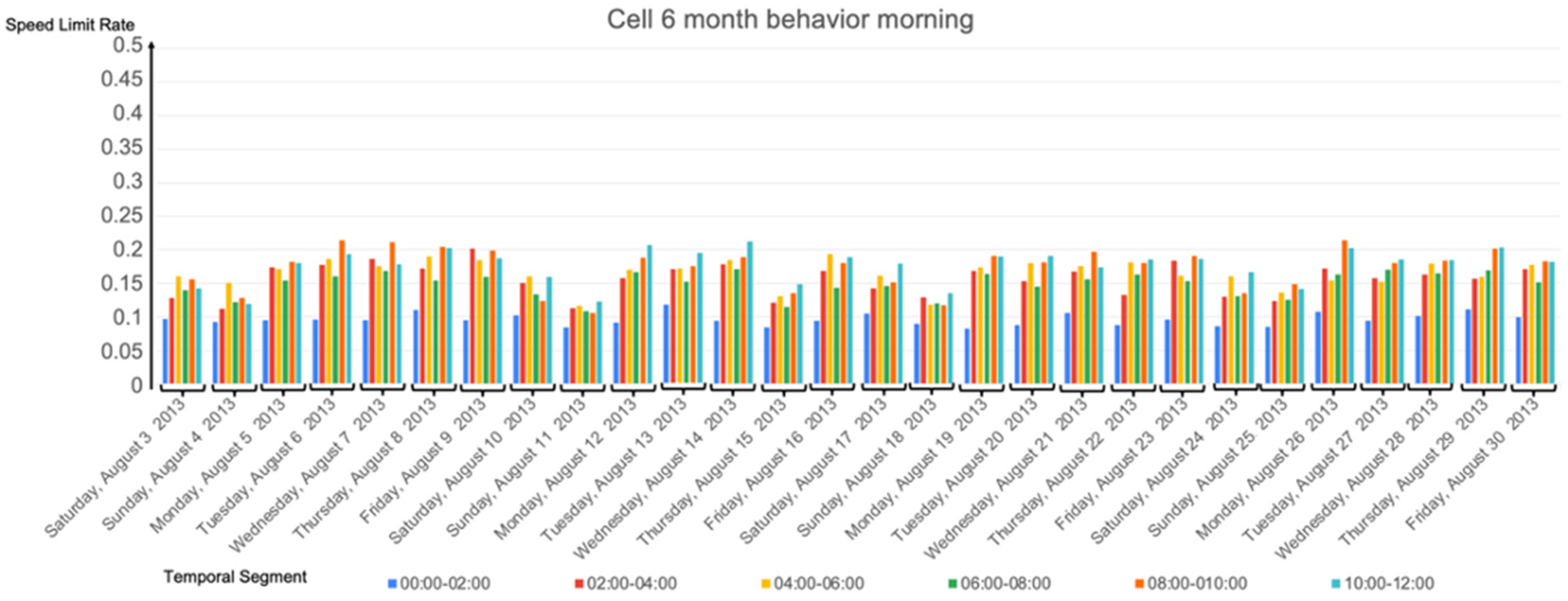
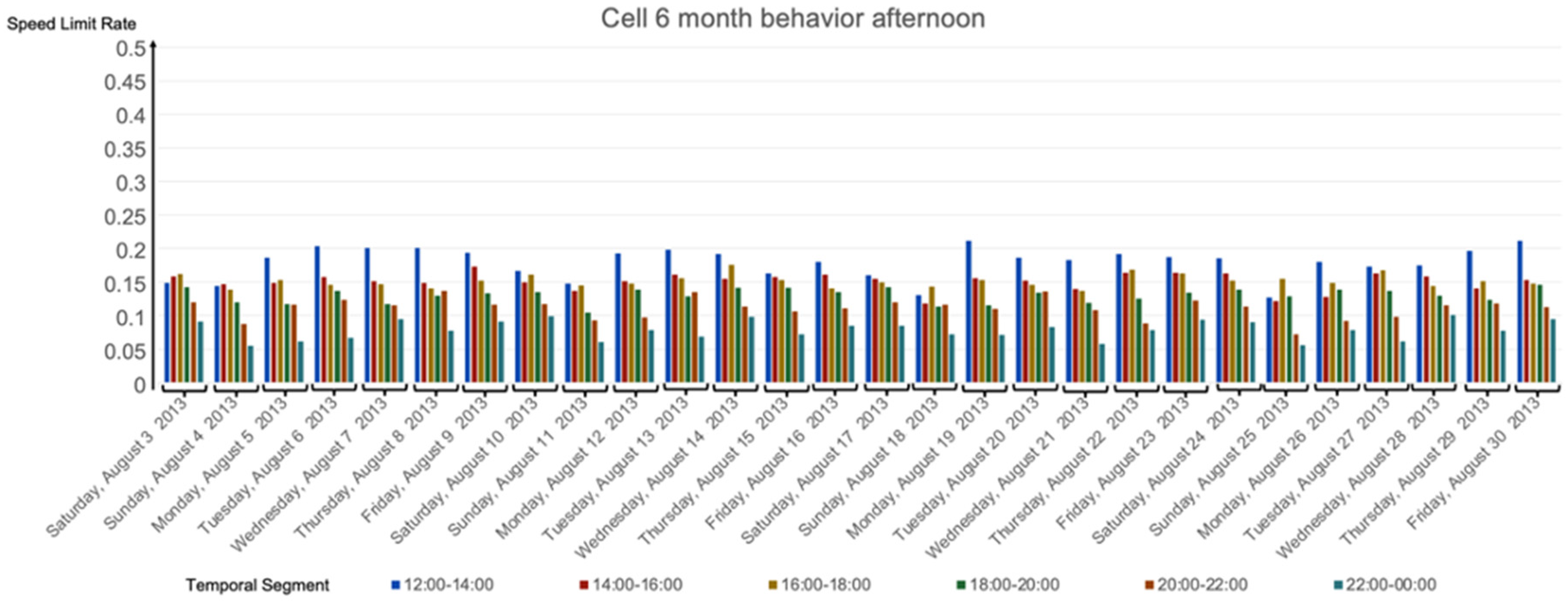
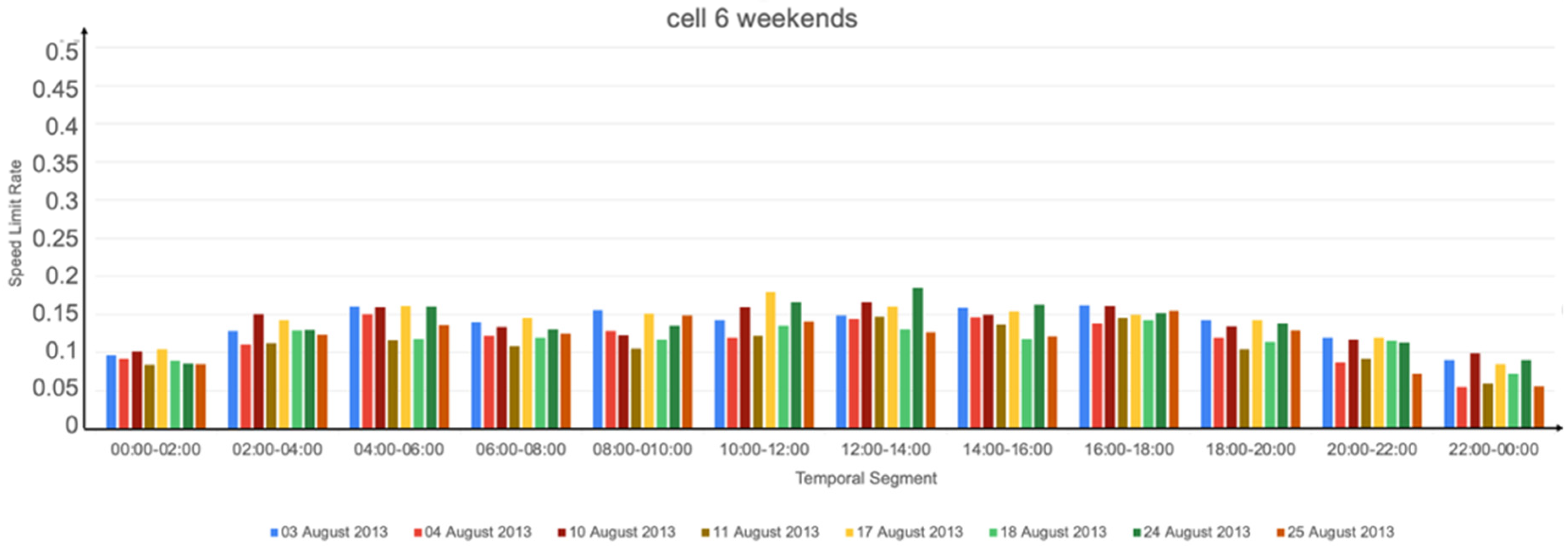
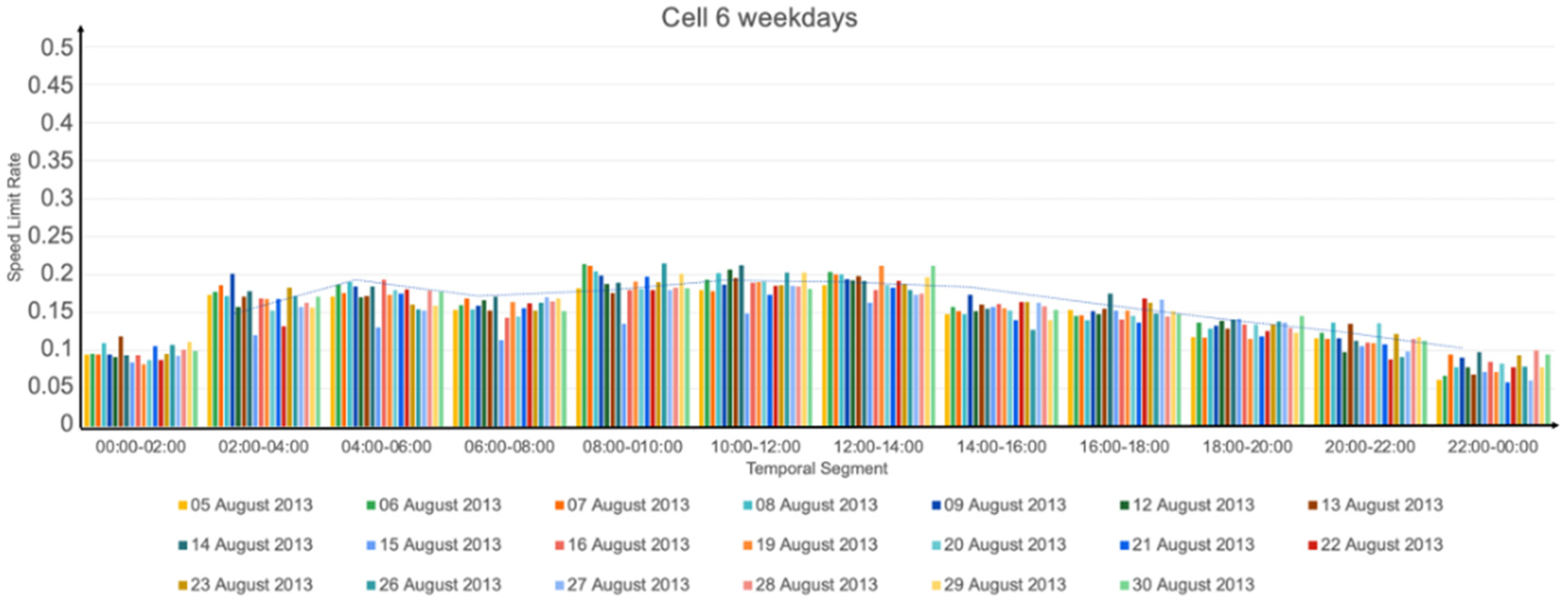
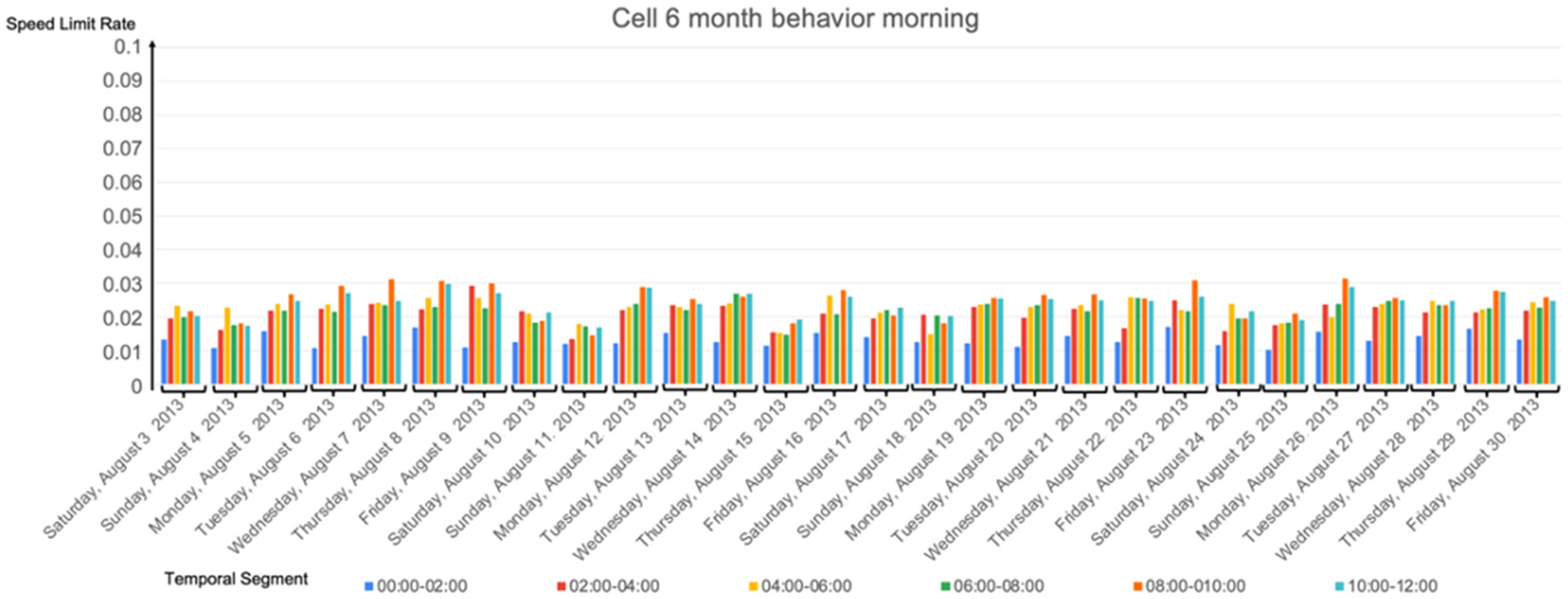
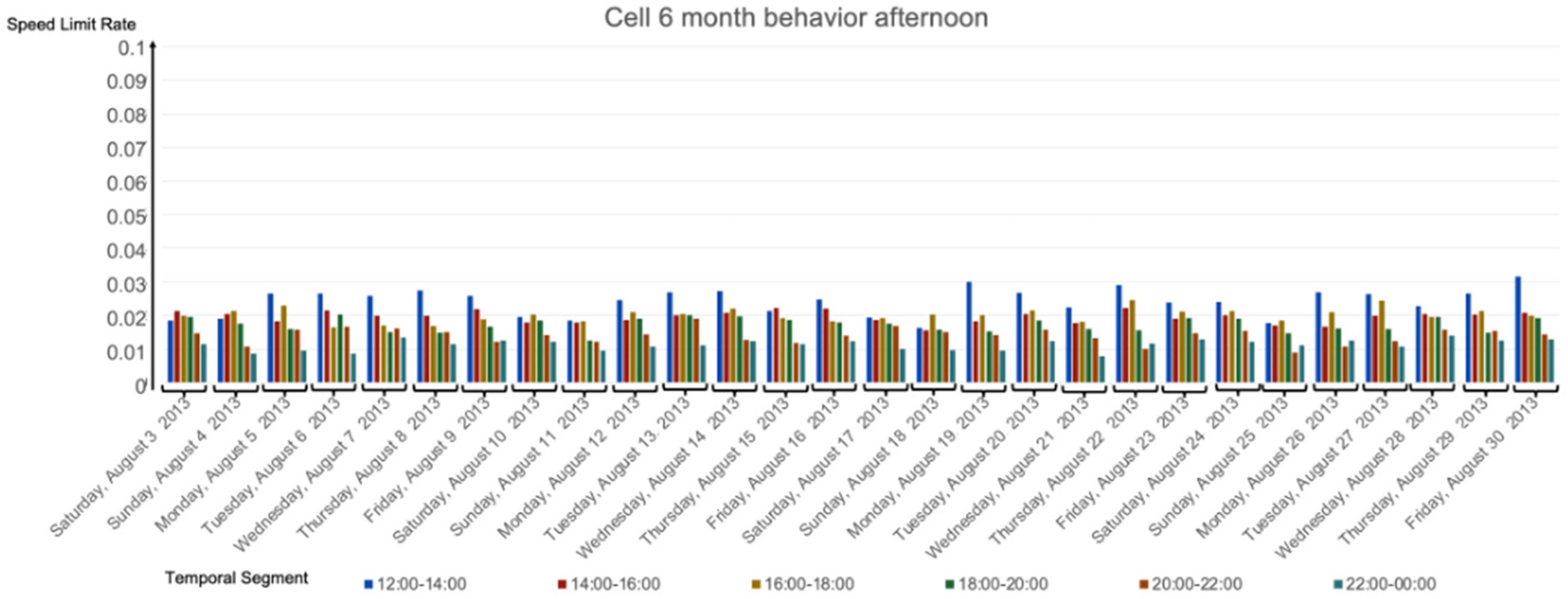
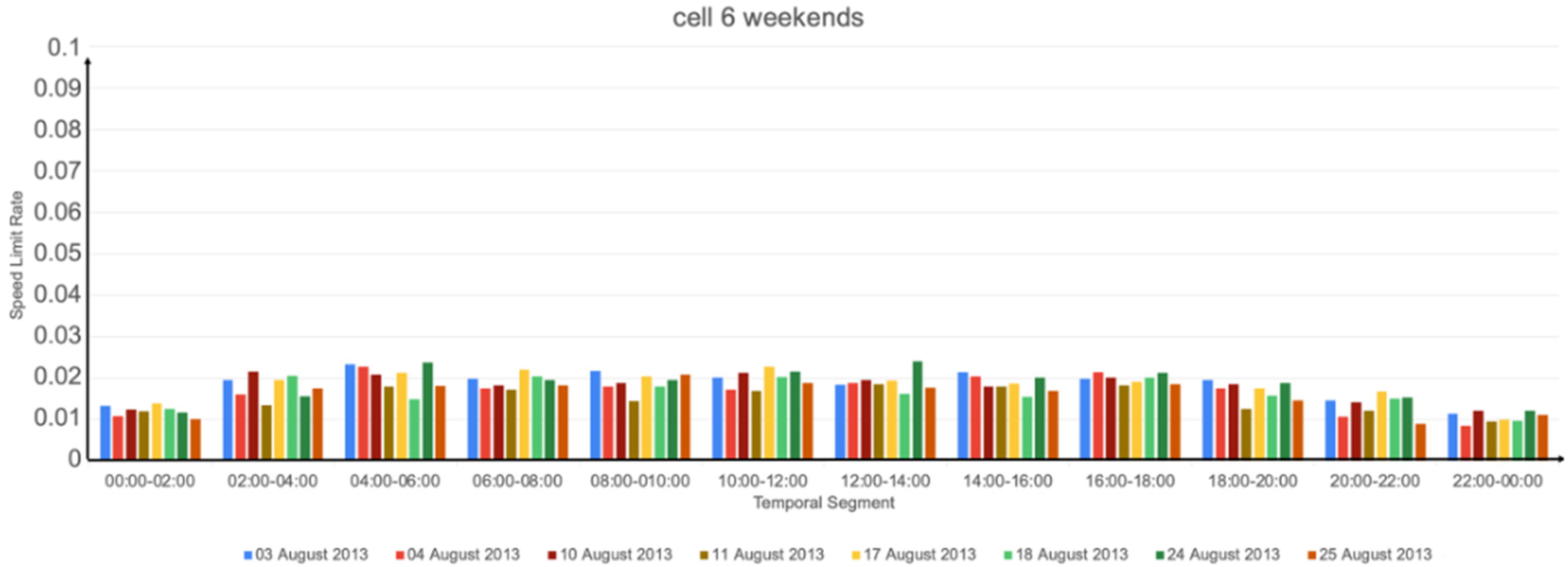
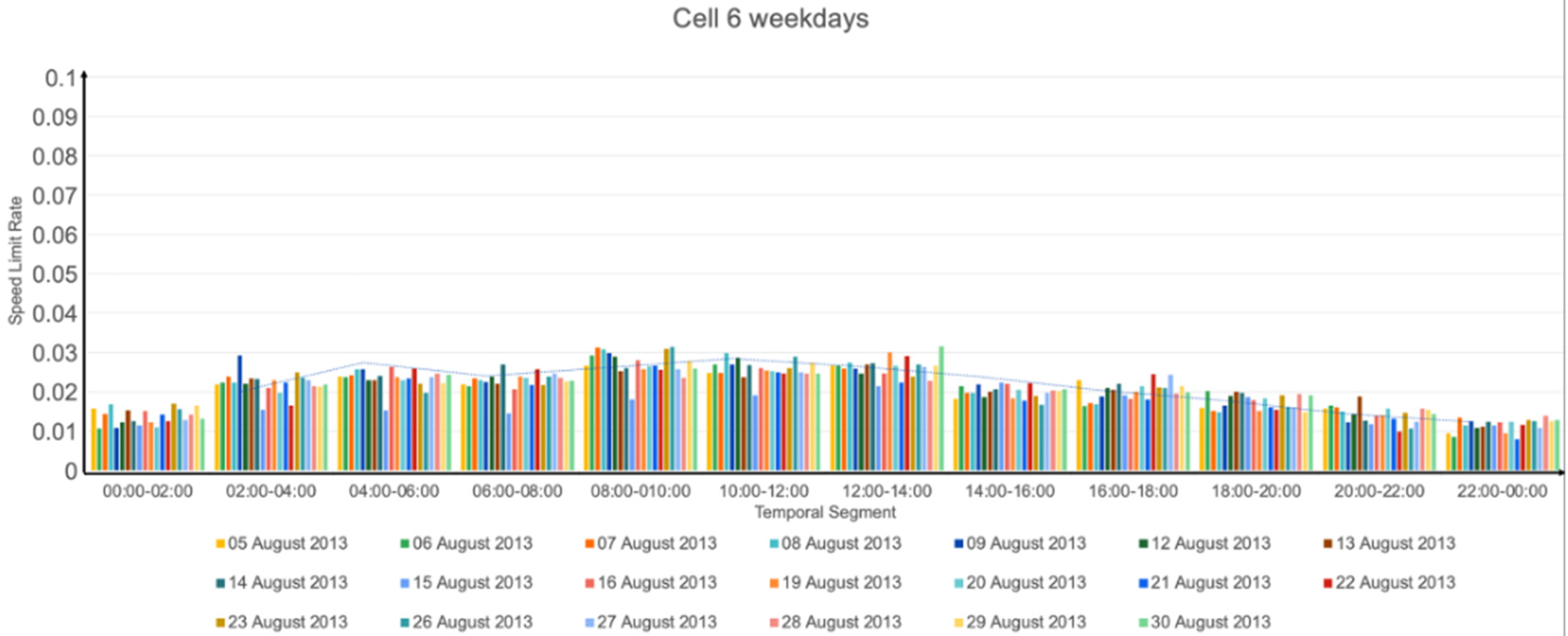
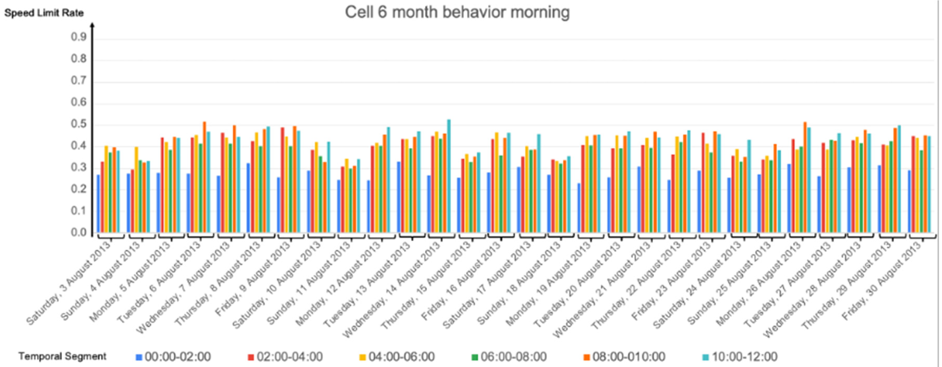
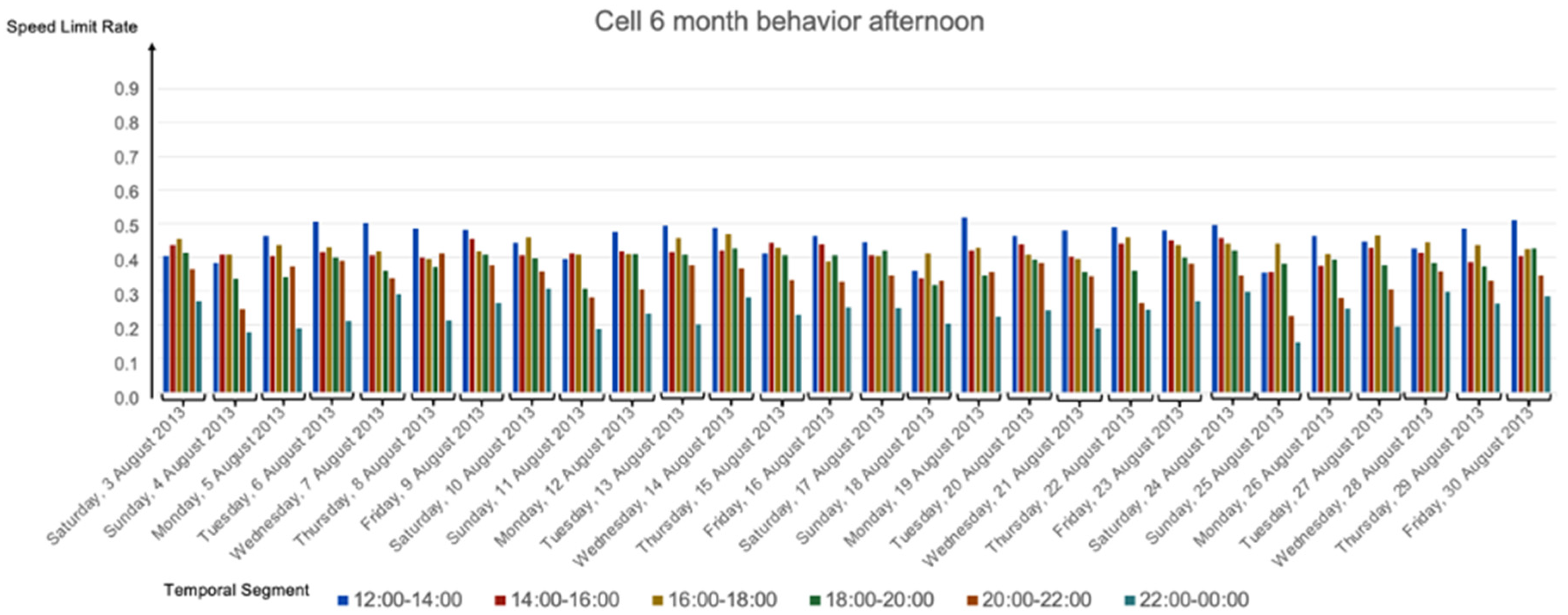
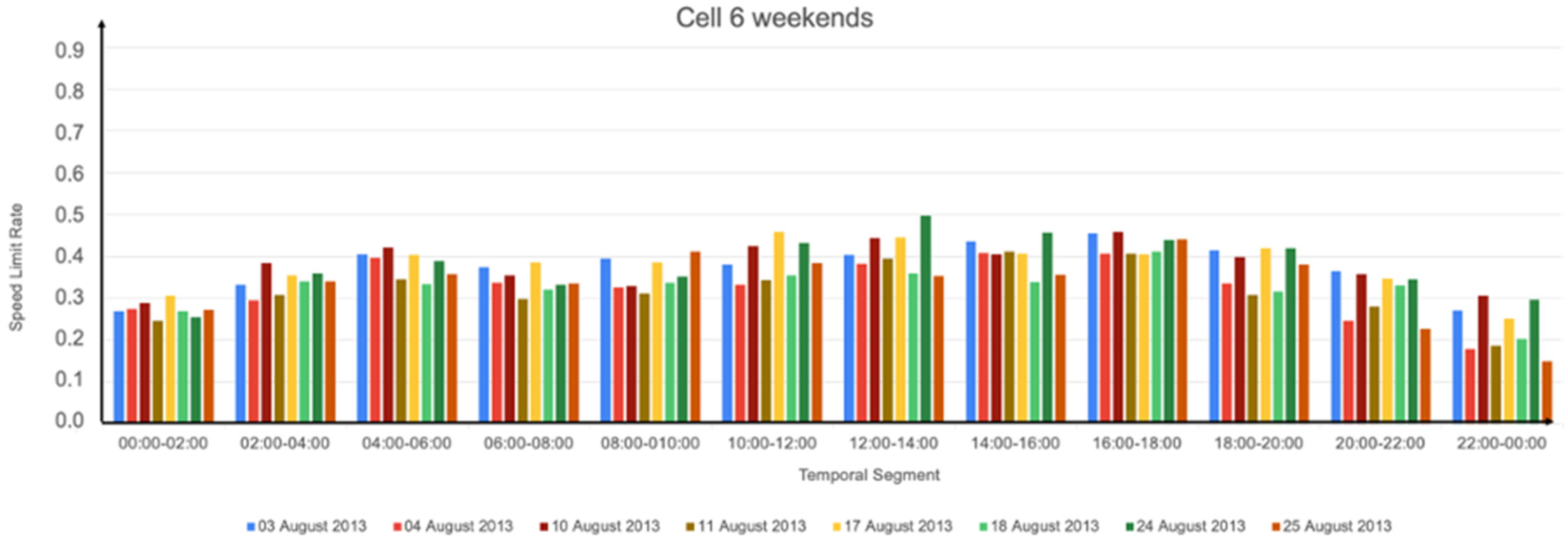
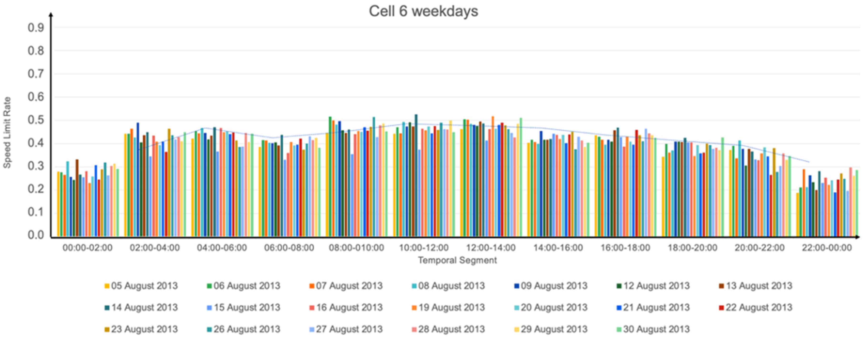
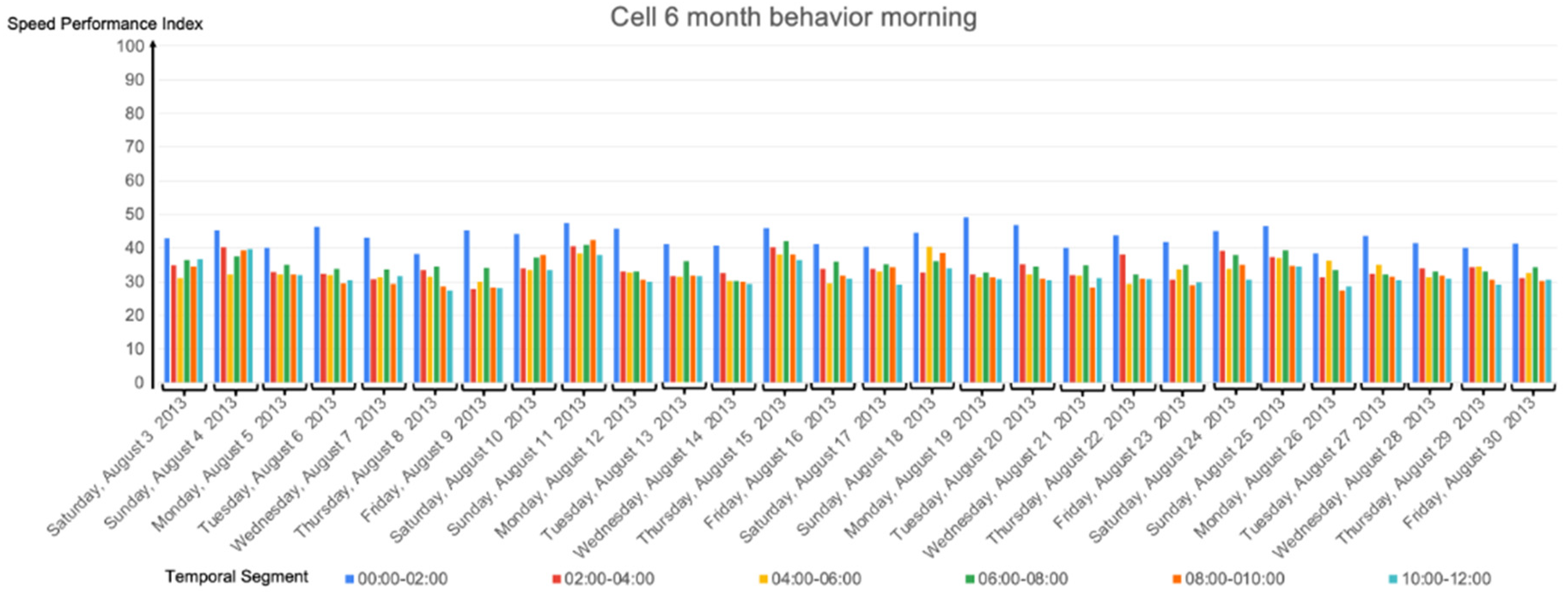
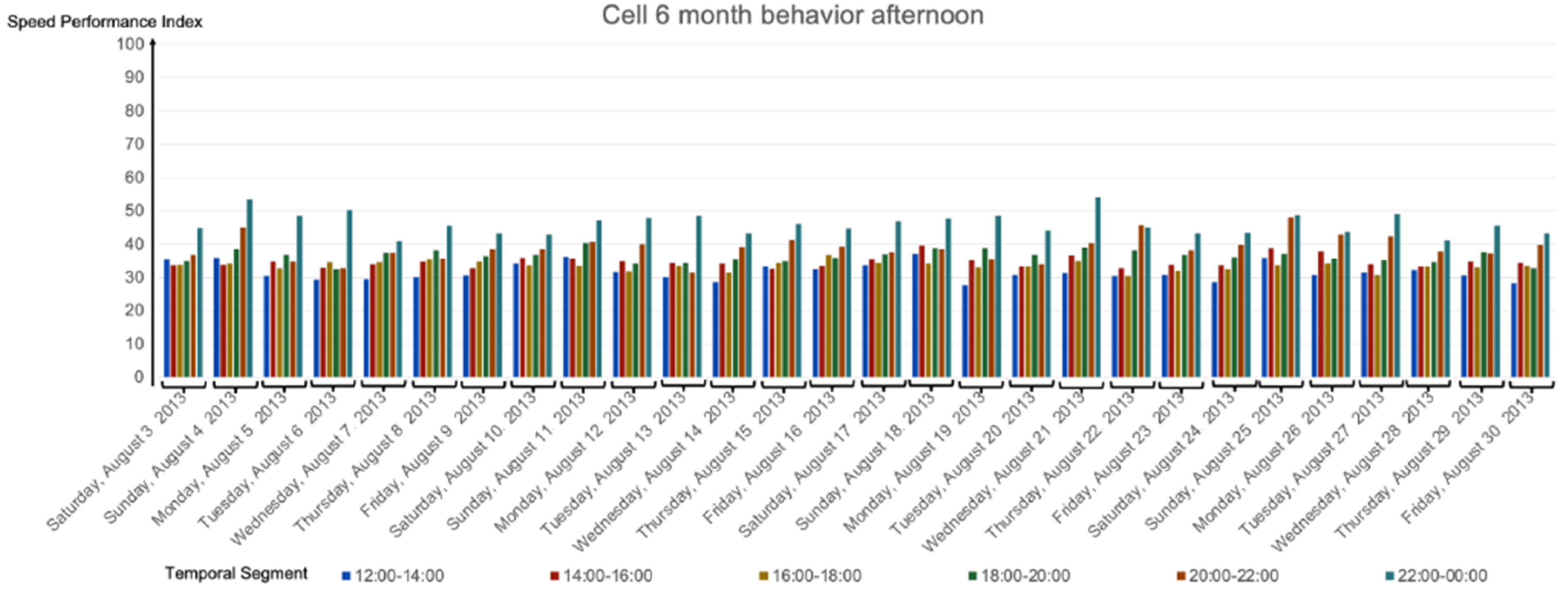
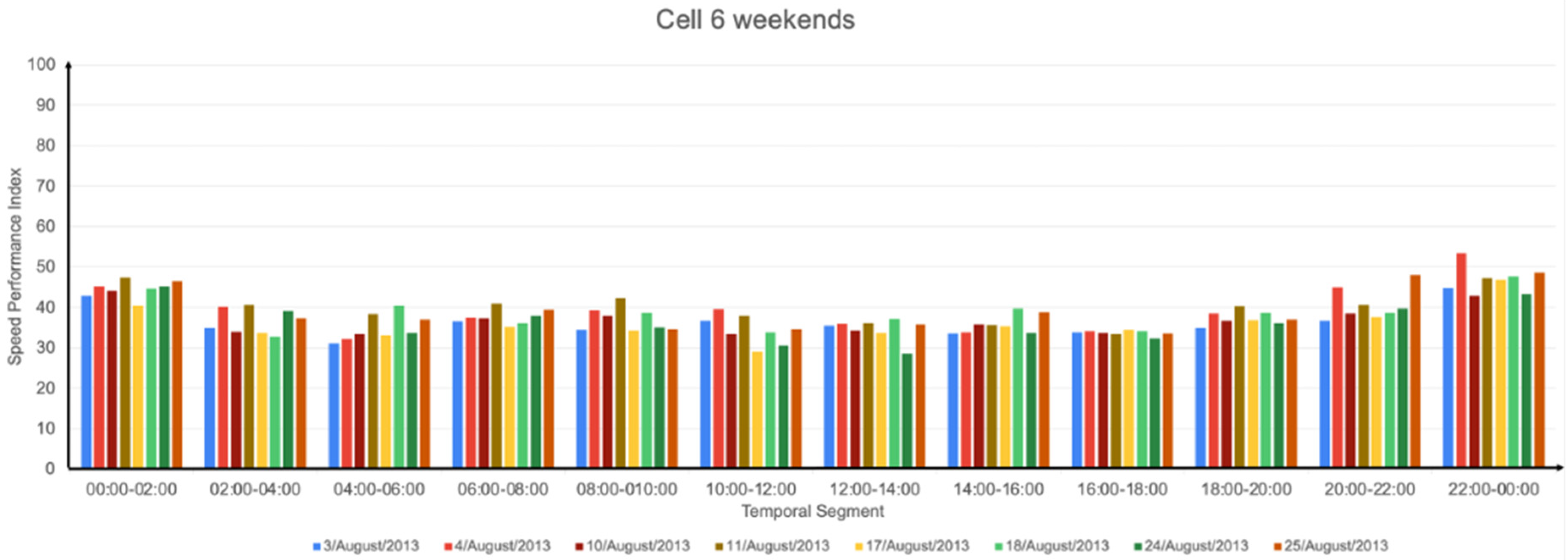
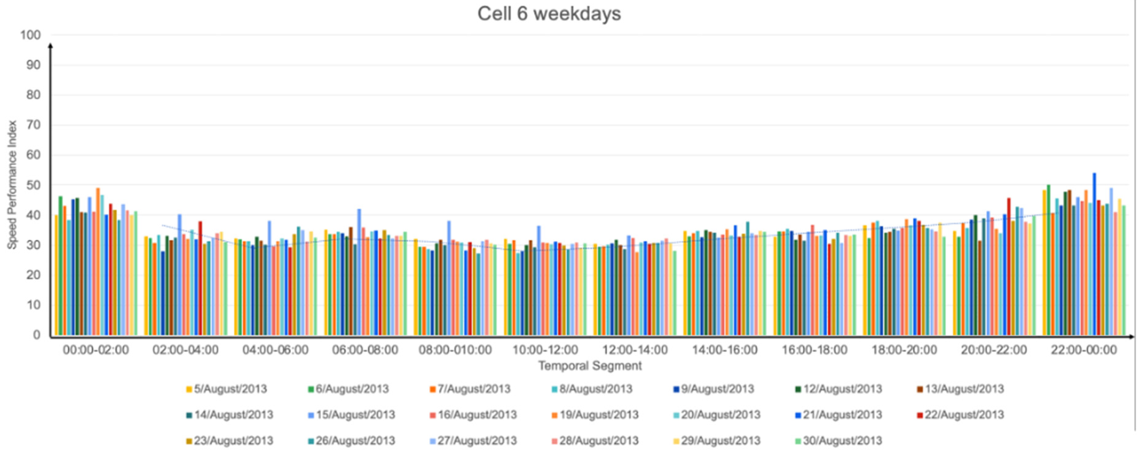
As a result of the two previous experiments, we chose cells 1, 6, 7, 10, and 11 for the next group of experiments. Cells 6, 7, 10, and 11 were the four cells with more trajectories, and cell 1 was the one with fewer trajectories. Then, we ran our algorithm for these five cells. For each cell, we obtained four figures to show the behavior for: (i) 28 days in the morning, (ii) 28 days in the afternoon, (iii) weekends, and (iv) weekdays. Next, we show four figures for cell 6 with MaxSpeed = 50 km/h, Figure 10, Figure 11, Figure 12 and Figure 13. In Appendix A, Figure A1, Figure A2, Figure A3, Figure A4, Figure A5, Figure A6, Figure A7 and Figure A8, we show four figures for cell 6 with MaxSpeed = 30 km/h, and four with MaxSpeed = 10 km/h. In https://drive.google.com/drive/folders/1fMTjd6G1whkFhticrce-EkBWsRWbVCr8?usp=sharing (accessed on 3 December 2022) the reader can access all the figures corresponding to the five cells, with three MaxSpeeds (50, 30, and 10 km/h), and for the 28 days, for the weekends, and for the weekdays. This classification by day of the week allows users to focus their analysis on specific days or groups of days, e.g., to observe if there are recurring behaviors on Fridays or to compare the behavior of Mondays and Sundays.
Considering all the results, first and second experiments, we highlight the following. On average:
  • Weekdays were slower than weekends, especially slower than Sundays in the mornings.
  • Sundays were the slowest days.
  • Mornings and middays (08:00 to 14:00] were slower than the afternoons (14:00 to 20:00] (although, in some cells, e.g., cell 6, the slowness was similar in both time-ranges). This makes sense since in the mornings most people commute to work and school and have lunch at noon. On the other hand, in the afternoons, not all of these people return to their morning activities. Those who do, return home at different times, e.g., in schools, classes usually start at 9:00 and end at 15:30, banks work from 8:30 to 15:00, small stores are open from 9:00 to 18:00, and big stores from 10:00 to 22:00.
  • The temporal segment (08:00, 10:00] was the slowest.
  • The temporal segments (22:00, 00:00] and (00:00, 02:00] were the fastest.
  • There was more slowness between 08:00 and 18:00 than between 18:00 and 08:00.
  • In addition:
  • As MaxSpeed increases, so does the speed limit rate measure in the cells; this is reasonable because as the speed limit increases, more slow segments are generated, and thus, the speed limit rate measure increases as well. Note that, if MaxSpeed → ∞ then speed limit rate = 1, because all the segments that pass through a cell are considered slow.
  • Thursday 15 August 2013 had a “weekend behavior” during the Assumption of Mary, a holiday in Portugal. Note, e.g., in cell 6, Figure 10, Figure A1 and Figure A5, in the morning, had similar results for Thursday 15 August 2013 and Sundays.
  • Considering the five cells of experiment 2, cell 7 was the slowest.
  • (00:00, 02:00], (02:00, 04:00], (20:00, 22:00], and (22:00, 00:00] were the fastest temporal segments. This is reasonable because at these hours, fewer vehicles are circulating.
  • In general, the weekdays had similar behavior, although Mondays tended to be slower than the other weekdays and Tuesdays tended to be faster.

3.3. Third Experiment

Analogously to the second experiment, in Figure 14, Figure 15, Figure 16 and Figure 17 we show the results for cell 6 for the SPI at 100 km/h.
Note that increasing Vmax will change the SPI value proportionally. For example, if in cell 6 between 14:00 and 16:00 on 3 August 2013, Vavg = 50 km/h then, at Vmax = 60, 80, and 100 km/h, we obtain:
SPI = 100 * ( 50 60 )                                   SPI = 100 * ( 50 80 )                 SPI = 100 * ( 50 100 )
SPI = 83.33   SPI = 62.5   SPI   = 50
The results of the SPI were consistent with our speed limit rate measurements: weekdays were a little slower than weekends; on average, Sundays were the slowest days, as were afternoons when compared to mornings, a weekday with an unusual behavior was due to a holiday (Thursday15 August 2013), and extreme time-ranges, (00:00, 02:00], (02:00, 04:00], (20:00, 22:00], and (22:00, 00:00], were the fastest; this makes sense because at extreme time-ranges there is usually less traffic, which makes it easier for vehicles in circulation to move at higher speeds. However, in general, the differences between mornings-middays and afternoons were not greater than 0.2; see, e.g., the peak hours (08:00, 10:00] and (18:00, 20:00] in Table 4, where the speed limit measure ranges in the interval (0.4, 0.6).

3.4. Fourth Experiment

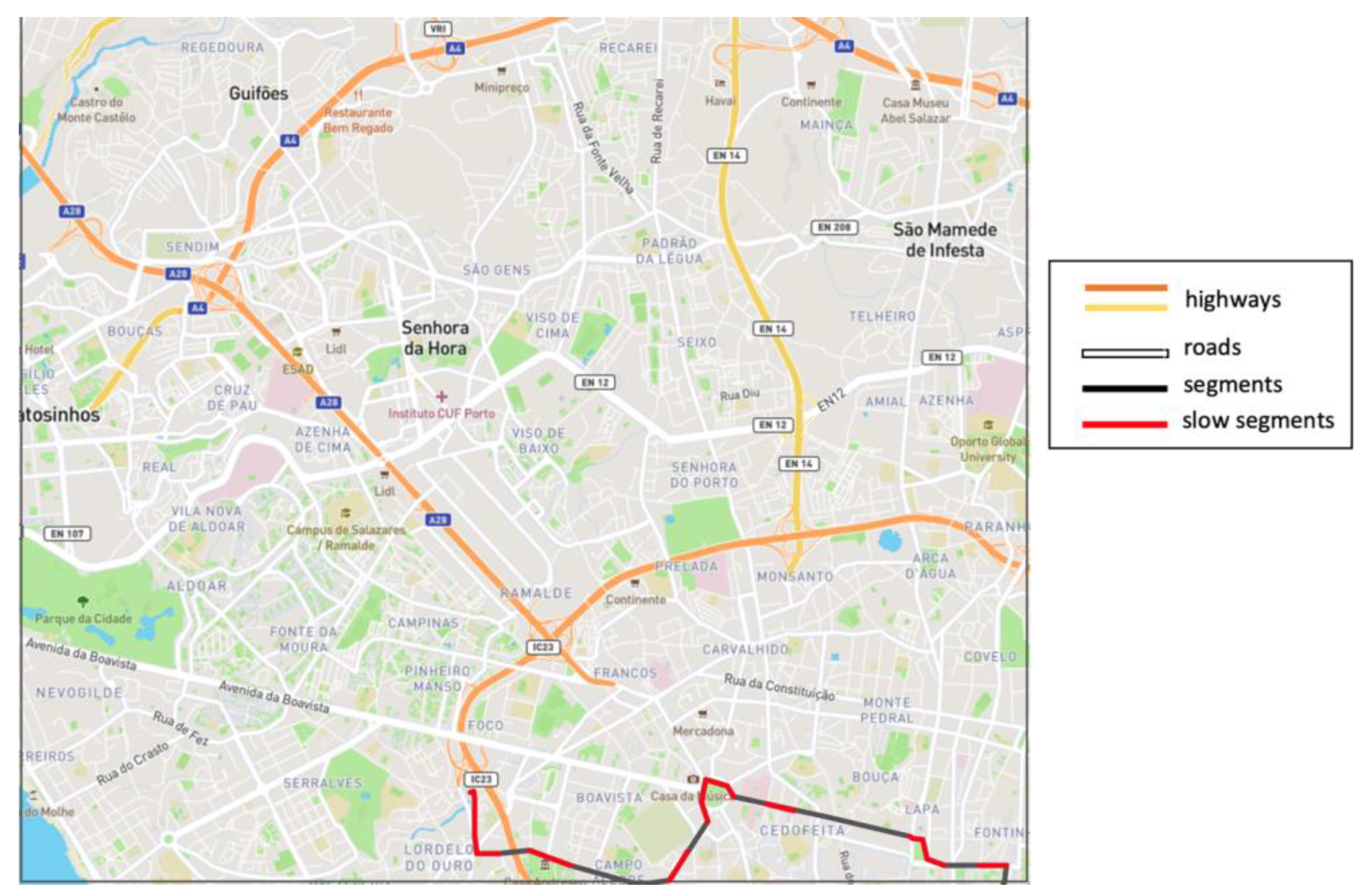
With our proposal, the slow segments of a trajectory can be shown in a spatiotemporal scenario. This feature cannot be obtained with the SPI measure [24]. As a result, we can identify critical points (highest slowness) on the cells, see Figure 18.
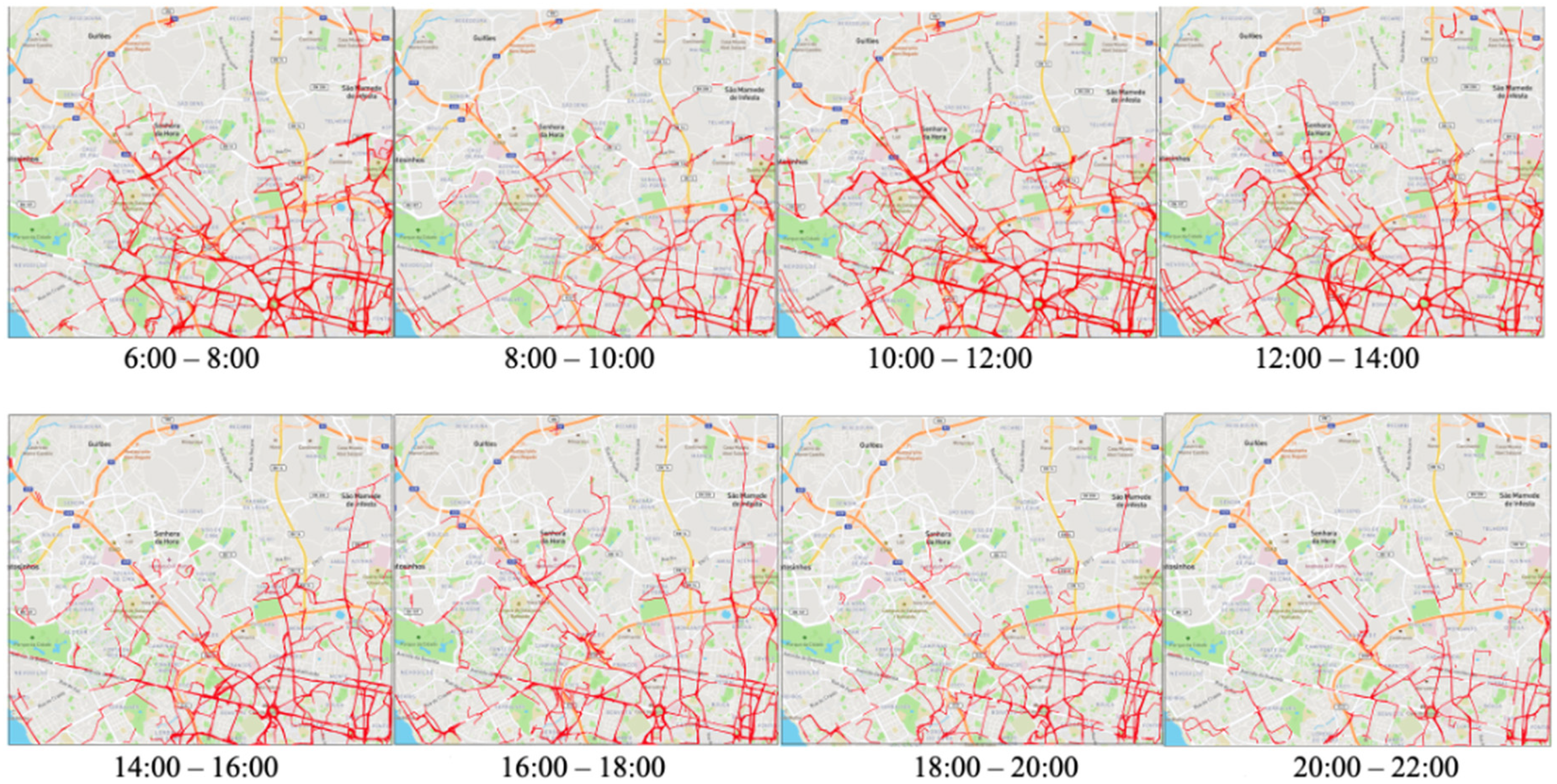
We can also see the slow segment evolution of a cell through the different spatiotemporal scenarios, e.g., see Figure 19; the color conventions are the same as the ones in Figure 18.
From the previous figures, we notice that:
  • From 08:00 to 10:00 on 6 August 2013 there was less slowness in the cell.
  • Around the roundabout, there was more slowness than in the other parts of the cell.
  • Avenida Boavista, Rua de Diogo Bothelio, and Autopista do Norte are main streets that usually have slow segments and critical points in the cell.
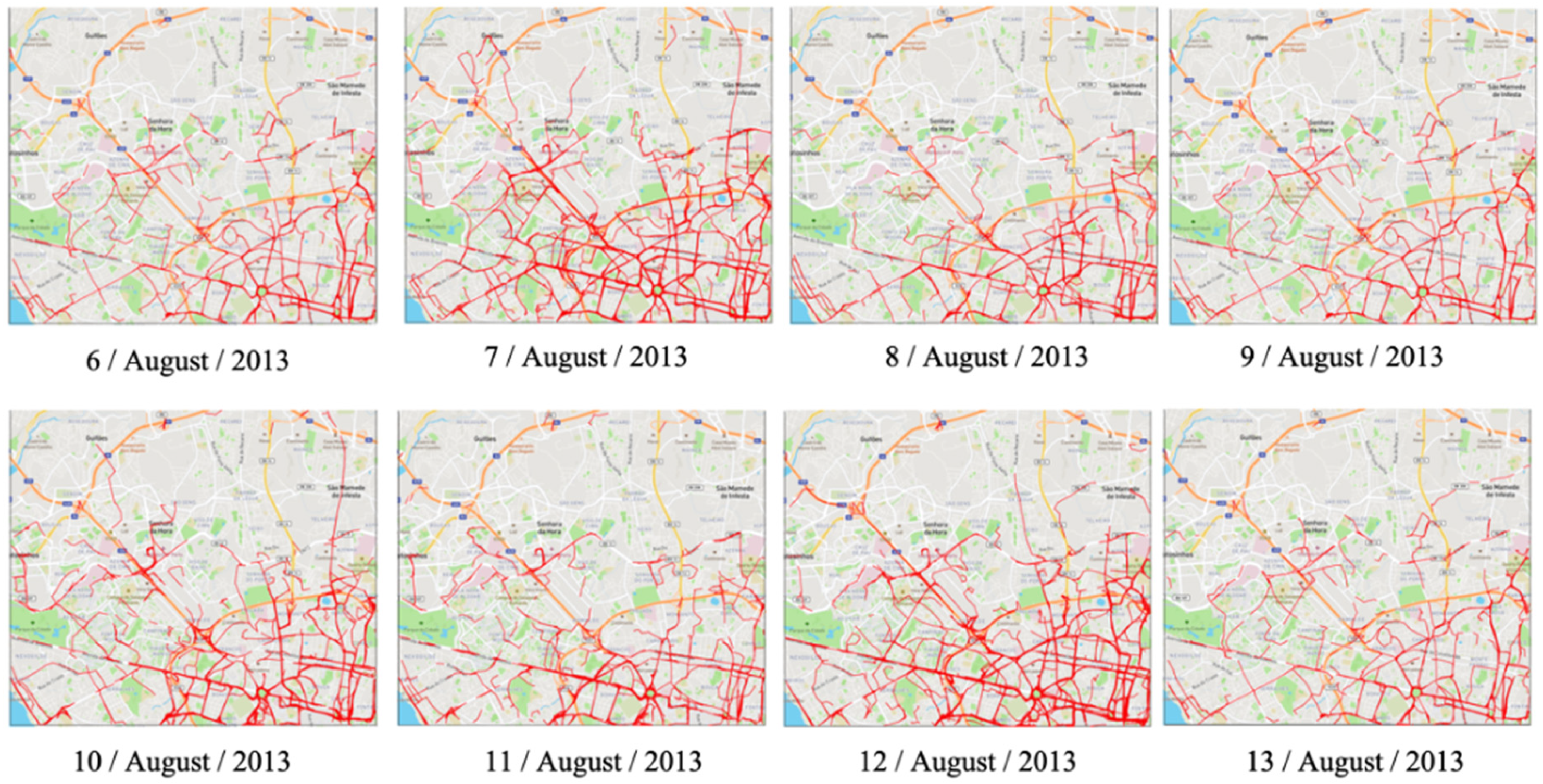
We can also analyze a cell in a spatiotemporal scenario over different days, and see if the critical points (more slowness) are the same in these days, e.g., see Figure 20; the color conventions are the same as the ones in Figure 18.
From the previous figures, we notice that Wednesday (7 August 2013) and Monday (12 August 2013) were the days with more slowness; the other days were similar in slowness.

4. Conclusions

In this paper, we proposed a measure to compute the speed limit rate in each of the cells in which a region is segmented and in a specific temporal segment. The calculation is based on the historical data of trajectories as well as on the identification of slow segments according to a speed limit (MaxSpeed) given by the analyst.
We present and formally define the concepts of speed limit rate and (maximal) slow segments, which are the basic elements to determine the speed limit rate in a cell. Our proposal allows the analyst to segment the region of interest into cells of the desired size (l). Analogously, the time is also segmented. These two segmentations are the basis for developing the notion of a spatiotemporal scenario, a key concept of our proposal.
Our algorithm was tested with historical data (10,485,760 trajectories), and the results stood to reason, e.g., weekdays were slower than weekends, 10 pm to 4 am were the fastest hours (this makes sense because there is usually less traffic during these days and hours, making it easier for vehicles to move faster), and in general, were consistent with the SPI. Although more experiments are needed, our experiments showed the feasibility of our proposal and its potential to identify (sub)regions with high or low-speed limit rates. This could be useful for traffic analysis, including traffic prediction [25]. For example, in our fourth experiment, we showed the evolution of the slow segments of a cell over the course of a day. This evolution can also be obtained for a week or a month and for each temporal segment. In this way, an analyst could detect, according to history, when (temporal segments) and where (roads) slower segments tend to appear in a cell. Another interesting analysis is to see how the slowness of a cell propagates to its adjacent cells in the next temporal segment. Thus, suppose that a driver is currently in cell A and needs to get to cell W. The driver can get to W by following adjacent cells F or L. As a result, if cell F has previously shown, in the next temporal segment, less slowness than cell L, the driver could select this cell because it is faster than cell L.
As future work, we intend to enrich our speed limit rate measure as follows: For example, if only a few vehicles (e.g., less than 5) are passing through a cell and they are moving slowly (e.g., speed ≤ 5 km/h), our speed limit rate measure reports the maximum value (speed limit rate = 1). This is consistent with our definition. However, we could include elements that try to explain why these vehicles are moving slowly, e.g., traffic lights, narrow or bad roads, speed bumps [26], a truck or a set of trucks (a cluster of moving objects) [27] that, e.g., every Monday morning, obstruct a certain road.

Author Contributions

Conceptualization, F.J.M.A. and G.G.; methodology, F.J.M.A., G.G., and S.Z.G.; software, F.J.M.A. and S.Z.G.; validation, F.J.M.A., G.G., and S.Z.G.; formal analysis, F.J.M.A. and G.G.; investigation, F.J.M.A., G.G., and S.Z.G.; resources, F.J.M.A. and S.Z.G.; data curation, F.J.M.A. and S.Z.G.; writing—original draft preparation, F.J.M.A. and G.G.; writing—review and editing, F.J.M.A. and G.G.; visualization, F.J.M.A. and S.Z.G.; supervision, F.J.M.A. All authors have read and agreed to the published version of the manuscript.

Funding

This research received no external funding.

Institutional Review Board Statement

Not applicable.

Informed Consent Statement

Not applicable.

Data Availability Statement

In this study the UCI Machine Learning Repository, the Taxi Service Trajectory-Prediction Challenge, the ECML PKDD 2015 Data Set, and a publicly available dataset that is available at https://archive.ics.uci.edu/mL/datasets/Taxi+Service+Trajectory+-+Prediction+Challenge,+ECML+PKDD+2015 was used (accessed on 10 October 2022).

Conflicts of Interest

The authors declare no conflict of interest.

Appendix A

  • MaxSpeed 30 km/h
Figure A1. Results for the 28 days, cell 6 with MaxSpeed = 30 km/h in the morning.
Informatics 10 00015 g0a1
Figure A2. Results for the 28 days, cell 6 with MaxSpeed = 30 km/h in the afternoon.
Informatics 10 00015 g0a2
Figure A3. Results for the weekends, cell 6 with MaxSpeed = 30 km/h.
Informatics 10 00015 g0a3
Figure A4. Results for the weekdays, cell 6 with MaxSpeed = 30 km/h.
Informatics 10 00015 g0a4
  • MaxSpeed 10 km/h
Figure A5. Results for the 28 days, cell 6 with MaxSpeed = 10 km/h in the morning.
Informatics 10 00015 g0a5
Figure A6. Results for the 28 days, cell 6 with MaxSpeed = 10 km/h in the afternoon.
Informatics 10 00015 g0a6
Figure A7. Results for the weekends, cell 6 with MaxSpeed = 10 km/h.
Informatics 10 00015 g0a7
Figure A8. Results for the weekdays, cell 6 with MaxSpeed = 10 km/h.
Informatics 10 00015 g0a8

References

  1. Ranacher, P.; Tzavella, K. How to Compare Movement? A Review of Physical Movement Similarity Measures in Geographic Information Science and Beyond. Cartogr. Geogr. Inf. Sci. 2014, 41, 286–307. [Google Scholar] [CrossRef] [PubMed] [Green Version]
  2. Magdy, N.; Sakr, M.A.; El-Bahnasy, K. A Generic Trajectory Similarity Operator in Moving Object Databases. Egypt. Inform. J. 2017, 18, 29–37. [Google Scholar] [CrossRef] [Green Version]
  3. Dodge, S.; Weibel, R.; Lautenschütz, A.-K. Towards a Taxonomy of Movement Patterns. Inf. Vis. 2008, 7, 240–252. [Google Scholar] [CrossRef] [Green Version]
  4. Yanagisawa, Y.; Satoh, T. Clustering Multidimensional Trajectories Based on Shape and Velocity. In Proceedings of the 22nd International Conference on Data Engineering Workshops (ICDEW’06), Atlanta, GA, USA, 3–7 April 2006; p. 12. [Google Scholar]
  5. Güting, R.H.; Schneider, M. The Morgan Kaufmann Series in Data Management Systems. In Moving Objects Databases; Elsevier Science: San Francisco, CA, USA, 2005; ISBN 9780080470757. [Google Scholar]
  6. Andrienko, N.; Andrienko, G. Visual Analytics of Movement: An Overview of Methods, Tools and Procedures. Inf. Vis. 2013, 12, 3–24. [Google Scholar] [CrossRef] [Green Version]
  7. Chen, W.; Guo, F.; Wang, F.-Y. A Survey of Traffic Data Visualization. IEEE Trans. Intell. Transp. Syst. 2015, 16, 2970–2984. [Google Scholar] [CrossRef]
  8. Rao, A.M.; Rao, K.R. Measuring Urban Traffic Congestion—A Review. Int. J. Traffic Transp. Eng. 2012, 2, 286–305. [Google Scholar] [CrossRef] [Green Version]
  9. Kohan, M.; Ale, J.M. Discovering Traffic Congestion through Traffic Flow Patterns Generated by Moving Object Trajectories. Comput. Environ. Urban Syst. 2019, 80, 1–14. [Google Scholar] [CrossRef]
  10. Raffaetà, A.; Leonardi, L.; Marketos, G.; Andrienko, G.; Andrienko, N.; Frentzos, E.; Giatrakos, N.; Orlando, S.; Pelekis, N.; Roncato, A.; et al. Visual Mobility Analysis Using T-Warehouse. Int. J. Data Warehous. Min. 2011, 7, 1–23. [Google Scholar] [CrossRef] [Green Version]
  11. Alsahfi, T.; Almotairi, M.; Elmasri, R. A Survey on Trajectory Data Warehouse. Spat. Inf. Res. 2020, 28, 53–66. [Google Scholar] [CrossRef] [Green Version]
  12. Malinowski, E.; Zimányi, E. Advanced Data Warehouse Design; Springer: Berlin/Heidelberg, Germany, 2008. [Google Scholar]
  13. Leonardi, L.; Orlando, S.; Raffaetà, A.; Roncato, A.; Silvestri, C.; Andrienko, G.; Andrienko, N. A General Framework for Trajectory Data Warehousing and Visual OLAP. GeoInformatica 2014, 18, 273–312. [Google Scholar] [CrossRef]
  14. Beliakov, G.; Gagolewski, M.; James, S.; Pace, S.; Pastorello, N.; Thilliez, E.; Vasa, R. Measuring Traffic Congestion: An Approach Based on Learning Weighted Inequality, Spread and Aggregation Indices from Comparison Data. Appl. Soft Comput. 2018, 67, 910–919. [Google Scholar] [CrossRef]
  15. de Almeida, D.; de Souza Baptista, C.; de Andrade, F.; Soares, A. A Survey on Big Data for Trajectory Analytics. ISPRS Int. J. Geo-Inf. 2020, 9, 88. [Google Scholar] [CrossRef] [Green Version]
  16. Wang, S.; Bao, Z.; Culpepper, J.S.; Cong, G. A Survey on Trajectory Data Management, Analytics, and Learning. ACM Comput. Surv. 2021, 54, 1–36. [Google Scholar] [CrossRef]
  17. U.S. Department of Transportation, Federal Highway Administration. Traffic Analysis Tools Program. Available online: https://ops.fhwa.dot.gov/trafficanalysistools/type_tools.htm (accessed on 6 January 2023).
  18. Traffic Micro-simulation model. Multicriteria Planning (Mcrit Ltd). Available online: https://mcrit.com/services/systems-and-software-development/traffic-micro-simulation-models (accessed on 6 January 2023).
  19. Afrin, T.; Yodo, N. A Survey of Road Traffic Congestion Measures towards a Sustainable and Resilient Transportation System. Sustainability 2020, 12, 4660. [Google Scholar] [CrossRef]
  20. Yuan, H.; Li, G. A Survey of Traffic Prediction: From Spatio-Temporal Data to Intelligent Transportation. Data Sci. Eng. 2021, 6, 63–85. [Google Scholar] [CrossRef]
  21. Di Felice, P.; Clementini, E. Topological Relationships. In Encyclopedia of Database Systems; Liu, L., Özsu, M.T., Eds.; Springer: Boston, MA, USA, 2009; pp. 3140–3143. ISBN 978-0-387-39940-9. [Google Scholar]
  22. Allen, J.F. Maintaining Knowledge about Temporal Intervals. Commun. ACM 1983, 26, 832–843. [Google Scholar] [CrossRef] [Green Version]
  23. Dua, D.; Graff, C. UCI Machine Learning Repository; School of Information and Computer Science, University of California: Irvine, CA, USA, 2019; Available online: https://archive.ics.uci.edu/ml/datasets/Taxi+Service+Trajectory+-+Prediction+Challenge,+ECML+PKDD+2015 (accessed on 10 October 2022).
  24. He, F.; Yan, X.; Liu, Y.; Ma, L. A Traffic Congestion Assessment Method for Urban Road Networks Based on Speed Performance Index. Procedia Eng. 2016, 137, 425–433. [Google Scholar] [CrossRef] [Green Version]
  25. Vlahogianni, E.I.; Karlaftis, M.G.; Golias, J.C. Short-Term Traffic Forecasting: Where We are and Where We’re Going. Transp. Res. Part C Emerg. Technol. 2014, 43, 3–19. [Google Scholar] [CrossRef]
  26. Salau, T.A.O.; Adeyefa, A.O.; Oke, S.A. Vehicle Speed Control Using Road Bumps. Transport 2004, 19, 130–136. [Google Scholar] [CrossRef] [Green Version]
  27. Ossama, O.; Mokhtar, H.M.O.; El-Sharkawi, M.E. An Extended K-Means Technique for Clustering Moving Objects. Egypt. Inform. J. 2011, 12, 45–51. [Google Scholar] [CrossRef]
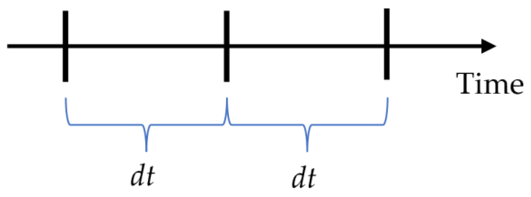
Figure 1. Temporal segmentation.
Informatics 10 00015 g001
Figure 2. Spatial segmentation: region of interest segmented into cells (array of order 3 × 4).
Informatics 10 00015 g002
Figure 3. Segment of a trajectory T in a cell of a spatiotemporal scenario.
Informatics 10 00015 g003
Figure 4. Maximal segment of a trajectory T in a cell of a spatiotemporal scenario.
Informatics 10 00015 g004
Figure 5. Trajectory with two maximal slow segments in a cell of a spatiotemporal scenario.
Informatics 10 00015 g005
Figure 6. A cell with three trajectories.
Informatics 10 00015 g006
Figure 7. Example of a trajectory taken from the dataset.
Informatics 10 00015 g007
Figure 8. Porto segmented into sixteen cells of the grid.
Informatics 10 00015 g008
Figure 9. Cell 6.
Figure 9. Cell 6.
Informatics 10 00015 g009
Figure 10. Calculated speed limit rates for the 28 days, cell 6 with MaxSpeed = 50 km/h in the morning.
Informatics 10 00015 g010
Figure 11. Calculated speed limit rates for the 28 days, cell 6 with MaxSpeed = 50 km/h in the afternoon.
Informatics 10 00015 g011
Figure 12. Calculated speed limit rates for the weekends, cell 6 with MaxSpeed = 50 km/h.
Informatics 10 00015 g012
Figure 13. Calculated speed limit rates for the weekdays, cell 6 with MaxSpeed = 50 km/h.
Informatics 10 00015 g013
Figure 14. Calculated SPI for the entire month, cell 6 with Vmax = 100 km/h in the morning.
Informatics 10 00015 g014
Figure 15. Calculated SPI for the entire month, cell 6 with Vmax = 100 km/h in the afternoon.
Informatics 10 00015 g015
Figure 16. Calculated SPI for the weekends, cell 6 with Vmax = 100 km/h.
Informatics 10 00015 g016
Figure 17. Calculated SPI for the weekdays, cell 6 with Vmax = 100 km/h.
Informatics 10 00015 g017
Figure 18. Slow segments (in red) of a trajectory with Maxspeed = 60 km/h, 6 August 2013 8:00:00–10:00:00.
Informatics 10 00015 g018
Figure 19. Slow segment evolution of a cell through different spatiotemporal scenarios on Tuesday 6 August 2013, 60 km/h.
Informatics 10 00015 g019
Figure 20. Slow segment evolution of a cell from 6 August 2013 to 13 August 2013 and from 8:00–10:00, 60 km/h.
Informatics 10 00015 g020
Table 1. Summary of segment types in a cell (R[v, w]).
                                                                             Conditions
(a) guarantees the spatial inclusion of all the CPs of a segment in the cell R[v, w].
(b) guarantees the temporal inclusion of all the CPs of a segment in the temporal segment associated with the cell R[v, w].
(c) and (d) guarantee that the segment is the one with the maximum size with respect to conditions (a) and (b).
(e) guarantees that the speed among all the consecutive CPs of a segment is less than MaxSpeed.
(f) and (g) guarantee that the segment has the maximum number of CPs with respect to conditions (a), (b), and (e).
Segment TypeConditions
Segment(a) and (b)
Maximal segment(a), (b), (c), and (d)
Slow segment(a), (b), and (e)
Maximal slow segment(a), (b), (e), (f), and (g)
Note that a slow segment may, in turn, be a maximal segment; it occurs when it also meets conditions (c) and (d) or equivalently when a maximal segment also meets conditions (e), (f), and (g).
Table 2. Calculated speed limit rates for 3 August 2013 with MaxSpeed = 50 km/h.
TempSegCell
12345678910111213141516
(00:00, 02:00]ND0.471NDND0.0890.2680.606ND0.1530.3310.438NDND0.485NDND
(02:00, 04:00]0.0480.405NDND0.1570.3310.569NDND0.4230.569NDNDNDND0.601
(04:00, 06:00]0.5390.514NDND0.0690.4050.650NDND0.4210.5340.247NDNDNDND
(06:00, 08:00ND0.568NDND0.0910.3740.5860.2640.5710.4380.627NDND0.622NDND
(08:00, 10:00]0.4090.782NDND0.0830.3960.659ND0.3990.4240.4740.3450.1070.3201ND
(10:00, 12:00]0.1760.587NDND0.0940.3810.7340.4080.44010.4520.5281ND10.3520.090
(12:00, 14:00]0.0640.660NDND0.0680.4040.6910.507ND0.5000.505NDNDNDNDND
(14:00, 16:00]0.5140.627NDND0.8280.4360.727NDND0.4580.494NDND10.587ND
(16:00, 18:00]ND0.570NDND0.1690.4550.738ND0.8890.4550.504NDND1NDND
(18:00, 20:00]ND0.594NDND0.0850.4140.6190.0550.4560.3980.458ND0.5370.220NDND
(20:00, 22:00]00.274NDND0.1010.3640.6460.2060.5000.3620.4190.504ND0.3130.435ND
(22:00, 00:00]00.449NDND0.1120.2710.5980.1380.2770.3200.3740.257ND0.5280.413ND
Table 3. Calculated speed limit rates for 3 August 2013 with MaxSpeed = 40 km/h.
TempSegCell
12345678910111213141516
(00:00, 02:00]ND0.327NDND0.0560.1730.433ND0.0390.2110.275NDND0.485NDND
(02:00, 04:00]0.0250.257NDND0.1000.2180.439NDND0.2760.392NDNDNDND0.441
(04:00, 06:00]0.2400.371NDND0.0530.2800.496NDND0.2770.3830.189NDNDNDND
(06:00, 08:00ND0.358NDND0.0680.2500.458ND0.4480.2900.442NDND0.062NDND
(08:00, 10:00]0.2500.494NDND0.0510.2660.501ND0.2360.2600.2980.2740.00.1280.769ND
(10:00, 12:00]0.1550.379NDND0.0800.2560.572ND0.2720.2920.3250.776ND0.0250.1020.090
(12:00, 14:00]0.0420.507NDND0.0470.2750.523NDND0.3300.319NDNDNDNDND
(14:00, 16:00]0.2260.426NDND0.4340.2930.553NDND0.2760.329NDND0.3590.237ND
(16:00, 18:00]ND0.418NDND0.1170.2950.567ND0.5600.2730.308NDND1.000NDND
(18:00, 20:00]ND0.320NDND0.0380.2710.456ND0.4110.2310.272ND0.2750.102NDND
(20:00, 22:00]00.234NDND0.0590.2310.494ND0.3000.2180.2470.261ND0.1510.435ND
(22:00, 00:00]00.251NDND0.0760.1720.439ND0.1090.2020.2260.202ND0.3770.206ND
Table 4. Average calculated speed limit rate by day and TempSeg of all the cells, MaxSpeed = 50 km/h (weekends in green).
DateTempSeg
(00:00, 02:00](02:00, 04:00](04:00, 06:00](06:00, 08:00](08:00, 10:00](10:00, 12:00](12:00, 14:00](14:00, 16:00](16:00, 18:00](18:00, 20:00](20:00, 22:00](22:00, 00:00]
3 August 20130.4110.4730.5030.5070.4890.5240.5250.5290.5380.4730.4480.391
4 August 20130.3940.4050.4630.4490.4370.4790.5160.4690.4730.4390.3700.280
5 August 20130.3740.5440.5390.4920.5200.5400.5410.4950.4860.4200.3960.318
6 August 20130.3800.5250.5490.5150.5780.5510.5520.5000.4920.4980.4120.351
7 August 20130.4080.5380.5310.4900.5650.5650.5800.5110.4870.4620.3940.374
8 August 20130.4400.5250.5240.4730.5880.5740.5680.5100.4630.4480.4290.363
9 August 20130.4260.5350.5570.4660.5650.5370.5470.5350.5520.4740.4380.396
10 August 20130.4120.4830.4950.4490.4570.5090.5020.5000.5340.4820.4470.412
11 August 20130.4110.4110.4580.3850.4510.4680.4810.5120.4750.4140.3810.315
12 August 20130.4120.5130.5370.4850.5560.5650.5600.4870.4780.4580.4000.351
13 August 20130.4090.5080.5270.4710.5400.5640.5450.4900.5050.4940.4490.352
14 August 20130.3700.5300.5360.4850.5430.5760.5680.4790.5280.4660.4480.384
15 August 20130.3840.4190.4670.4170.4670.4640.5100.5070.4900.4730.3930.363
16 August 20130.4070.4960.5420.4710.5440.5290.5520.4840.5190.4970.4320.404
17 August 20130.3860.4710.5080.4270.5000.5610.5430.4970.5300.4740.4290.374
18 August 20130.3910.4170.4290.4120.4930.4750.5050.4610.4810.4210.4230.317
19 August 20130.3910.5290.5550.4940.5350.5500.5480.5170.5240.4420.3940.337
20 August 20130.3810.4940.5220.4720.5460.5590.5600.4930.5320.4680.3990.354
21 August 20130.3740.4870.5220.4770.5330.5280.5690.5080.4930.4710.4240.354
22 August 20130.3790.4800.5210.5090.5610.5680.5450.5270.5020.4340.3420.391
23 August 20130.4180.5210.5330.4850.5480.5500.5630.5170.5120.4670.4100.395
24 August 20130.3780.4630.5120.4610.4950.5480.5800.5280.5340.4880.4330.392
25 August 20130.3630.4110.4860.4330.4790.5180.5220.4590.5280.4260.3620.324
26 August 20130.3850.5060.5080.4900.5830.5690.5560.4850.5190.4230.3800.322
27 August 20130.3820.5220.5140.4850.5720.5450.5550.5130.5240.4310.3500.340
28 August 20130.3880.5030.5330.5200.5540.5520.5430.5300.5190.4300.4360.366
29 August 20130.4080.4920.5170.4980.5960.5760.5390.5020.5090.4590.4200.354
20 August 20130.3820.5430.5300.4700.5320.5620.5650.5010.5300.4920.4310.372
Disclaimer/Publisher’s Note: The statements, opinions and data contained in all publications are solely those of the individual author(s) and contributor(s) and not of MDPI and/or the editor(s). MDPI and/or the editor(s) disclaim responsibility for any injury to people or property resulting from any ideas, methods, instructions or products referred to in the content.