1. Introduction
In mathematical finance, principal component analysis (PCA) is used to reduce dimensionality in the explanation of a vector of asset returns; see, for instance,
Alexander (
2001) for discrete-time model applications. The methodology has also been used in continuous-time stochastic processes for financial applications; see
Escobar et al. (
2010) and
Escobar and Olivares (
2013) for its usage in collateralized debt obligations (CDO) and exotic financial derivatives pricing, as well as
Escobar and Gschnaidtner (
2018) and more generally
De Col et al. (
2013) for factor and PC analyses applications to foreign exchange data.
When modeling financial or any complex data, one can focus on capturing the stylized facts reported in the literature. The best-known features of financial data are as follows: fat tails, changing volatilities and correlations, the leverage effect and co-volatility movements. Examples of a refined fact of financial data are the smiles and smirks of the implied volatility surface. To capture them, in
Christoffersen et al. (
2009), the authors proposed a PCA-inspired stochastic covariance (SC) model using the popular Heston stochastic volatility model
Heston (
1993) as the underlying component.
These features can be captured by rich SC models, with proper marginal structures. SC models have received significant attention in the literature; the best-known representatives are the stochastic Wishart family, see
Da Fonseca et al. (
2007);
Gouriéroux (
2006), and the Ornstein–Uhlenbeck (OU) family, see
Muhle-Karbe et al. (
2012), of models, as well as general linear-quadratic jump-diffusions, see
Cheng and Scaillet (
2007). Even though these models show realistic advantages over the classical Black–Scholes model, they lose their tractability as a result of an increase in model dimensions (i.e., an increase in the number of parameters and simulation paths). This is commonly known as the curse of dimensionality, and PCA is a viable method to control the problem with dimensionality. Inspired by this, principal component stochastic volatility (PCSV) models are built from a linear combination of tractable one-dimensional counterparts. Their applications have been studied in a series of papers since 2010; see, for example,
De Col et al. (
2013);
Escobar (
2018);
Escobar et al. (
2010);
Escobar-Anel and Moreno-Franco (
2019).
Current PCSV models rely on Heston SV for the components, also known as the 1/2 model. A new model for single assets, namely, the 4/2 volatility process, was masterfully presented in
Grasselli (
2016). Notably, the Heston model (the 1/2 model) predicts that the implied volatility skew will flatten when the instantaneous volatility increases (e.g., financial crises), while another embedded structure, the 3/2 model see
Platen (
1997) predicts steeper skews. The author argues that the two processes complement each other in better explaining the implied volatility surface. There are many interesting, recent generalizations of the 4/2 model, see, for example,
Cui et al. (
2021) and
Kirkby and Nguyen (
2020) and the literature therein.
The works presented above mostly target the equity market and are built based on geometric Brownian motion (GBM)-type processes, and they are hence not suitable for commodities and volatility indexes. These asset classes display mean-reverting and spillover effects, both of which are stylized facts not seen in equities. Mean-reverting effects capture the stationary behavior of prices, which tend to go back to a long-term mean. On the other hand, spillover refers to the impact of one asset on the trends (drift) of other assets (i.e., the impact of one asset on the long term average “stationary price” of a second asset). Our modeling in this paper will ensure that these two facts are captured.
Our modeling is inspired by a recent paper by
Cheng et al. (
2019) that introduces a generalized multivariate mean-reverting 4/2 factor analysis (FA) model. The model uses the one-dimensional mean-reverting 4/2 stochastic volatility proposed by
Escobar-Anel and Gong (
2020) as the underlying model. They obtained an analytical representation of the characteristic function (c.f.) of a vector of asset prices as well as a second conditional c.f. for non-mean-reverting nested cases. Thus, the FFT-based option pricing method, for example
Carr and Madan (
1999), can be used, and exact simulation is possible. The authors further identified a set of conditions that not only produces well-defined changes of measure, but also avoids local martingales for risk-neutral pricing purposes.
In this paper, we make several contributions to the literature:
We studied in detail a multivariate mean-reverting 4/2 stochastic volatility model based on PCA, which is inspired in the general framework of
Cheng et al. (
2019). The SC in the new model is decomposed into constant eigenvectors that capture the correlation among assets and a diagonal eigenvector matrix whose entries are modeled by the 4/2 process.
The PCA structure allows us to find a semi-closed-form c.f. for the vector of returns. It permits the extension to multidimensions of simple but accurate approximation approaches, first introduced in
Escobar-Anel and Gong (
2020) for one dimension, to find closed-form approximations to the c.f., which are proven to be accurate for realistic parameter settings.
We use the estimation approaches developed in
Escobar-Anel and Gong (
2020) to estimate the parameters for special cases of the proposed model. Here, we use two pairs of bivariate time series capturing both the asset and its variance. Estimation of multidimensional processes is rare in the literature, and our work demonstrates that many, but not all, of the parameters are statistically significant, confirming stylized facts of commodity prices and volatility indexes such as stochastic correlation and spill-over effects.
A risk management application, based on a constant proportion strategies portfolio, for example
Merton (
1975) and
DeMiguel et al. (
2009), demonstrates the accuracy of the approximation.
The rest of the paper is organized as follows: in
Section 2, we define the model and derive two sub-models for two parametric constructions. Then, in
Section 3, we expand the theoretical results for the c.f.s obtained in
Cheng et al. (
2019) with approximations. In
Section 4, we focus on estimation for the multivariate mean-reverting 4/2 stochastic volatility model. The estimation method considered is based on the method developed in
Escobar-Anel and Gong (
2020) with the introduction of a new scaling factor. Thereafter, in
Section 5, we construct a portfolio with two risky assets and one risk-free cash account, and we subsequently calculate the value-at-risk (VaR) at a 95% level using various techniques. Finally,
Section 6 concludes the paper.
2. Model Definition
In this section, we define the general model. We first introduce a model with spillover effects, and we later cover models with separable spillover effects and no spillover effects as special cases. We also study the implications of the model on the covariance process.
2.1. General Model Setup
Suppose
is a vector of assets. The dynamics for each asset
under the so-called historical measure
is defined as
where
and
are independent Brownian motions if
, and they are correlated if
, that is, the quadratic variation
, where
is constant. The parameters for each
process are positive and satisfy the Feller condition:
. Moreover, we assume that the mean-reverting level of
decreases as
j increases; that is,
, for
. This last feature is intended to sort the eigenvalues in order of importance, and
’s measure the “weight” of the 3/2 components.
This model is unlike a traditional mean-reverting model, as it takes into account the spillover effects in the drift, which appear in the form of
. We mentioned above that the spillover effects show the impacts of one asset on others; these impacts shall not be confused with correlations. The correlations are reflected in the price trend of both assets, capturing co-movements between assets. Spillover effects describe the impact on the mean-reverting level of one asset by others (i.e., the shift in the long term mean due to the movements of other assets). The concept of spillover effects can be understood as how much, for example, a demand curve of one good shifts according to the change in factors of other goods. In addition, although this paper does not dwell into risk-neutral pricing, we should highlight that changes of measure are feasible on each principal component along the lines of Proposition 4 in
Escobar-Anel and Gong (
2020), this is changes of the type:
,
.
Equation (
1) can be written in matrix form as follows:
where
is a vector of independent standard Brownian motions;
and
.
We first assume that the eigenvalues of the matrix
are all negative; this is similar to the literature, see
Langetieg (
1980) and
Larsen (
2010). This assumption will be used to explain some of the estimation results. Here,
captures the spillover effects, while
contains risk premiums associated with the assets, and the long-term average for the assets is determined by
.
We next assume a principal component decomposition on the instantaneous covariance matrix
:
, where
is an orthogonal matrix with constant entries, and it captures the correlations among assets. We craft the matrix
in such a way that allows for c.f. analytical approximations; that is
, where
and
denotes the Hadamard product of
. The dynamics of log price
is as follows:
Based on the applications, our model can be reduced to three subcases for which we are able to approximate the c.f. with analytic functions:
: This is a generalization of
Escobar et al. (
2010) to multivariate mean-reverting asset classes. If
, we get the model considered in
Benth (
2011).
: This case applies to the assets whose price series demonstrates an abnormal increase or decrease, but no leverage effect is observed for the assets of interest. The term “leverage effect" was first defined and studied in
Black (
1976). It describes the negative correlation between an asset’s volatility and its return.
: This case can be generated by either of the two previous cases. It applies better to assets that exhibit mild behavior in their price series; at the same time, no leverage effect is identified.
We explain how to approximate the c.f. with analytic functions for these three cases in
Section 3.
2.1.1. Separable Spillover Effect
In this section, we assume a convenient structure in the spillover matrix
to obtain the c.f., and by doing so, we obtain another solvable case. Here, we further simplify the model by rewriting it in terms of
n independent processes. We demonstrate this procedure by first writing Equation (
3) in matrix form:
Multiplying both sides of Equation (
4) by
, we get
Suppose the matrix
can be written as follows:
, where
is a diagonal matrix (i.e., whose entries are eigenvalues of
). Using this result, and applying a simple transformation
, we arrive at a new mean-reverting process with diagonal matrix
:
Each element of
is a mean-reverting 4/2 stochastic volatility process, as in
Escobar-Anel and Gong (
2020). That is,
where
, and
are the entries of
. Furthermore,
is also a vector of independent processes.
2.1.2. Model with No Spillover Effects
In this section, we assume no spillover effects among the assets (i.e., matrix
is diagonal). This further simplifies our model to
The corresponding matrix representation has the same form:
with
. The dynamics of log price
are then
2.2. Properties of the Variance Vector
We devote this subsection to exploring the properties of the variance vector. This is important for understanding the instantaneous volatilities implied by our model. Recall that empirical data is related to these volatilities; therefore, one should ensure that these implied processes reflect the stylized facts of the data they cater to.
Let
denote the variance vector; by definition, this is
. As defined before,
is a vector of 4/2 processes (the sum of 1/2 and 3/2 processes). Therefore,
can be written in terms of a linear combination of these two processes:
This model for the variance can be interpreted as factor model with n 4/2 factors. Due to the popularity of factor models for explaining asset classes, it stands to reason that volatility indexes (these variances) can also be expressed in terms of factors, which could reflect intrinsic and systemic economical movements.
One can obtain the dynamics of
more explicitly:
From the above stochastic differential Equation (SDE), we are able to obtain the variance and covariance of the vector
via quadratic variations. Note that these can be interpreted as the volatility of variance and the correlation among variances (co-volatility movement), respectively:
Equations (
10) and (
11) suggest that the instantaneous variance and covariance of
are locally stochastic (i.e., driven by the same Brownian as the underlying).
3. Characteristic Functions and Approximations
In this section, we derive the c.f.s for the previously presented cases involving spillover effects and no spillover effects, using Proposition 2 and Corollary 1 from
Cheng et al. (
2019), in line with the approximation approach from
Escobar-Anel and Gong (
2020). In
Escobar-Anel and Gong (
2020), the authors obtained analytical approximations of the c.f.’s for the special cases
;
using results from
Grasselli (
2016). Taking advantage of the principal component structure of the model, we demonstrate that the c.f. representations boil down to a multiplication of one-dimensional approximations.
Next, we show the c.f. for the general model and its submodels described in
Section 2, namely the model with general spillover effects (
Section 3.1) and the model with separable spillover effects (
Section 3.2). Then, in
Section 3.3, we present the principle used to approximate the c.f.’s.
3.1. Characteristic Function for Model with Spillover Effects
Let us first define
such that
is a matrix exponential; then
is represented as
For convenience, we use as the -th component of the matrix . Note that is no longer a mean-reverting process, although it accounts for time-dependent coefficients.
Corollary 1. Let evolve according to the model in Equation (
12).
The c.f. is then given as follows:where , , and . Moreover, is a one-dimensional generalization of the c.f. from Grasselli (2016) provided in Lemma A1 of Cheng et al. (2019). The proof follows as a direct application of the proof of Proposition 2 in
Cheng et al. (
2019).
3.2. Characteristic Function for Model with Separable Spillover Effects
To derive the c.f. of
, we perform the transformation
, recognizing that the c.f. of
has been derived in
Escobar-Anel and Gong (
2020). Hence, the c.f. of
is a product of the corresponding c.f. of
. The result is summarized in the following corollary.
Corollary 2. Let denote the characteristic function provided in Proposition 2.1 in Escobar-Anel and Gong (2020); then, the characteristic function of is given by the following equation:where is a new vector of real numbers with element . The proof is straightforward; using the relationship
, we know that each individual process
is a linear combination of
, and therefore
, processes. The product
can be further written in terms of
:
The independence property of random variables leads to Equation (
13).
3.3. Approximation Principle and Results
We have learned that the c.f. can be written in terms of a product of the c.f.’s of
n independent one-dimensional processes thanks to principal component decomposition. These one-dimensional processes are only different in the structure of the matrix exponential term (i.e.,
), which is deterministic, and they resemble the same
process seen in
Escobar-Anel and Gong (
2020). Therefore, the principles to approximate
follow those adopted in
Escobar-Anel and Gong (
2020). In other words, we only need to calculate an approximation to the individual c.f.
, and the approximation can be realized under three scenarios, as described in
Section 2:
;
and the trivial case of
.
cannot be solved in closed-form due to the lack of a representation of the moment generating function of an integrated Cox-Ingersoll-Ross (CIR) process with time-dependent integrands. Therefore, we propose an analytic function that approximates the unsolvable conditional expectation:
for some complex constants
m and
n:
,
, and
, for
. We propose the following two approximations:
Midpoint:, .
Average:, .
The approximated conditional expectation is solvable, as it fits the framework of
Grasselli (
2016). We summarize the results in the following corollary for the general model with spillover effects, which includes separable spillover effects as a special case.
Corollary 3. Given deterministic functions and , defined in Lemma A1 in Cheng et al. (2019), and , defined in Corollary 1 for ,can be approximated by analytic functions for constants and satisfyingunder three scenarios: : Given , and , . If , then : Given and , . If , , then
Corollary 3 follows directly from Propositions 2.2 and 2.3 in
Escobar-Anel and Gong (
2020). The approximation for the c.f. when there are no spillover effects follows the same procedure as presented in Corollary 3. For the case when the spillover effects are separable, we obtain a sum of independent mean-reverting 4/2 stochastic volatility processes, as indicated in Equation (
6). As a result, Propositions 2.2 and 2.3 in
Escobar-Anel and Gong (
2020) can be directly applied to approximate the c.f.s for these processes.
4. Estimation
In this section, we consider the model with separable spillover effects as the underlying model for estimation. In this way, on the one hand, we fulfill the purpose of studying spillover effects among assets, and on the other hand, we avoid the complexity of a matrix exponential
1. Recall that the model with separable spillover effects can be expressed as follows:
where
is constructed such that it can be decomposed into a product of three matrices:
. In this case,
is a linear combination of independent processes
, that is,
with
For simplicity, we focus on two dimensions, hence studying pairs of assets with their respective volatility indexes. For example, VIX (VVIX) and VSTOXX (VVSTOXX), USO (OVX) and GLD (GVZ), or USO (OVX) and SLV (VXSLV). Then, we follow the same estimation procedure outlined in
Escobar-Anel and Gong (
2020), splitting the parameters into two groups: volatility group and drift group.
After a data description in
Section 4.1,
Section 4.2 estimates tEstVolGpnder the model with separable spillover effects, we first need to estimate covariance matrix (
) from asset data as a long-term average of the SC matrix (
). This permits us to produce and estimate for the constant eigenvectors, denoted as
. With the estimated eigenvectors, we decompose our original asset processes into the sum of independent mean-reverting 4/2 models. The volatility group then consists of parameters for the underlying CIR processes driving the principal components:
.
Section 4.3 tackles the estimation of drift group parameters, using least squares.
Volatility indexes are functions of implied volatility, model free and directly calculated from option prices from the market. Here, we use volatility indexes data as a convenient proxy for instantaneous volatility. In fact, instantaneous volatility is rather impossible to capture from empirical data, even with high-frequency data, as it requires instantaneous periods rather than the available discrete periods. On the other hand, once a model is specified, volatility indexes can be used to represent instantaneous volatility with some multiplicative (scaling) adjustment or factor; see, for example
Luo and Zhang (
2012),
Zhang and Zhu (
2006) and references therein. The relationship between the instantaneous volatility and the volatility index, for example VIX, can be expressed in terms of a closed-form equation, where the difference between the two lies in a multiplicative factor. In a recent paper, see
Lin et al. (
2017), the author determines the connection between instantaneous and implied volatility, assuming Grasselli’s 4/2 model
Grasselli (
2016) with jumps.
Due to the short horizon of volatility indexes (21-day options), the multiplicative factor could be close to one in a region of the parametric space, which implies that volatility indexes are almost equal to instantaneous volatilities regardless of the structural choice of the underlying model. As precautions and inspired by these pioneering works, we introduce scale parameters to adjust empirical volatility indexes data to estimate instantaneous volatilities. This is done such that the empirical means of the observed variance series () match the corresponding long-term asset variances. These new scaling parameters are estimated at an early stage and are methodologically independent of other parameters.
4.1. Data Description
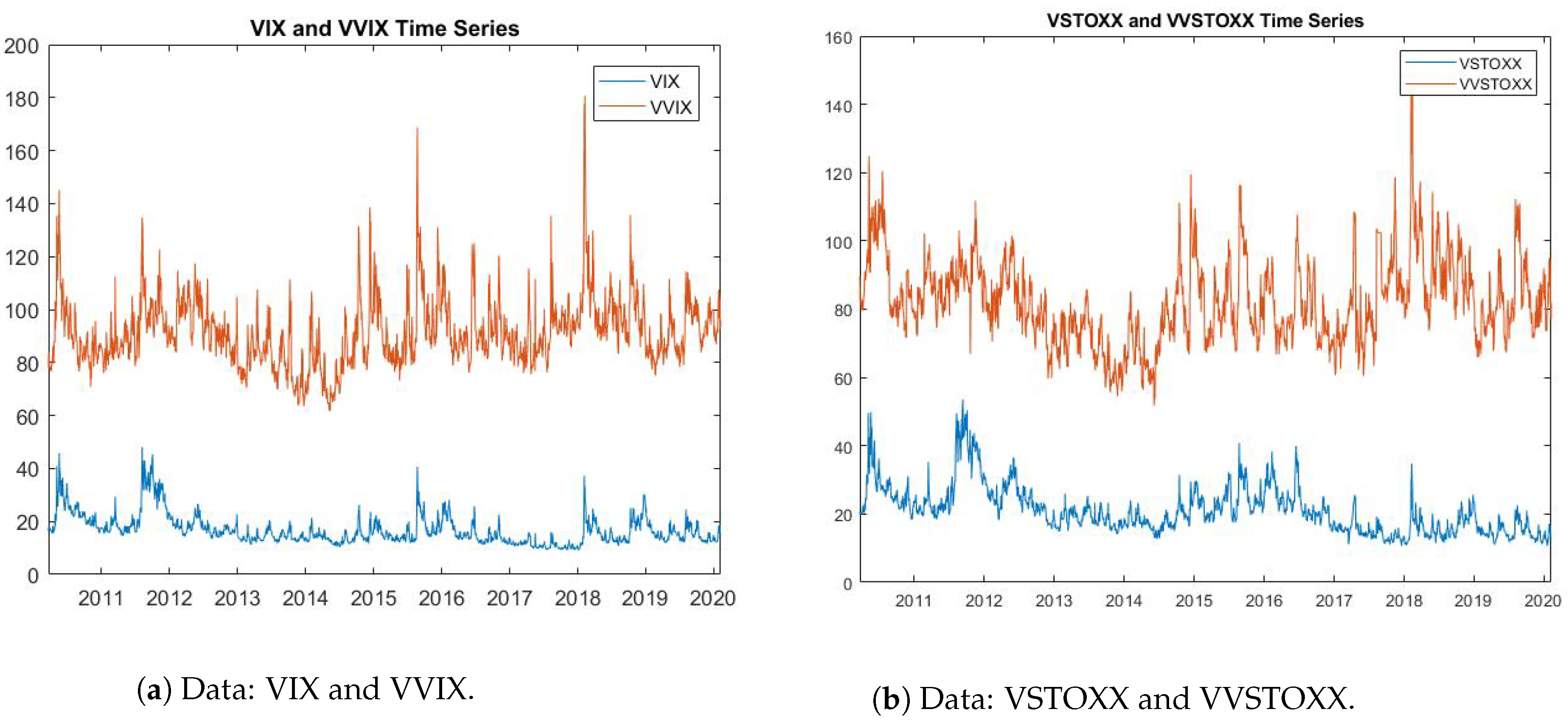
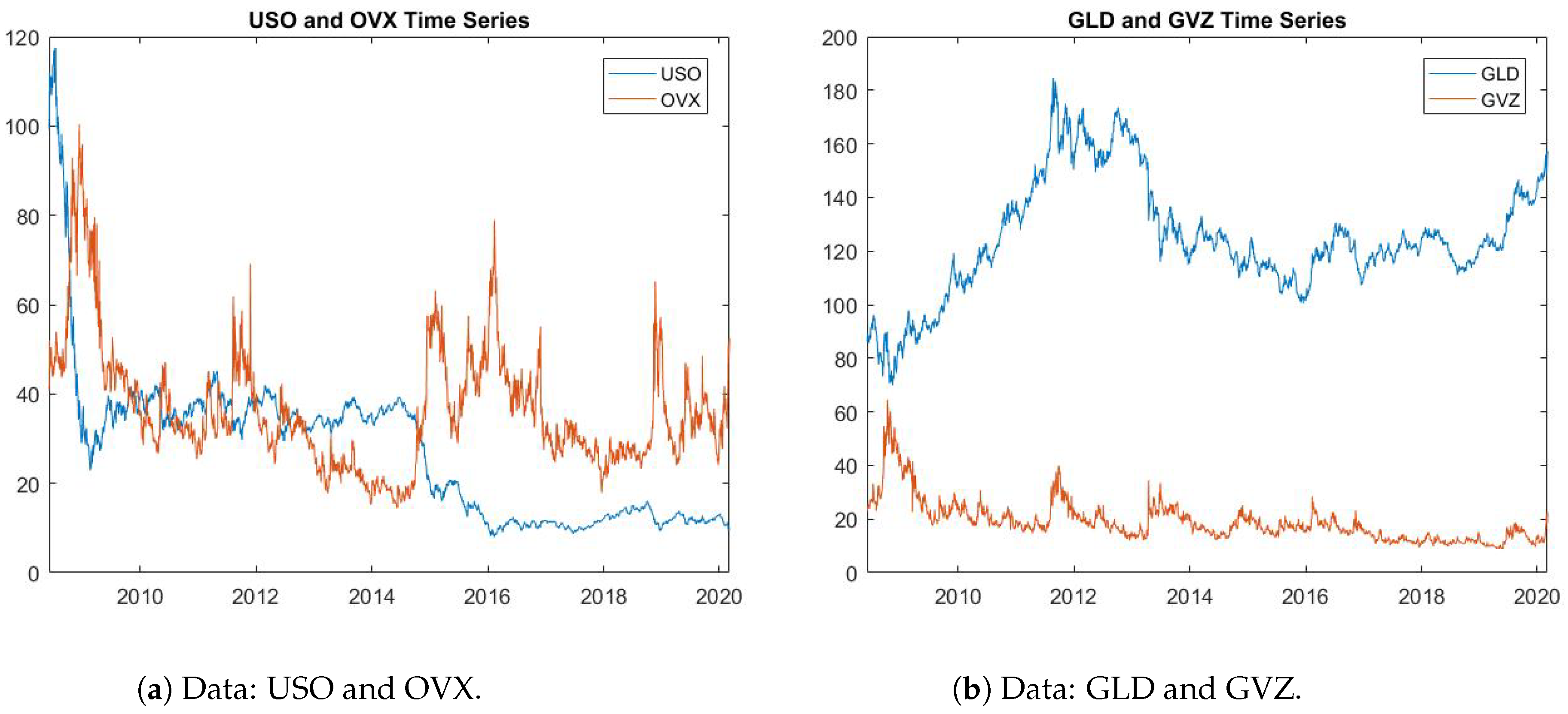
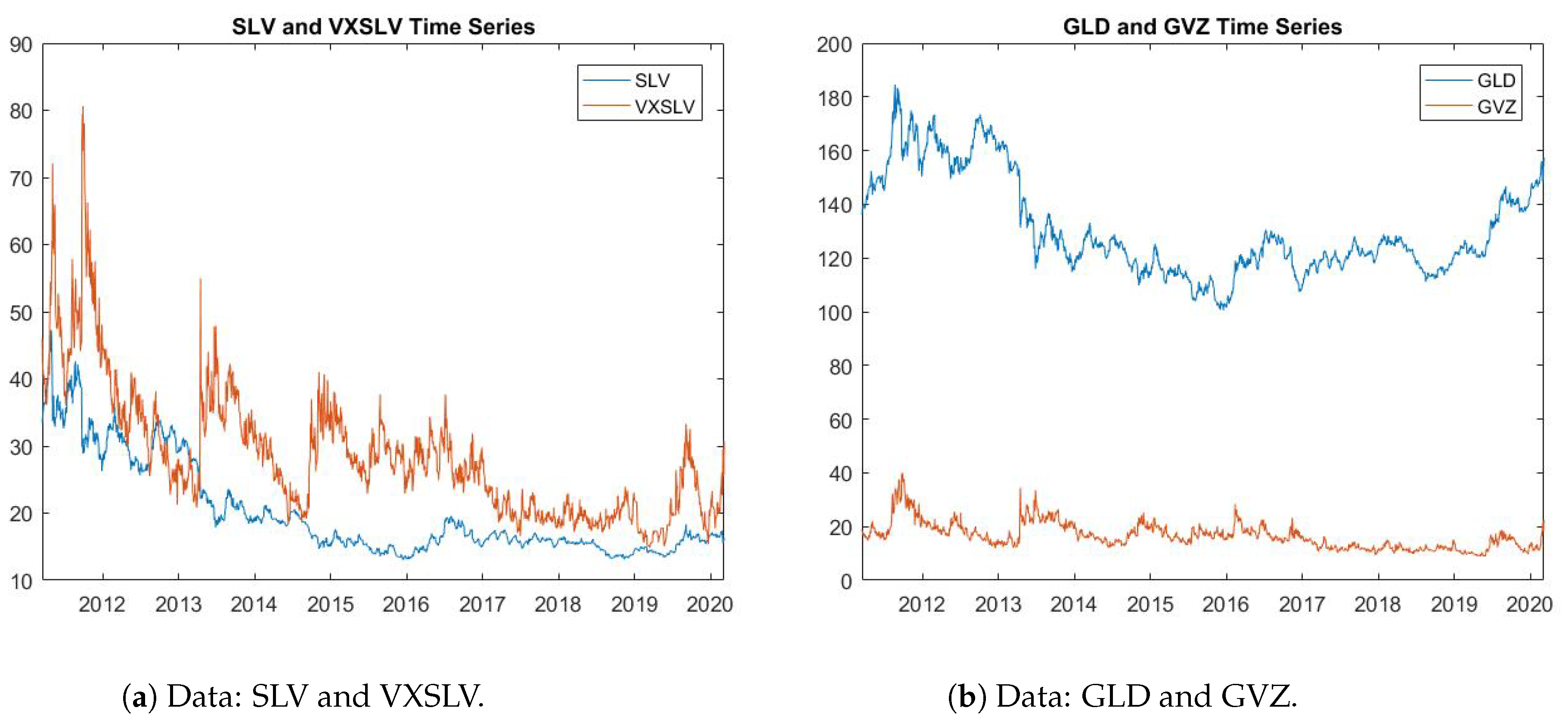
We consider the following pairs of assets and volatilities: The first study is on VIX (S&P 500 Volatility Index) and VSTOXX (Euro STOXX 50 Volatility Index); here, we also use the volatility indexes VVIX and VVSTOXX, respectively. The second group is comprised of USO (Oil ETF) and GLD (Gold ETF), with OVX and GVZ as the respective volatility indexes. The third and final group is made up of SLV (Silver ETF) and GLD, with VXSLV and GVZ as the respective volatility indexes. All these data sets are daily in the period from late 2010 to early 2020.
Our estimation method consists of two stages: we first estimate the parameters in the assets’ data (called drift group), and then the parameters in the assets’ volatilities (called the volatility group). The sample size of the raw data is different across all the assets and volatility indexes. Hence, we must further process the data to better suit our estimation purpose, in particular ensuring that we take only the trading days when both assets and their volatilities can be observed.
Figure 1,
Figure 2 and
Figure 3 depict the pairs of asset data and their volatility indexes. Note that the volatility index data is quoted as annualized volatility multiplied by 100. When we use the volatility index for estimation, we transform the volatility index to daily volatility by dividing by
.
4.2. Estimation of Volatility Group Parameters
The model used for estimation of the “volatility group” parameters in this section is the model with separable spillover effects, described next for completeness.
Recall that Equation (
6) gives us the representation for each principal component that reflects on our mean-reverting 4/2 stochastic volatility model; that is,
, with
defined as
The estimation procedure for this model setup can be summarized as follows. We first transform the data using matrix
to produce the
process following the relationships among
,
and
. Then, we can use the estimation method developed in
Escobar-Anel and Gong (
2020) for each
process. Finally, we recover the parameters for each
process.
4.2.1. Estimation of Matrix and the Scaling Parameters S
In the next sections, we estimate the parameters in the volatility group. The empirical results are summarized in
Table 1. The first step is to estimate matrix
, as it connects log asset prices
and principal components
. Recall that
is an orthogonal matrix comprising the eigenvectors of covariance matrix
. Given daily data, we estimate
by first calculating the empirical covariance matrix
and applying eigenvalue decomposition:
where
is a vector of the eigenvalues of
, and
is the estimate of matrix
. In
Table 1, we include the results for
,
and eigenvalues
from empirical data. Note that
is not unique in that the signs of each element in the matrix can be manipulated such that the column vectors are still the eigenvectors for the corresponding eigenvalues, while
preserves its orthogonality.
As mentioned at the beginning of this section, volatility indexes are a useful proxy for instantaneous volatility; however, they may require scaling adjustment. Let
denote the squared observed volatility indexes data for
n assets. We introduce a scale parameter
to bridge observed volatility indexes’ series
s to theoretical variances via the following relationship:
where
is a diagonal matrix with diagonal vector
. In theory,
is a function of
, see
Luo and Zhang (
2012), and
Zhang and Zhu (
2006), some of which fall into the volatility group and are to be estimated. Hence, devising an estimate that does not depend on these parameters is crucial. We propose an estimate that matches the long-run first empirical moment of both sides of Equation (
16). The long-term average of the left-hand side of Equation (
16) can be directly calculated from squared volatility indexes’ data. The long-term average of the right-hand side may not seem as straightforward, as it deals with a stochastic process. In our definition,
is the diagonal of the covariance matrix and refers to the instantaneous variance process. Therefore, in the long run, the expectation of the variance process should converge to the variance of the underlying asset. Let
denote the empirical long term variance of asset
i, and let
denote the long-term average of the corresponding squared volatility index data. We estimate
as
Substituting Equation (
18) and
back to the right-hand side of Equation (
17), the long-term average is
which matches the left-hand side of Equation (
17) in terms of the long-term average, as
is the eigenvalue of
and converges to
in the long run.
Table 1 also displays the results for
,
and
.
4.2.2. Estimation of Volatility Group
Let
, and let the
j-th eigenvalue of
be defined as
. Then,
is represented by
according to Equation (
17). Suppose
is a series of squared volatility indexes for asset
i observed on
; then, at time
, we have
.
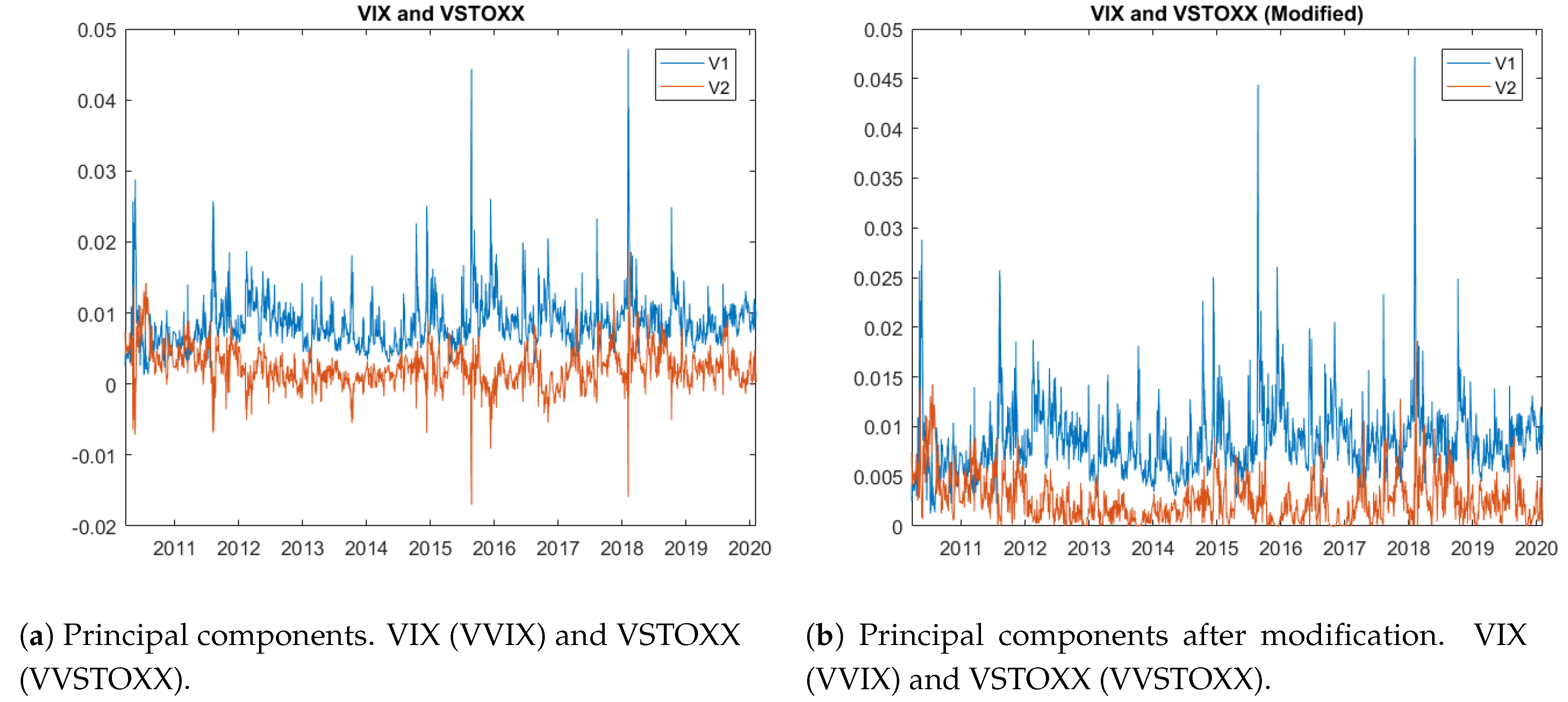
In theory, we expect the
series to be non-negative, since it is related to the series of instantaneous variances
for the underlying assets. In practice, however, we observe inconsistencies in some cases. For example, as
Figure 4a illustrates,
has a number of negative values (labeled by “V2”), which are non-negligible. Next, we perform a preliminary analysis to locate the root of the issue.
To solve the problem of inconsistency without modifying our model, we deal with the negative values as if they are missing values. We thus replace the negative values by the weekly averages centered on those negative values.
Figure 4b illustrates the series of
and
after this modification. Furthermore,
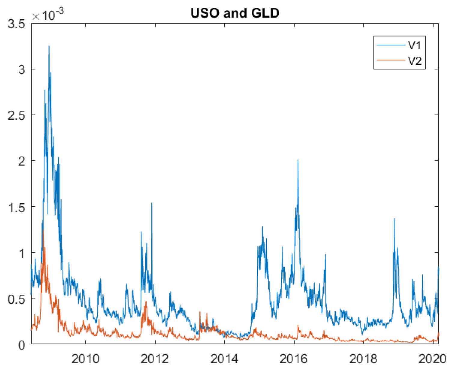
Figure 5 presents two series:
and
after transforming the original OVX and GVZ data. In this case, we do not observe the inconsistency shown in
Figure 4b, which means that the data supports our model. The figure also illustrates the trend as expected, with the first principal component generating the largest variation (
) in asset price compared to the second principal component (
).
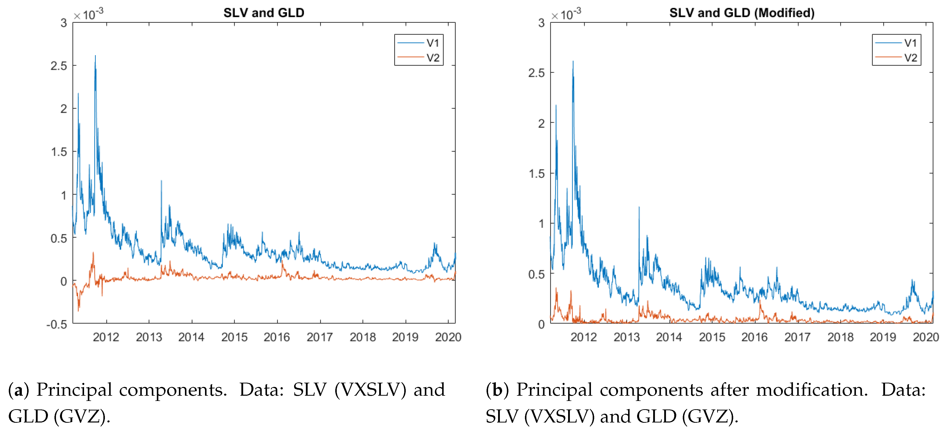
In
Figure 6a, we also observe some inconsistency in silver ETF (SLV) and gold ETF (GLD) data between 2011 and 2012. Given that the correlation between SLV and GLD is large,
series stays close to 0, which implies that the two assets are likely driven by the same random factor. Since the negative values do not appear as often as in
Figure 4a and are close to 0, we simply take the absolute value of the negative values and show the modified series in
Figure 6b.
Now that we have prepared all the data for estimation, we apply the estimation method developed in
Escobar-Anel and Gong (
2020) to
and
to estimate
and
. Note that, in all three scenarios, the minimum of
is approximately zero, which implies that
is 0 as seen from
Figure 4b,
Figure 5 and
Figure 6. Therefore, it is sufficient to model
as a CIR (1/2) process instead of a 4/2 process. On the other hand, the “spikes” occurred frequently in
—labeled as “V1” and shown by the figures—are signals that
should be a 4/2 process given all three pairs of assets-and-volatility index data. Since we assume that
follows a CIR process, we estimate
using maximum likelihood.
Table 2,
Table 3 and
Table 4 list the estimated parameters and their standard errors (s.es) with the chosen data sets for parameters in the volatility group.
The inference on the parameters (asymptotic mean and variance) is performed via parametric bootstrap. In other words, we simulate the corresponding processes with the estimated parameters 1000 times and repeat the estimation procedure for each simulation. In the end, we obtain a pool of 1000 sets of estimates. The law of large numbers suggests that the means calculated from the pool of estimates are the asymptotic means for each estimator. It is interesting to see how the first principal component not only accounts for most of the variation, but it also absorbs the complexity of the problem. In other words. the tables show that the first component requires the advanced 4/2 modeling (i.e., ), while the second component can be better explained with the simpler 1/2 model ().
4.3. Estimation of Drift Group
Similarly, we use the least square approach to estimate parameters in the drift group.
Table 5,
Table 6 and
Table 7 display the results. Some parameters are assessed to be non-significant based on the p-values. We decide to keep all the parameters because our sample sizes are not large enough to draw concrete conclusions on the significance of the parameters.
Note that the estimated parameters reported in the tables are for the parameters of the
and
processes. We can recover the estimates for original parameters using the relationship we defined earlier; that is,
,
, and
. The estimates for the original parameters are reported in
Table 8. The diagonal entries in the
matrices provide information on the mean-reverting speed for all the assets. Note that for the pair SLV and GLD, one of the eigenvalues (
) of
does not satisfy the assumption imposed on the eigenvalues of
, which is a sign that the data does not support this particular model. The correlation coefficients are not included because they are not affected by the transformation.
It is worth noting that
in
Table 8 does not reflect the actual mean-reverting level. Therefore, to determine the mean-reverting level for each asset, we must go back to Equation (
4) and rewrite it in following format:
We can now see that the mean-reverting level is
plus a random component, which we define as
. The long term mean indicated by the model is basically
. We report these estimates in
Table 9 and compare them with the averages calculated from empirical data.
As
Table 9 shows, the estimated MRLs are close to the empirical log price averages, except for the USO case, where the estimated mean is smaller than the empirical mean. This latest point might be due to the impact of the initial value on the stationary value of a 4/2 process. Moreover, the VIX and VSTOXX pair has the largest mean-reverting speed compared to the other two commodity ETF pairs. This is not a surprise, as evidenced by empirical data. Volatility indexes tend to return to the mean faster due to an economic cycle, whilst commodities normally have a longer time horizon to revert to the mean level due to scarcity, demand and supply.
5. Application to Risk Measures
Risk measures in financial risk management are used to determine the minimum amount of capital to be kept in reserve in worst-case scenarios as a way of protecting financial institutions. There are many risk measures in the literature, see, for example,
Artzner et al. (
1999) and
McNeil et al. (
2005), one of which is considered fundamental: Value-at-Risk (VaR), which is a distribution-based risk measure. In other words, a VaR calculation takes into account the distribution of the underlying (VaR is in fact a quantile). It is more robust to outliers than mean and variance.
In this section, we compute the VaR of a portfolio consisting of two assets and a cash account, in line with the previous estimation section. We must first find the distribution of this portfolio, which might not be available due to, in particular, the correlations among the underlyings. In the language of mathematical statistics, we must find the joint distribution of USO and GLD to compute VaR. In general, finding closed-form expressions for the joint distribution of two non-Gaussian stochastic processes is theoretically difficult. In fact, USO and GLD have complex distribution functions under our multidimensional 4/2 model setting. Fortunately, this is feasible in our model, as we can express the joint distribution at any given date of USO and GLD in terms of two independent random variables, which simplifies our problem significantly and allows for the use of c.f.s to compute the properties of the portfolio distribution.
5.1. Portfolio Setup
Suppose that we have a portfolio
consisting of two assets
and
:
where
and
represent the weights of
and
in the portfolio, and
is a cash account with interest rate
r. In a short period of time, we can also write the problem using the self-financing condition and relative portfolio weights
,
and
; that is, the proportion allocated to the assets and cash account, allocations see
Campell et al. (
1997):
Constant allocations will be considered (i.e., constant
), as they constitute the most popular investment strategy in the market, supported by
Merton (
1975). From the process
, we can easily obtain
(
by using Ito’s lemma. When comparing
and
, we observe that only the drift term is adjusted, while diffusion terms stay the same. Assuming that
are modeled by Equation (
2), the log prices
then have the SDE specified in Equation (
4) under the PCSV framework. Moreover, we can also write
in terms of
:
Hence, we rewrite Equation (
20) as follows:
It is known that
and
are linear combinations of two independent stochastic processes or random variables
and
:
We now substitute
and
in Equation (
21) with Equations (
22) and (23):
From Equation (
24), we can conclude that
is also a linear combination of
and
, with adjustment to the drift terms, which does not affect the independent relationship between
and
. We organize Equation (
24) into the following expression:
where
and
are independent, with
where
,
,
,
, and
.
Note that for convenience, we included the growth rate on the cash account into the long-term average of
. From a mathematical perspective,
is constructed based on
, which is the first principal component that determines the most variation among the assets. As a result,
affects the performance of
more than
financially. For this reason, the effect of the growth rate on the portfolio can also be interpreted as if it impacts the long-term average of
. Now, we apply Ito’s lemma to Equation (
25) to obtain the dynamics for
:
where
It is straightforward to find the characteristic function of using the above mentioned results.
5.2. The Density Function of the Portfolio
From Equation (
26), our portfolio now essentially contains two new “assets” that are independent of each other. Thanks to this independence, we can derive the characteristic function as well as the density function of our portfolio. Since our goal is to calculate the VaR, it is convenient to use a density function and integrate numerically. In this section, we list two approaches to obtain such a density function.
5.2.1. Density Function via Convolution
One way in which to obtain the conditional density function for
is via convolution of two conditional density functions for
and
. In probability, if two random variables
X and
Y are independent, with density functions
and
, respectively, then the density for
,
, can be found via convolution; that is,
If
X and
Y have analytical density functions, then the convolution method is straightforward. In our case, we obtain the conditional c.f. first. The Fourier inversion of the conditional c.f. theoretically gives the density function. However, due to the structure of our original c.f. and the approximations, we need to invert both the original c.f. and the approximated c.f.s numerically for the corresponding density functions. For
and
, we can obtain their conditional corresponding density functions
and
by inverting the c.f. of
and
:
We can now write Equation (
32) as a convolution of Equations (
28) and (
29):
A challenging part of this method is that we must first invert the semi-closed c.f.s to obtain the density functions for
and
—artificial assets—which involves approximations. As we have well-developed approximation approaches for
, we can apply the results to obtain the analytic function as an approximation of the c.f. for individual artificial assets and then find the density via Fourier inversion. Then, we can use Equation (
30) to obtain the density of the portfolio. The approximation approaches work well in a parametric region, as demonstrated in
Escobar-Anel and Gong (
2020), for three scenarios (
); the goodness of approximations depends on
.
5.2.2. Density Function via Fourier Inversion
Another, more direct means of obtaining the density function is to apply an inverse Fourier transform to the characteristic function. Before we provide the formula for the characteristic function, we consider the transformation
. By Ito’s lemma, we have
The next corollary explains how to derive the characteristic function.
Corollary 4. Let denote the characteristic function provided in Proposition 2.1 in Escobar-Anel and Gong (2020); then, the characteristic function of is given by the following equation:where , Let
p denote all possible values in the domain of
; the density function hence follows from
It can be seen that the c.f. of the portfolio does not have a closed-form representation, since it is a product of semi-closed c.f.s (
). As a result, we could use the approximations developed in
Section 3.3.
5.2.3. Numerical Implementation of Selected Method
The Fourier inversion method and the convolution method theoretically yield the same density function for the portfolio. Moreover, in a portfolio that only consists of two (artificial) risky assets, both methods are not complicated to implement. We implement the convolution method with partial simulation for applications with only two assets. However, it would be more efficient to use the Fourier inversion method when the portfolio has a large pool of assets (e.g., over 100). To see this, note that, for assets, the convolution method involves the simulation of n processes with integrations; in contrast, the Fourier inversion method reduces the number of integrations to just one.
We summarize the numerical implementation to compute the conditional density function of the portfolio in the following steps:
Step 1: Simulate two CIR processes and and compute for and .
Step 2: Invert the c.f.s obtained in Step 1 to obtain and .
Step 3: Numerically integrate the product of the conditional density of and for the conditional density function of .
Even though we use partial simulation to obtain the density function of the portfolio, partial simulation is not time-consuming, as efficient methods exist to simulate CIR processes; see, for example,
Andersen (
2007). Moreover, both the convolution method and the direct Fourier inversion method require either fewer simulations or no simulations (via approximations), compared to a full simulation approach, which would require the simulation of four processes. In the case where semi-closed c.f.s are involved, we would only need to simulate at most
processes (
for
process), instead of a simulation of the
processes altogether (
processes). Most importantly, thanks to PCA decomposition, we would likely need
m such volatility drivers to explain the SC of
n assets with
. This means a substantial reduction in computational complexity (partial, simulations, integrations or approximations).
In summary, under a PCSV framework, partial simulation is a good choice in terms of efficiency. The PCA reduces computational complexity, as fewer diffusions may be required to explain the variation of all assets. Our approximations further improve the efficiency for computing the c.f.s with analytic functions.
In the next application section, we apply the convolution method from
Section 5.2.1 to compute the VaR at popular quantile
(
).
5.3. The VaR for a Portfolio of USO and GLD
In this section, we consider a pair of risky assets: USO and GLD, and we study
under an investment strategy: equally weighted risky assets only (
)
2. These have been proven to be robust and reliable strategies in the seminal work of
DeMiguel et al. (
2009). In
Table 10, we report the
values and their s.es. We consider a well-known asymptotic result for quantiles to calculate the s.es for
as derived in
Stuart et al. (
1994):
where
is the quantile of the portfolio distribution (in this case, it is
);
n is the sample size, and
is the probability distribution function (density function) evaluated at
.
Case:
In this case, we use the information from
Table 1b,
Table 3 and
Table 6 to obtain parameters that generate
or
.
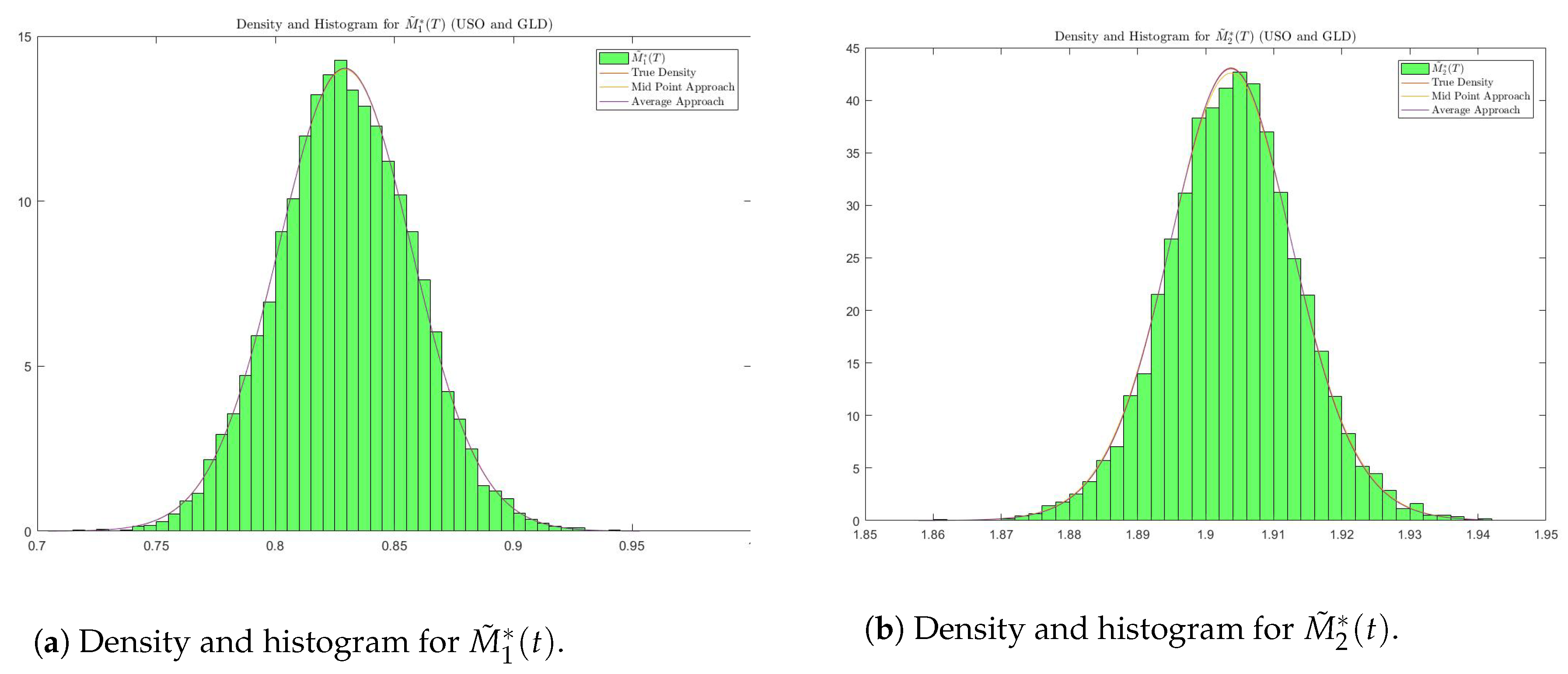
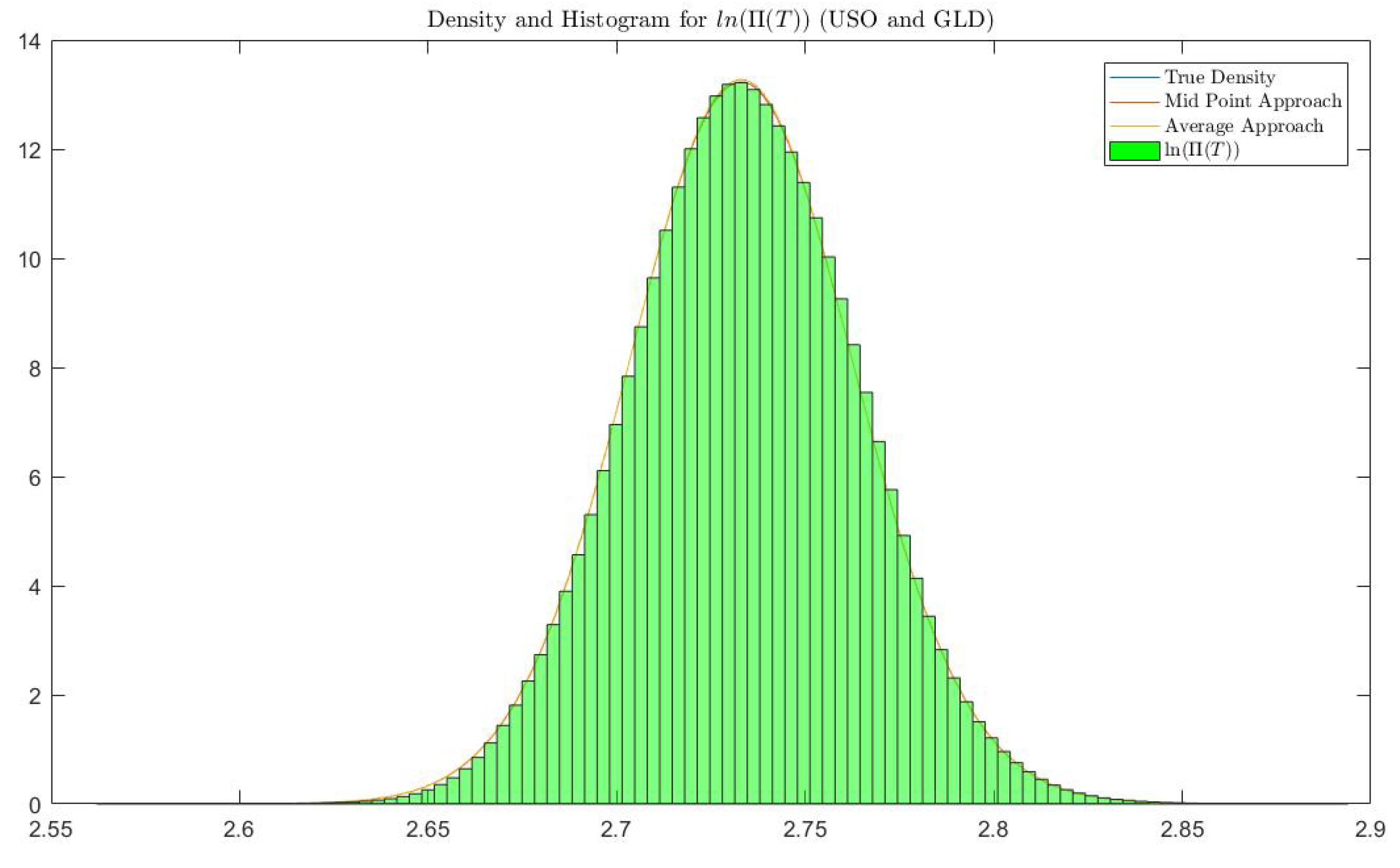
Figure 7 and
Figure 8 confirm that density functions from theory are in line with the simulations. We compute and compare
values from four sources: simulation of the portfolio (Simulation), density function without approximation (Density w/o Approximation), approximated density function using the midpoint approach (Approx. Density (M)) and approximated density function using the average approach (Approx. Density (A)).
We use linear interpolation here to calculate the quantile if falls between two critical levels calculated from histogram and density functions. Standard errors are reported in parantheses.
6. Conclusions
This paper studied the properties of a multivariate mean-reverting 4/2 stochastic volatility model based on principal component decomposition. In particular, we studied the variance and covariance processes as well as several submodels of interest to the industry (e.g., separable or no spillover effects, multivariate mean-reverting Heston models). We also obtain an expectation representation for the c.f. of the asset prices with respect to the paths of the stochastic volatility process. Two closed-form approximations to the c.f. are presented in
Section 3, these are the first efficient calculations of c.f. for multivariate mean-reverting stochastic covariance models. In
Section 4, we implemented a two-step estimation methodology to three sets of data involving two asset classes, commodities and volatility indexes. The study confirms stylized facts commonly attributed to commodities, like spillover effects, are also observed in the joint dynamic of volatility indexes, which has not been previously reported; it also displays the role and need of scaling parameters between instantaneous variance and volatility indexes in a multidimensional setting.
In
Section 5, we further tested our approximation methods in a risk management setting by computing one of the most popular risk measures, namely, VaR. Since VaR is a distribution-based risk measure, our analysis confirms the effectiveness of the c.f. approximations in a multidimensional setting for a portfolio of advanced stochastic processes. Although our analysis was in two dimensions, the methodology is transferable to any dimension, e.g., a portfolio with a large number of underlying assets. In such case, the average-based approximation can greatly save time in calculating distribution-based risk measures, the alternative is the MontCarlo simulation of a high number of continuous-time processes with the subsequent loss in precision.


