Bankruptcy Prediction with a Doubly Stochastic Poisson Forward Intensity Model and Low-Quality Data

Abstract

With the record high leverage across all segments of the (global) economy, default prediction has never been more important. The excess cash illusion created in the context of COVID-19 may disappear just as quickly as the pandemic entered our world in 2020. In this paper, instead of using any scoring device to discriminate between healthy companies and potential defaulters, we model default probability using a doubly stochastic Poisson process. Our paper is unique in that it uses a large dataset of non-public companies with low-quality reporting standards and very patchy data. We believe this is the first attempt to apply the Duffie–Duan formulation to emerging markets at such a scale. Our results are comparable, if not more robust, than those obtained for public companies in developed countries. The out-of-sample accuracy ratios range from 85% to 76%, one and three years prior to default, respectively. What we lose in (data) quality, we regain in (data) quantity; the power of our tests benefits from the size of the sample: 15,122 non-financial companies from 2007 to 2017, unique in this research area. Our results are also robust to model specification (with different macro and company-specific covariates used) and statistically significant at the 1% level.

1. Introduction

In the world ravaged by the pandemic, with a fragile macro-economic outlook, low interest rates, and record high leverage, any academic research on bankruptcy is welcome. As the authors of this paper, we are neither professionally prepared nor interested in the debate on the degree of macro fragility or the effectiveness of the unprecedented stimulus packages adopted worldwide. Mentioning the unparalleled global leverage positions or the global health crisis, we merely acknowledge the emergence of the almost unmatched global uncertainty. In contrast to more optimistic views, exemplified by the stock exchange post-COVID-19 valuations, we believe the uncertainty is the only certain thing around us these days. Understanding the process of going down (in these circumstances) seems to us more than critical. Throughout this paper, bankruptcy and default are used interchangeably.

Below are some universally available leverage statistics (Altman 2020). Global non-financial corporate debt increased from the pre-Global Financial Crisis level of $42 trillion to $74 trillion in 2019. The government debt position more than doubled from $33 trillion in 2007 to $69 trillion in 2019. Even the financial sector increased its leverage from the record high pre-crisis level to $62 trillion. Households increased their debt globally from $34 trillion to $48 trillion. With the exception of the financial sector, debt also grew in relation to global GDP. It increased to 93% for non-financials (up from 77%), to 88% for governments (up from 58%), and to 60% for households (up from 57%). Despite this, as Altman (2020) notes, the corporate high-yield bond default rate was surprisingly low at 2.9% in 2019, below a 3.3% historic average, the recovery rate of 43.5% was quite in line with the historic average of 46%, with the high-yield spreads lagging behind historic averages, too. Consequently, Altman believes that the pre-COVID-19 debt market, in contrast to the current state, was still at a benign cycle stage. However, the very levels of debt globally, coupled with the increased appeal of a very long end of the yield curve and a massive increase in the BBB issuance, makes the debt markets and the global economy quite vulnerable, even without the health crisis. The unconventional monetary policies and the low interest environment also lead to the proliferation of “zombie” firms. Regardless of the precise definition, these companies are kept alive rather artificially thanks to the availability of cheap debt. Banerjee and Hofmann (2018) estimate as much as 16% of US listed firms may have “zombie” status—eight times more than in 1990. Acharya et al. (2020) estimate that 8% of all loans may also be infected with the “zombie” virus. Needless to say, COVID-19 and the resultant generous governmental relief packages do not help mitigate the problem.

Bankruptcy research, in all its guises, has been truly impressive and has produced many insightful results for some decades now. Such results include the classical structural models of Merton (1974), Fischer et al. (1989), and Leland (1994), numerous reduced-form models ranging from the simple scoring methods of Beaver (1966, 1968) and Altman (1968), qualitative response models, such as the logit of Ohlson (1980) and probit of Zmijewski (1984), to the third generation of the reduced form, the duration-type models of, for e.g., Shumway (2001), Kavvathas (2000), Chava and Jarrow (2004), and Hillegeist et al. (2004). They all propose various and divergent econometric methods and methodological approaches, with an impressive sectorial and geographic empirical coverage (see Berent et al. 2017).

To discriminate healthy from unhealthy firms is one challenge; to predict the (multi-period) bankruptcy probabilities is another. One way to address the problem is to model default as a random counting process. A Poisson process is such an example. In the bankruptcy literature, it is the Poisson process with stochastic intensities that is frequently used. In the doubly stochastic setting, the stochastic intensity depends on some state variables which may be firm-specific or macroeconomic, also called “internal” or “external” in the works on the statistical analysis of the failure time data (Lancaster 1990; Kalbfleisch and Prentice 2002). We adopt the Duffie–Duan model, as described in Duan et al. (2012), who, with their forward intensity approach and the maximum pseudo-likelihood analysis, follow in the footsteps of Duffie et al. (2007). In 2007, Duffie et al. (2007) first formulated a doubly stochastic Poisson multi-period model with time-varying covariates and Gaussian vector autoregressions. Duan et al. (2012) resolve some specification and estimation challenges inherent in Duffie et al. (2007). With their forward intensity concept, Duan et al. (2012) no longer need a high-dimension state variable process to be assumed, but instead use the data known at the time of making predictions. Both Duan et al. (2012) and Duffie et al. (2007) are well grounded in the doubly stochastic hypothesis literature debated in, for e.g., Collin-Dufresne and Goldstein (2001), Giesecke (2004), Jarrow and Yu (2001), and Schoenbucher (2003).

Duffie et al. (2007) apply their model to US-listed industrial firms. Duan et al. (2012) use also US public companies traded on NYSE, AMEX, and Nasdaq. Other researchers use the Duffie–Duan model to assess the default risk of public firms and/or in the context of developed (e.g., Caporale et al. 2017), or emerging markets (Duan et al. 2018). In this paper, we demonstrate that the Duffie–Duan model not only successfully describes a default process for public companies from developed countries with well-functioning capital markets, but is also equally successful in the context of privately owned equity markets with frequently patchy, low-quality data, operating in an emerging market characterized by lower transparency and governance standards (Aluchna et al. 2019). Compared to Duan et al. (2012) and Duffie et al. (2007), we apply the model to a significantly larger dataset of over 15,000 firms. As it is the applicability of the model rather than the discrimination itself that is our priority, we are not optimizing any cut-off point to maximize the accuracy of discrimination (typically made within an in-sample estimation context), but we make use of the out-of-sample accuracy measure calculated across all cut-off points, as is done in the context of the ROC analysis.

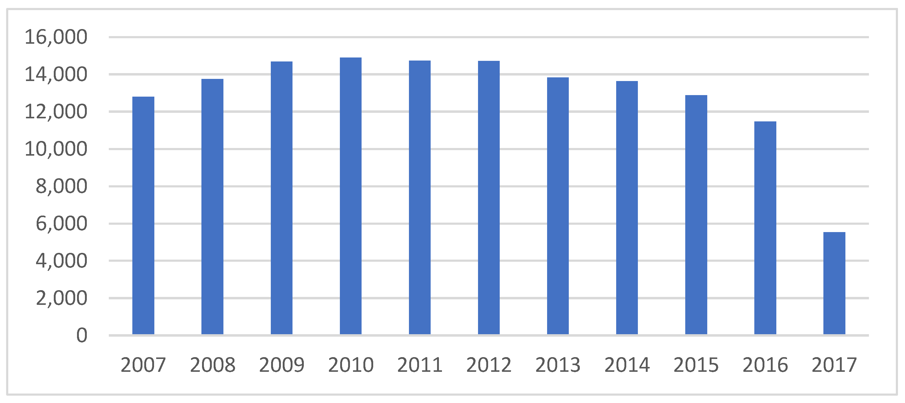
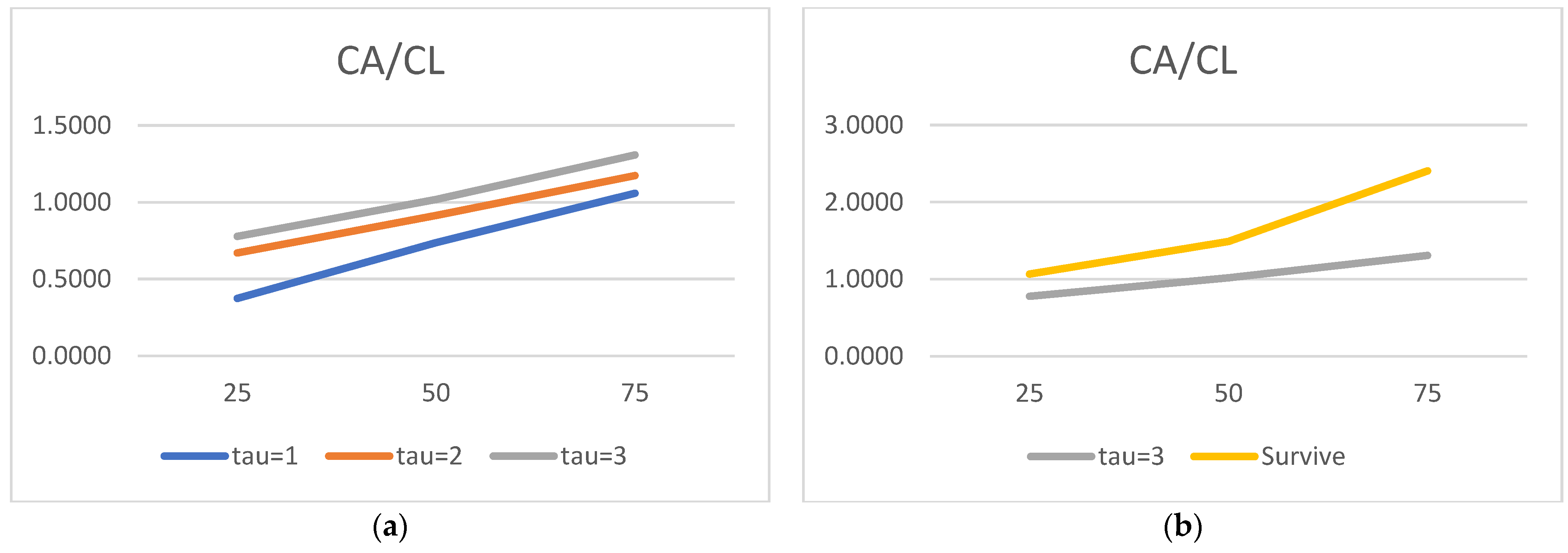
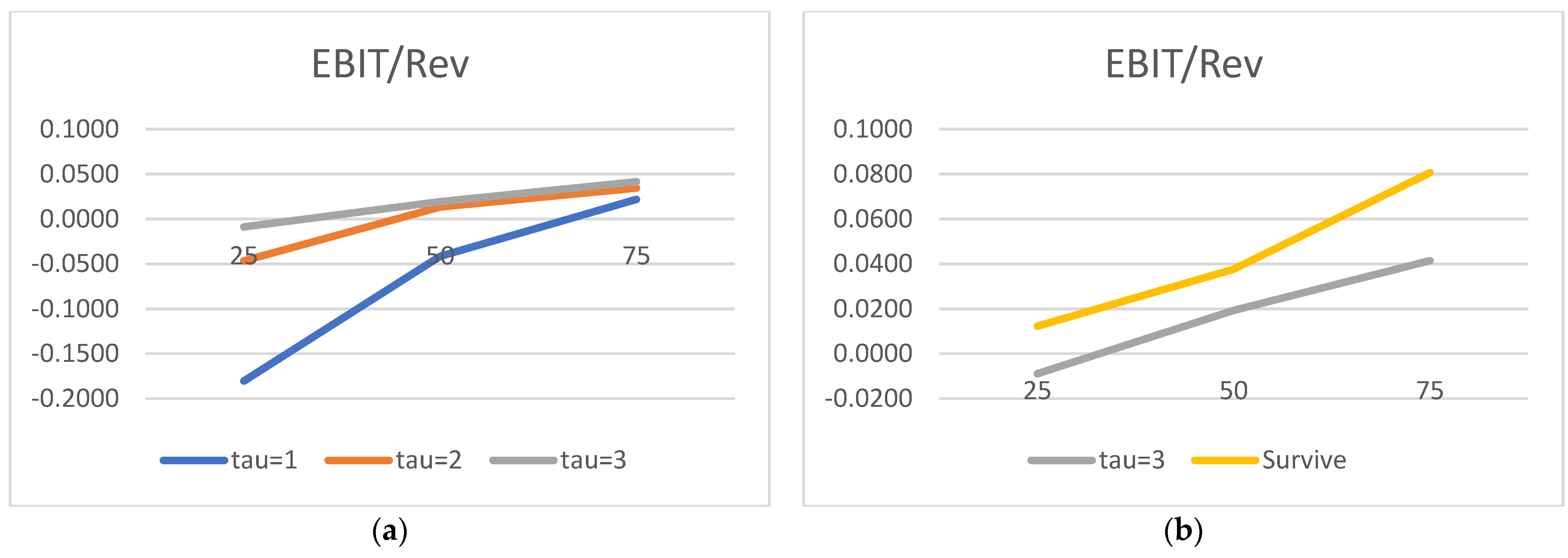
First, we collect a unique dataset for as many as 15,122 non-financial companies in Poland over the period 2007–2017. We make a huge effort to cross-check and cleanse the data so that the intricate estimation procedures could be run on this (initially) patchy input. Then, we document the performance differential (in the form of financial ratios) between the healthy and the (future) bankrupt firms one, two, and three years before default. In the next stage, company-specific variables (liquidity, profitability, leverage, rotation, and size) and macroeconomic variables (GDP growth, inflation, and interest rates) are used as state variables to estimate the default forward intensity employed in the doubly stochastic Poisson formulation. Partly due to the size of the dataset, we believe, we are able to exploit the differences between the attributes of the two groups. What we lose in the (data) quality, we seem to regain in (data) quantity. Our results surpassed our expectations. Not only are the estimated covariate parameters in line with the expectations and the literature, but the out-of-sample accuracy ratios produced—85% one year before default, 81% two years before default, and 76% three years before default—are at least as high, if not better, than those obtained for the high-quality public companies from developed countries. All our results are statistically significant and robust to the (state variable) model specification.

We hasten to repeat that this paper is not about searching for the determinants of default, neither is it about the maximization of the discrimination power between the two groups at any optimal cut-off point. In particular, we are not interested in artificially lifting up the in-sample fit. The main objective is to prove that the doubly stochastic Poisson model can be successfully used in the context of low-quality data for non-public companies from emerging markets. We believe this objective has been fully achieved. We are not aware of any similar effort in this area.

The rest of the paper is organized as follows. Below, still within the introduction section, we briefly introduce Poland’s bankruptcy law, an important ingredient, given the recent overhaul of the legislation framework. In the Materials and Methods section, we describe our unique dataset, introduce the model and the micro and macro covariates, and then we define the accuracy ratio, our preferred goodness-of-fit measure, the ROC curves, and the statistical tests applied. In the Results section, we first produce and comment on the descriptive statistics, separately for survivors and defaulters, one, two, and three years prior to bankruptcy. We then analyze the estimated covariate parameters and accuracy ratios, in- and out-of-sample. The critical discussion of our results, in the context of the literature, follows in the Discussion section. We conclude with some proposals for future research in the Conclusions section.

Poland’s Bankruptcy Law

With regard to Poland’s bankruptcy law, it was not until 2003, nearly one and a half decades after the end of communism in Poland, that the new legislation came into force. The new Bankruptcy and Rehabilitation Act replaced the pre-war ordinance of the President of the Republic of Poland, dated as far back as 1934. The new law was universally praised for bringing together, under one umbrella, two separate bankruptcy and restructuring (composition) proceedings, hitherto governed by the two separate legal acts. It is paradoxical that the essence of the latest changes in Poland’s bankruptcy law consisted in the carving out of the rehabilitation part into once again a separate Restructuring Act, which came into force in 2016. Apart from some substantial changes to the proceedings (e.g., the extension of both the time as well as the list of persons entitled/obliged to file for bankruptcy), the new law gave a debtor the option to choose, depending on the severity of insolvency, between four distinct ways to reach an agreement with the creditors. Given the discontinuity/alteration of the default definition brought upon the changes in the legal frameworks, care must be taken while conducting research in the bankruptcy field in Poland.

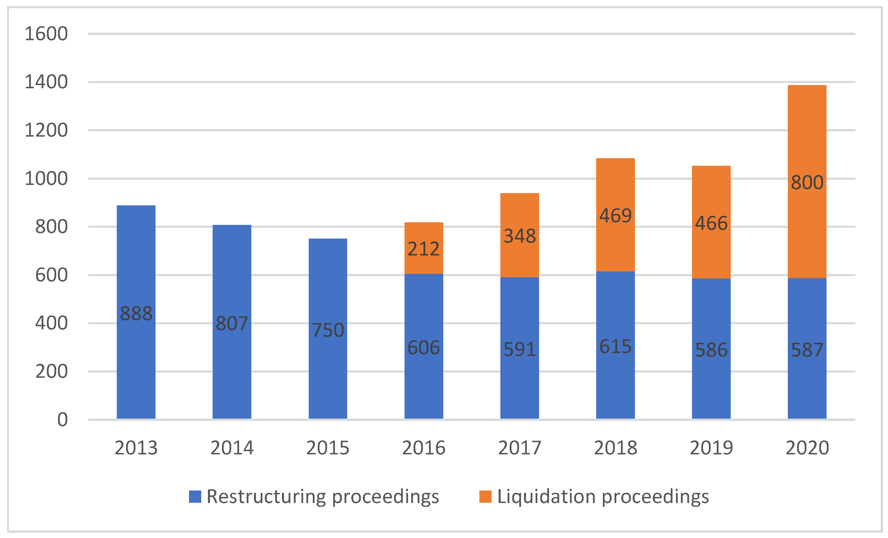
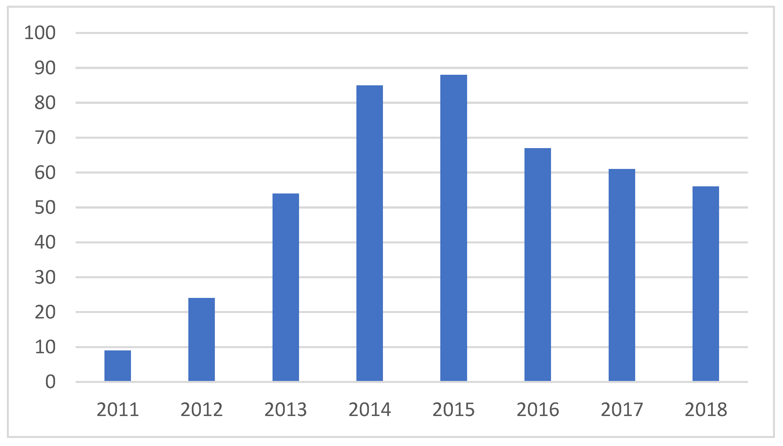
The motivation for the new 2016 law was clear, as the number of liquidation proceedings dwarfed the restructurings by the ratio of 5:1. As Figure 1 illustrates, the effort was worth making, as the number of restructuring proceedings has significantly improved ever since. In 2020, restructuring proceedings outnumbered liquidations, partly due to COVID-19-driven regulations. The trend is generally assumed to remain even after the pandemic.

2. Materials and Methods

2.1. Data

2.1.1. Companies’ Financial Data

Our sample is quite unique in that it is large and dominated by non-public companies. It consists of two subsets. The former is the dataset of financial accounts, and the latter is the dataset on default events. Both are provided by Coface Group, the world’s leading credit insurance provider and the owner of sensitive data on defaulters. Other data on, for e.g., macro statistics are obtained from publicly available sources such as Statistics Poland (GUS).

As for companies’ financial statements, we assembled financial accounts for as many as 15,122 non-financial Polish companies. According to the Statistical Classification of Economic Activities in the European Community (NACE), 39.8% of our companies come from manufacturing, 30.8% represent the wholesale and retail trade, and the repair of motor vehicles and motorcycles, 12.2%—construction, 5.5%—transportation and storage, 2.8%—information and communication, 2.7%—professional, scientific, and technical activities, and 1.7%—other. All our entities are limited companies, with limited liability companies outnumbering joint stock companies by the ratio of 5:1. The dataset consists of 193,420 company periods from 2006 to 2018. We concede the data are of poor quality in that many missing cells are encountered or contradictory records reported (e.g., subtotals in the balance sheets do not add up). We made a substantial effort to validate, cross-check, and, if necessary, correct the dataset. As a result, we identified 143,451 useable annual company-years, i.e., a modest 73% of all company-years possible assuming all companies produced annual numbers for 2006–2018. Given the minuscule size of the 2006 and 2018 sub-samples, we arbitrarily excluded these years from our sample (see Figure 2). Consequently, when the period of analysis is limited to 2007–2017, the completeness of our dataset significantly improves to 86%. We regard this as satisfactory, as 100% is impossible by definition—some entities went down or exited for any other reason during the sample period. As shown in Figure 2, the number of company-years decreases towards the end of the period, which we associate with the fact that many non-public companies publish their accounts with a big lag. Moreover, some financial accounts arrive in multi-year packages, caused by bad release timing (clearly the company’s fault) or for poor data-collection reasons, which may well be beyond the company’s control. The low quality of the data is by no means disheartening. Quite the opposite. To be able to prove the applicability of the doubly stochastic Poisson process to non-public companies’ data characterized by poor quality, frequently susceptible, and incomplete inputs does lie at the heart of this research, and as such, present a challenge rather than a problem.

Table 1. The number of company-years in the sample 2007–2017.

Year	No. of Annual Financial Statements	Year	No. of Annual Financial Statements
2007	12,798	2013	13,834
2008	13,756	2014	13,631
2009	14,483	2015	12,883
2010	14,887	2016	11,470
2011	14,729	2017	5525
2012	14,712

provides an accurate number of available company-years for each year from 2007 to 2017. The annual frequencies between 2007 and 2016, ranging between 11,470 in 2016 to 14,887 in 2010, are rather stable.

2.1.2. Bankruptcy Events

As for default events, we assembled various data subsets from Coface. Firstly, we obtained a list of 1240 companies ticked as bankrupt by Coface itself. Upon closer scrutiny, we realized the definitions of bankruptcy underpinning the tick were different from one firm to another. For example, in some instances, the company was implicated as bankrupt after the court decision, but in others, after a mere petition to court. Consequently, we also collected a separate dataset (from Coface) of 4095 events related (in any way) to the bankruptcy process. The list covers as many as 41 different, typically legal, categories, such as:

• Filings of a request with a court (by a creditor or a debtor, when applicable) to initiate either bankruptcy proceedings or one of many different restructuring/composition/rehabilitation proceedings;
• Different court decisions made at any different stage, e.g., a court approval (of one of many different arrangement schemes reached by the parties), a dismissal of the bankruptcy petition, a refusal to open restructuring proceedings, a discontinuation of proceedings, etc.

The list includes rather vague events coded by Coface as “bankruptcy” or “other bankruptcy event”, too. For some reason (unclear to us and not explained by the data provider), the events recorded come mainly after 2003, with the highest frequencies after 2010. We subsequently verified that the “bankruptcy” events affected as many as 1240 different companies—the number of bankrupt firms originally identified by Coface. Again, instead of being disheartened by the vagueness and proliferation of different default events not untypical of non-public companies, we were rather determined to select the best event definition, most coherent across time, introducing the least heterogeneity into already high noise brought about by the poor quality of the financial data. The price we were prepared to pay was the reduction in the number of defaulters. A structural legal shift in the Polish bankruptcy law from 2016 onward made some “bankruptcy events” disappear. Other events (related to restructuring proceedings in particular) were only defined in 2016. Eventually, we decided to select the event, coded by Coface as 736, to mean “the declaration of bankruptcy to liquidate the debtors’ assets”. The event was identified for 455 companies from 2007 onwards, with only a few cases of registered liquidation recorded before 2012. Figure 3 shows that the default data are mostly represented by the last few years with no sign of structural change around 2015–2016. In summary, we used the 2007–2017 period for financial statements, and 2008–2018 for the information on default events. The financial statements one, two, and three years prior to the default event are referred to as tau = 1, tau = 2, and tau = 3.

2.2. Model

2.2.1. A Poisson Process

A Poisson process is a simple stochastic process widely used in modeling the times at which discrete events occur. It can be thought of as the continuous-time version of the Bernoulli process. In contrast to the known average time between events, the exact timing of events in a Poisson process is random. The process does not have memory, as the arrival of an event is independent of the event before. A Poisson process is a non-explosive counting process M with deterministic intensity λ, such that

$$\underset{0}{\overset{t}{{\displaystyle \int }}}{\lambda }_{s}ds<\infty$$

(1)

with the property that, for all t and s > t, the random variable M_s-M_t has the Poisson distribution with parameter

$$\underset{t}{\overset{s}{{\displaystyle \int }}}{\lambda }_{u}du$$

(2)

If a random variable N with outcomes n = 0, 1, 2, … has the Poisson distribution with parameter β, then the probability of n occurrences equals:

$$P\left(N=n\right)=e^{-\beta }\frac{{\beta }^n}{n!}$$

(3)

Consequently, the times between arrivals are independent exponentially distributed with mean 1/λ.

We talk about the doubly stochastic Poisson process when the default intensity is stochastic and its intertemporal variation is allowed to depend on observable or unobservable state variables X_t that are linked to the probability of default. Hence, under a standard doubly stochastic assumption, firms’ default times are correlated only as implied by the correlation of factors determining their default intensities. The conditional probability of default within s years is then

$$q\left(X_t,s\right)=E_t[{{\displaystyle \int }}_t^{t+s}{e}^{-{{\displaystyle \int }}_t^z\lambda \left(u\right)du}\lambda zdz|X_t]$$

(4)

Thanks to the doubly stochastic assumption, the dynamics of the state variables are not affected by default and the estimation of the model parameters is rather simple. The maximum likelihood estimator of the default probability can be obtained from the separate maximum likelihood estimations of a vector determining the dependence of the default intensity, and a vector determining the time-series behavior of the underlying state vector X_t of covariates.

Duffie et al. (2007) go one step further and estimate the probabilities of default over several future periods. For that, they need to know the stochastic process λ_t, or to understand the time-series dynamics of the explanatory state variables. Of many potential candidates for the specification of the behavior of X_t, they choose a simple Gaussian vector autoregressive model. Subsequently, they propose a maximum likelihood estimator, which, under some conditions, is shown to be consistent, efficient, and asymptotically normal.

The problems associated with the uncertain knowledge of the future values of state covariates and a potential misspecification of the model is overcome by Duan et al. (2012). Instead of modeling λ_t as some functions of state variables X_t, they propose directly a function f_t(τ) of state variables available at time t and the forward starting time of interest, τ. Following Duan et al. (2012), we also assume f_it(τ), for the i-th firm, to be

$$f_{it}\left(\tau \right)=e^{{\alpha }_0\left(\tau \right)+{\alpha }_1\left(\tau \right)x_{it,1}+{\alpha }_2\left(\tau \right)x_{it,2}+\dots +{\alpha }_k\left(\tau \right)x_{it,k}}$$

(5)

If τ = 0, our forward intensity set-up is the same as the spot intensity formulation of Duffie et al. (2007). The forward intensity method allows estimating future default probabilities without explicitly simulating the high-dimensional state variable process, hence only the data known at the time of performing the prediction are used. Thanks to the pseudo-likelihood function, the estimation of the forward default parameters are unrelated to each other. Being a variant of a standard doubly stochastic assumption, firms’ survival and default probabilities are assumed to depend upon internal or external factors. Any dependency may only result from sharing of the common macro-economic factors and/or any correlation among the firm-specific attributes.

2.2.2. Covariates

The approach to the selection of a set of covariates differs widely. Duffie et al. (2007) mention several variables (e.g., 10-year Treasury yield, personal income growth rate, GDP growth rate, average Aaa-to-Baa bond yield spread, firm size), yet in the final analysis they use only four: distance to default, the three months Treasury bill rate, the (trailing) one-year return on both the S&P 500, and the stock. Their repeated emphasis on the inadequacy of distance to default, which is nothing but a volatility adjusted leverage measure based on Merton (1974), may suggest the comprehensive selection of covariates is not the main priority for Duffie et al. (2007), as long as they identify a model outperforming one that is solely dependent on the distance-to-default itself. Duan et al. (2012) are more generous in the selection of covariates. On top of the variables used in Duffie et al. (2007), they use the cash-to-assets ratio, net income-to-assets ratio, a firm’s market equity value, P/BV, idiosyncratic volatility, etc. Other traditional firm-level risk factors such as leverage, profitability, growth, or liquidity, each in many different formats, are also available. An increasing consensus among researchers exists that adding macro variables to the company-specific covariates improves prediction (Beaver et al. 2005; Shumway 2001; Berent et al. 2017).

Remembering the objective of this paper is to show the applicability of the doubly stochastic Poisson model to a large dataset of low-quality corporate data from emerging markets, we are less preoccupied with the optimal selection of the state variables. Quite the opposite. Knowing the doubly stochastic assumption may, by definition, inadequately represent the default clustering, we opted to enlarge the size of our input beyond Duan et al. (2012). Multicollinearity-type problems that result from the presence of correlated covariates are not our major concern. Consequently, we chose five company-specific areas: liquidity, profitability, leverage, size, and rotation to be represented by two ratios each. The macro variables selected (GDP growth, interest rates, and inflation) are fairly standard, too.

Table 2. The list of firm-specific and macro state variables.

Micro/Macro	Variable	Symbol	Definition
Micro	Liquidity	Cash/TA	Cash and cash equivalents to total assets
		CA/CL	Current assets to current liabilities
	Profitability	NP/TA	Net profit to total assets
		EBIT/Rev	Operating income to revenue
	Leverage	ND/EBIT	Interest bearing liability minus cash and cash equivalents to operating profit
		ND/E	Interest bearing liability minus cash and cash equivalents to equity
	Rotation	Rev/STR	Revenue to short-term receivables
		Rev/TA	Revenue to total assets
	Size	TA	Total assets
		Rev	Revenue
Macro	Gross Domestic Product growth	GDP	Gross domestic product
	Inflation	CPI	Consumer price index
	Interest Rates	WIBOR3	Three-month WIBOR

presents the list and the definitions of the state variables used.

2.3. Accuracy Ratio

The choice among so many “goodness-of-fit” measures in reporting empirical results is critical in the default literature. The ambiguity surrounding this choice may indeed result in major confusion. It should certainly be driven by the research objective and the costs of misclassification. For example, if the priority is to let no (future) bankrupt firm to be treated as healthy, then the count of false negatives is pivotal. Even then, it is not obvious how to report it in relative terms: as the percentage of all bankrupt firms—a so-called false negative rate, or as the percentage of all firms diagnosed as healthy—a so-called false negative discovery rate. A very low false negative rate value may not correspond to a low false negative discovery rate value. Moreover, if one wanted to maliciously report a close to zero false negative rate, one should classify all (most) firms as bankrupt. A different measure, a so-called accuracy rate, takes into account the correct classification of both healthy and unhealthy firms. One should be warned, however, that in an unbalanced population (sample), with the positives being outnumbered by the negatives (as frequently happens), the simple allocation of a negative rating to all objects would, again, produce a very high success ratio.

The almost unparalleled richness of the vocabulary used in this context, a legacy of the binary classification being popular in so many areas (e.g., medicine, epidemiology, meteorology, information theory, machine learning, or methodology) makes the confusion even bigger. For example, depending on the context:

• A true positive rate (a percentage of all positives being diagnosed as positive) may also be referred to as sensitivity, recall, or power;
• A false negative rate (a percentage of all positives being misclassified) can also be called a miss rate, or beta;
• A proportion of negatives being misclassified as positives is referred to as false positive rate, false alarm probability, fall-out, or alfa;
• A proportion of all negatives being correctly tagged as negative is also known as a true negative rate, or specificity.

Similarly,

• A percentage of true positives in the group of all positive designations is called either a positive predictive value, a post-test positive probability, or simply precision;
• Accordingly, a percentage of diagnosed negatives which are indeed negative is known as a negative predictive value (NPV), or a post-test negative probability;
• The ratio of misclassified negatives, in relation to all those positively diagnosed, is referred to as a false positive discovery rate; and
• The ratio of misclassified positives, in relation to all those negatively diagnosed, is referred to as a false negative discovery rate, or a false omission rate.

The list of different names seems virtually endless, and so is the scope for confusion, even if there was clarity in what one really would like to optimize. A classification success of 95%, for example, may therefore mean many different things depending on how the success is defined. In many contexts, a high success is guaranteed with little or no effort. The topic of how the classification success should be measured certainly deserves separate treatment, not only for its linguistic capacity. The wide confusion surrounding the reported “accuracy” of various COVID-19 diagnostic tests has recently demonstrated the huge potential for misunderstanding (or even manipulation).

As mentioned earlier, we are less determined to maximize the goodness-of-fit in terms of false/true positive/negative designations for any given cut-off point. Instead, following, for e.g., Duffie et al. (2007) and Duan et al. (2012), we report the diagnostic ability of a binary classifier to classify correctly across all cut-off points simultaneously; hence, we want to report the diagnostic ability of the model itself, rather than that of a particular cut-off point. To do this, we apply a standard binary-classification receiver operating characteristic, or ROC analysis, and construct a ROC curve, a plot of the true positive rate (the percentage of bankrupt companies correctly identified as bankrupt) against the false positive rate (the percentage of healthy firms identified as bankrupt) across all cut-off points. We subsequently calculate the AUC—the area under (ROC) curve. For a perfect segregation (all bankrupt companies identified as bankrupt, and all healthy companies identified as healthy—possible only for perfectly separate score distributions), the AUC is 100%. When the binary classification is random, then AUC = 50%. We note that the accuracy rate, defined previously as the percentage of correct (true and false) designations, is only vaguely related to the accuracy ratio concept computed in the context of the ROC analysis. The former is calculated for a given cut-off point, and the latter for a full spectrum of them. The accuracy ratio (AR), closely related to a famous Gini Index, is calculated as

AR = 2 × (AUC − 0.5)

(6)

The perfect discrimination is 100% again, and the random one is fittingly no longer 0.5 (as it is for AUC), but is zero.

Table 3. Area under curve (AUC) and a corresponding accuracy ratio (AR) for selected levels.

AUC	AR
50%	0%
60%	20%
70%	40%
80%	60%
90%	80%
95%	90%
100%	100%

lists some pairs of AUC and AR.

2.4. ROC Curves, Statistical Inference and Out-of-Sample Testing

To prove the doubly stochastic Poisson process is successful in modelling default in the context of a large database of low-quality data, we produce both in-sample as well as cross-section out-of-sample ROC curves and compute the corresponding in- and out-of-sample accuracy ratios. Subsequently, two statistical tests, the Hanley–McNeil test (Hanley and McNeil 1982; Beaver et al. 2005) and the DeLong test (DeLong et al. 1988; Bharath and Shumway 2008), are performed to check whether a sample AR does not come from a random variation. The null hypothesis is therefore

H₀: AUC = 0.5

(7)

against

H₁: AUC ≠ 0.5

(8)

To perform out-of-sample tests, the whole sample (both default and surviving firms) is randomly split into two equal sub-samples: one used in estimation, and one used in out-of-sample testing. We additionally perform diagnostic tests to prove the split is indeed random. The estimated vector of parameters from an in-sample estimation, applied to a group of companies that are not used in estimation, produces an out-of-sample ROC curve and the corresponding AR. The Hanley–McNeil and DeLong tests are computed to check whether the out-of-sample results are statistically significant. We expect in-sample accuracy ratios to be much larger than those derived from the out-of-sample data, even though empirical evidence from the developed markets suggests the difference between in- and out-of-sample is usually quite modest. Both are expected to be significantly different from the random rating designation.

3. Results

3.1. Descriptive Statistics

Below, we present descriptive statistics, i.e., the quartile values for the first (25th percentile, or 25), the second (50th percentile, or 50), and the third quartile (75th percentile, or 75) for both companies that went bust during our sample period 2008–2018 and for those that survived. The ratios analyzed are those used in the state variables model, i.e., liquidity, profitability, leverage, rotation, and size, all represented by two indices (see Table 2). For the default firms, we show the numbers one (tau = 1), two (tau = 2), and three (tau = 3) years before the reported default. We also report the numbers for surviving companies.

3.1.1. Liquidity

Table 4. Cash/TA one, two, and three years before default.

Cash/TA	tau = 1	tau = 2	tau = 3	Survivors
25	0.0037	0.0066	0.0078	0.0162
50	0.0159	0.0202	0.0222	0.0574
75	0.0462	0.0514	0.0587	0.1646

and

Table 5. CA/CL one, two, and three years before default.

CA/CL	tau = 1	tau = 2	tau = 3	Survivors
25	0.3736	0.6701	0.7777	1.0663
50	0.7376	0.9138	1.0188	1.4895
75	1.0585	1.1735	1.3080	2.4051

contain liquidity measures, as defined in Table 2. For clarity, the default companies are all placed on separate graphs (on the left), with the survivors being compared only to the most survivor-like bankrupt companies, i.e., firms three years before default (on the right). Bankrupt companies tend to have less and less cash in relation to their assets as they approach default. This is true at every quartile. Moreover, as both Table 4 and Figure 4b show, the survivors have more than twice as much cash (in relation to assets) as the bankrupt firms three years before default.

The conclusions barely change when liquidity is measured in terms of current assets to current liabilities. The closer to default, the lower the ratio, with the survivors well ahead of the bankrupt firms three years before default (Figure 5).

3.1.2. Profitability

The conclusions on profitability are as uncontentious as on liquidity (see

Table 6. NP/TA one, two, and three years before default.

NP/TA	tau = 1	tau = 2	tau = 3	Survivors
25	−0.2888	−0.1027	−0.0390	0.0091
50	−0.0970	0.0034	0.0097	0.0454
75	0.0059	0.0238	0.0341	0.1052

and

Table 7. EBIT/Rev one, two, and three years before default.

EBIT/Rev	tau = 1	tau = 2	tau = 3	Survivors
25	−0.1804	−0.0466	−0.0089	0.0123
50	−0.0416	0.0133	0.0192	0.0376
75	0.0218	0.0344	0.0414	0.0806

). In contrast to the survivors (always profitable on both net and operating levels), losses on both net and operating levels are reported for bankrupt companies in the lowest quartile already three years before default. As for the medians, they are negative for both NP/TA and EBIT margins one year before default. The closer to default, the smaller the net profit (in relation to assets) at each quartile. Similarly, the operating margins get worse towards default. In short, the closer to default, both the return on assets and the operating margins deteriorate.

Figure 6a and Figure 7a graphically illustrate the miserable financial condition of the bankrupt companies one year before default in terms of their profitability, particularly in the first quartile. Figure 6b and Figure 7b show that the distance in profitability between the surviving and the bankrupt companies in our sample, even three years before default, could hardly be bigger.

3.1.3. Leverage

The leverage ratios (ND/E and ND/EBIT) are more difficult to interpret (see

Table 8. ND/E one, two, and three years before default.

ND/E	tau = 1	tau = 2	tau = 3	Survivors
25	−1.1764	−0.4346	−0.3620	−0.4701
50	0.3232	0.4436	0.2082	−0.1363
75	2.1259	1.4931	1.2056	0.3250

and

Table 9. ND/EBIT one, two, and three years before default.

ND/EBIT	tau = 1	tau = 2	tau = 3	Survivors
25	−3.4364	−2.5609	−1.7182	−2.5117
50	−0.9796	−0.1704	0.5084	−0.5766
75	1.7503	3.4877	3.6871	1.6281

, Figure 8 and Figure 9). The companies with financial problems may have both huge (net) debt and low, potentially negative EBIT and equity. In contrast, healthy companies may have low, potentially negative net debt and highly positive EBIT and E. After scanning both the default firms and the survivors in our sample in terms of the net debt position, we find that as much as 55% of healthy companies have more cash and cash equivalents than debt, hence they have a negative net debt position. This drops to 30%, 25%, and 15% for companies facing bankruptcy within three, two, and one year, respectively. Similarly, negative equity is not practically reported for the survivors in our sample. Yet, for the bankrupt companies, as many as 30% of firms show negative equity one year prior to default, dropping to around 10% two and three years before default. With regard to EBIT, 25%, 35%, and 55% of defaulters have negative operating profit three, two, and one year prior to default, respectively. Within surviving firms, less than 5% are in the red on the operating level.

As a result, for example, the bankrupt companies one year before default post the most negative value of ND/E in the first quartile, and the highest positive value in the third (Table 8, Figure 8a). There is very little order in ND/E over time (to default). In terms of ND/EBIT (Table 9 and Figure 9b), the survivors frequently exhibit the lowest values of the ratio.

3.1.4. Rotation

As illustrated in

Table 10. Rev/TA one, two, and three years before default.

Rev/TA	tau = 1	tau = 2	tau = 3	Survivors
25	0.9733	1.1009	1.2409	1.1839
50	1.5727	1.7264	1.8018	1.7991
75	2.6691	2.5298	2.7008	2.6765

and

Table 11. Rev/STR one, two, and three years before default.

Rev/STR	tau = 1	tau = 2	tau = 3	Survivors
25	3.6326	3.9797	4.1633	4.3510
50	5.9690	5.8769	6.2982	6.3908
75	10.7425	9.7118	10.2449	10.1043

and Figure 10 and Figure 11, the assets rotation is not a strong discriminator, regardless of whether we compute the total asset or the short-term receivables rotation ratios. For most cases, the revenue of (future) bankrupt firms in relation to assets shrinks as the company moves towards default. The sample distributions across time are (surprisingly) close to each other. Revenue tends to be 1.0–1.2, 1.6–1.8, and 2.5–2.7 times higher than the total assets for, respectively, the first, the second, and the third quartile, regardless of whether the rotation is measured one, two, or three years before default. The multiples for the survivors fit well into these ranges, too. As illustrated by Table 11 and Figure 11b, the short-term receivables rotations are even more homogeneous, with little discrimination between the survivors and the defaulters.

3.1.5. Size

As

Table 12. Rev one, two, and three years before default (PLN).

Rev	tau = 1	tau = 2	tau = 3	Survivors
25	9,943,760	12,024,161	13,391,353	13,041,557
50	28,098,943	21,865,540	22,341,462	28,603,362
75	72,078,970	58,552,894	52,935,266	76,376,322

and

Table 13. TA one, two, and three years before default (PLN).

TA	tau = 1	tau = 2	tau = 3	Survivors
25	5,757,452	6,628,929	7,228,960	7,049,281
50	15,068 820	13,947,311	15,023 695	17,191,949
75	51,063,916	48,831,692	37,612,128	50,360,517

and Figure 12a and Figure 13 show, the companies that went bust during our sample period had lower revenue and lower assets one year before default compared to what they had earlier (and what was recorded for the survivors, on average) for only the first quartile. Surprisingly, the medians and the values for the third quartile are higher one year prior to default and do not differ materially from the values for the surviving firms. The survivors are also (marginally) smaller than some future bankrupt firms, according to the first quartile statistics (see Figure 12b and Figure 13b). We are not able to easily explain this finding, but comment later on the ambiguity of the size statistics found in the bankruptcy literature.

3.2. Parameter Estimates

In

Table 14. The maximum pseudo-likelihood estimates of α(τ) for company-specific variables.

	Cash/TA	CA/CL	NP/TA	EBIT/Rev	ND/EBIT	ND/E	Rev/TA	Rev/STR	REV	TA
tau = 1	−0.2473	−1.972	−0.4410	−0.0059	−0.0004	0.0041	−0.5661	−0.1792	0.2547	−0.4487
tau = 2	−0.1596	−1.598	−0.2764	−0.0494	0.0027	0.0041	−0.2469	−0.2524	−0.0602	−0.2571
tau = 3	−0.1056	−1.258	−0.1882	−0.0005	0.0029	0.0056	0.0156	−0.2571	−0.1661	−0.1956

, we present the maximum pseudo-likelihood estimates for α(τ). These parameters quantify the impact of various firm-specific factors on its default probability. The set of α(τ) is estimated separately for tau = 1, tau = 2, and tau = 3. Given the rather generous and overlapping representation of the various firm attributes in our model, which makes the parameters estimates vulnerable to problems related to multicollinearity, we are more than encouraged to see that the signs of the parameters are almost perfectly realigned with what we expected. In particular, as Table 14 shows, the higher the liquidity of the company, be it in the form of cash or working capital, the lower the probability of the company being unable to pay back its debt and interest on it—hence, the lower the probability of default. In other words, the forward default intensities are estimated to increase, as expected, with the decrease of cash to assets and current assets to current liabilities ratios. Interestingly, the estimated negative α-s for both Cash/TA and CA/CL increase (in absolute values) with every year nearer default. This would suggest, unsurprisingly, the recorded drop in liquidity is more and more punishing when approaching financial distress.

Similar results are reported for profitability. All parameters are negative, as expected, for both return on assets and operating margins; i.e., the higher the profitability, the lower the default intensity and the probability of default. The parameters are also negative for all time horizons, i.e., one, two, and three years before default, with the strength of the sensitivity of default to the drop in profitability (proxied by the return on assets) increasing with the time approaching default.

The evidence on leverage is also appealing. The higher net debt (to either E or EBIT), the higher the forward default intensity and the probability of failure (in five out of six cases, Table 14). Still, we should remember the ambiguity of the leverage ratios at the lower end of the distribution discussed above, where negative levels of ND/E or ND/EBIT may be recorded for either good companies (ND < 0) or bad ones (E < 0, EBIT < 0). We will return to the issue and the robustness of these estimates in the Discussion section.

The impact of rotation on the probability of default is also coherent throughout time and proxies used. The companies with better utilization of their assets (either total assets or just short-term receivables) tend to have a lower likelihood of default. Again, the strength of this relationship seems to increase as a company approaches default.

Unsurprisingly, the size of the company tends to adversely affect the probability of default. Five out of six size parameters (for total assets and revenue) are negative. The larger the company, the greater the financial flexibility, the higher the diversification, and the lower the idiosyncratic risk. It is no surprise, then, that there is also a lower probability of default.

Leaving more detailed debate to the Discussion section, we are pleased to summarize that 27 out of 30 parameters have the signs as expected. This comes as a surprise to us, given the low quality of the data used as well as the fact that we use two ratios for each company’s attribute.

Table 15. The maximum pseudo-likelihood estimates of α(τ) for macro variables.

	GDP	CPI	WIBOR3
tau = 1	−2.5770	1.7340	−19.9000
tau = 2	−2.1240	2.8420	−24.2600
tau = 3	−2.0510	−0.9942	−24.8800

includes the parameters estimated for the macro factors. The weaker the economy, as measured by the GDP growth, the higher the probability of default. Moreover, as the time to default narrows, the effect becomes stronger. The negative relation between default intensity and interest rates looks less appealing. We would expect the opposite: the higher the interest rates, the heavier the debt cost burden, and the higher the probability of default. We hasten to add at this stage that our result is frequently reported in this type of research. The impact of inflation is less conclusive. We come back to the interpretation of our results including macro factors in the light of the literature later on in the Discussion section.

3.3. Accuracy Ratios

As explained in the Materials and Methods section, to evaluate the usefulness of the model, we compute a Gini-index like measure, an accuracy ratio AR, which is a standard measure in the binary classification analysis. We reiterate that the optimization of the accurate designation of companies to positive (bankrupt) and negative (non-bankrupt) groups for a given cut-off point is not our priority. Instead, we are interested in predicting default probabilities, which in turn separate the two groups regardless of the cut-off point selected. In other words, we are determined to measure the goodness-of-separation across all cut-off points simultaneously. To achieve this, we compute the accuracy ratios derived from cumulative accuracy profiles using true positive and false positive rates. We report both in-sample as well as out-of-sample estimates. All results are tested for statistical significance using Hanley–McNeil and DeLong tests.

The in-sample accuracy is much higher than we could ever have hoped for working with such a patchy dataset. AR = 0.8823 for tau = 1 implies the segregation of default and healthy firms one year before default, which is at least as good, if not better, than those achieved by Duan et al. (2012) for the US public firms. The same applies to two and three years before default, where accuracy rates are still above 0.8000. The results are statistically significant at the 1% level using either test.

Table 16. In-sample and out-of-sample accuracy ratios.

	In-Sample	Out-of-Sample
tau = 0	0.9599 ***	0.8221 ***
tau = 1	0.8823 ***	0.8475 ***
tau = 2	0.8299 ***	0.8114 ***
tau = 3	0.8028 ***	0.7590 ***

*** significant at the 1% level.

reports all our accuracy ratios, with tau = 0 results provided for comparison only. The accuracy of the model that separates the actual defaults from the survivors, based on what effectively is the ex-post data (tau = 0), is almost perfect (AR = 0.9599).

We are fully aware that our sample is quite large, certainly larger in terms of number of companies than that of Duan et al. (2012). The chance of over-fitting is a real threat; hence, out-of-sample tests are indispensable. As expected, our out-of-sample accuracies are lower. Nevertheless, they still comfortably beat those reported by Duan et al. (2012), and are only marginally lower than the one-year accuracy reported by Duffie et al. (2007), even if Duffie et al. (2007) do not report two- and three-year statistics. The scale of the drops relative to the in-sample results is relatively small, ranging from 1.85 percentage points for tau = 2 to 3.48 and 4.38 percentage points for tau = 1 and tau = 3, respectively. We also highlight the out-of-sample accuracy for tau = 0 dropping drastically—a clear sign of over-fitting in the context of in-sample estimation. Both Hanley–McNeil and DeLong tests confirm that it is practically impossible this result is an outcome of the random variation of a neutral scoring system.

We also report the results graphically. Figure 14 shows areas under the curve versus the 45° line. The better the segregation of healthy and default firms, the steeper the curve at first. In-sample over-fitting for tau = 0 is easy to see, with all other graphs pointing to a strong discrimination power of the model. The bell-shaped curves represent the difference between the ROC curves and the 45° lines.

4. Discussion

The structural models (Merton 1974; Fischer et al. 1989; Leland 1994) make use of the distance to default to predict the moment when the firm’s liabilities exceed its equity. This is clearly an approach determined endogenously. Other research (Beaver 1966, 1968; Altman 1968; Ohlson 1980; Zmijewski 1984; Kavvathas 2000; Shumway 2001; Chava and Jarrow 2004; Hillegeist et al. 2004) applies various statistical tools to optimize the discrimination between (future) defaulters and healthy companies using reduced-form formulations. Our model, instead, assumes that at each point in time, default occurs at random, with the probability of default, following Duffie et al. (2007) and Duan et al. (2012), depending on some company-specific and/or macroeconomic explanatory variables. Swapping the model of Duffie et al. (2007), which requires the knowledge of the exact level for the future state random variables, for the model of Duan et al. (2012), we can fully rely on the information available to us at the moment of making a prediction. If the model for the dynamics of the covariates proposed by Duffie et al. (2007) is mis-specified, then the predictions are contestable. The model of Duan et al. (2012), with its maximum pseudo-likelihood estimation procedure, is void of these problems. We should therefore agree with Duan et al. (2012) that apart from the computational efficiency, their approach is more robust, especially for long-term predictions. We use the model proposed by Duan et al. (2012), but throughout the paper refer to it as the Duffie–Duan model.

As for the choice of covariates, the approaches vary widely, not only in the context of broadly conceived default debate, but also within the doubly stochastic Poisson literature. For example, Duffie et al. (2007) choose two firm-specific (the share price performance and the distance-to-default) and two macro factors (the three-month Treasury bill rate and the trailing one-year return on the S&P index). Duan et al. (2012) choose the same two macro factors and complement them with as many as six company-specific variables. In contrast to Duffie et al. (2007), Duan et al. (2012) opt for more traditional factors measuring a company’s liquidity, profitability, and size. In addition, they add the idiosyncratic volatility and P/BV ratio. Caporale et al. (2017), applying the Duffie–Duan model to general insurance firms in the UK, are even more “lavish” in the use of state variables: they go for no less than twelve micro and six macro factors. Apart from the insurance-specific variables, all other standard company-specific candidates are represented: liquidity, profitability, leverage, size, growth, etc. Macro conditions are proxied by interest rates, inflation, and GDP growth, but also by exchange rate and FDI indices.

With our standard five micro and three macro factors, we are located somewhere in-between. As for the company-specific set (liquidity, profitability, leverage, rotation, and size), we attempt to link our research to the seminal papers of Altman (1968). We include the assets rotation for its Dupont analysis appeal. As for the firm size, large firms are thought to have more financial flexibility than small firms, hence size should be crucial. Yet, as Duffie et al. (2007) demonstrate, the size insignificance results from the wide representation of other variables in the model (see also Shumway 2001). In terms of the macro set (inflation, interest rates, and GDP growth), we could hardly be more conservative. We admit that in choosing more variables, we have also been encouraged by Caporale et al. (2017), who show that all of their chosen factors (18 in total) proved statistically significant.

We would now like to turn to the state variable estimated parameters and acknowledge the truly surprising consistency of the covariate signs. As many as 27 out of 30 alphas are consistent with the theory. We show evidence that the lower the liquidity, profitability, asset rotation, and size, the higher the probability of default. Conversely, the lower the leverage, the higher the chance of the survival. Moreover, this result is surprisingly robust. The covariates’ parameters barely move with the change of a state variable vector. We have verified it with as many as 100 different versions of the model. The accuracy ratios do go down when the number of state variables is drastically reduced, but the parameter signs (and frequently their magnitude) are broadly unchanged.

Regarding the time sequence towards default, just like in Duan et al. (2012), we report ever higher (in absolute terms) negative coefficients for both versions of the liquidity ratios. The closer to the default moment, the more painful the drop in liquidity. We also report a similar time trend for the return on assets: the closer to default, the lower the profitability, resulting in a higher probability of failure. As for rotation, it is also observed for total assets turnover.

In contrast to the micro variables, some of our results on the macro factors are less intuitive. We hasten to add it is a regularly received outcome in the default literature using doubly stochastic formulations. For example, Duffie et al. (2007), just like us, report a negative relationship between short-term interest rates and default intensities; i.e., the higher the interest rates (the higher the costs of debt), the lower the chance of going bust. They argue that this counter-intuitive result may be explained by the fact that “short rates are often increased by the US Federal Reserve in order to ‘cool down’ business expansions” (p. 650). Similarly, to find a positive relation between the S&P index and default intensity is to say that when the equity market performs well, firms are more likely to default. This clearly counter-intuitive result is produced by both Duan et al. (2012) and Duffie et al. (2007). The correlation between the S&P 500 index return and other firm-specific attributes are quoted to be responsible for this outcome—i.e., in the boom years, financial ratios tend to overstate the true financial health. We must admit that we find these explanations somewhat arbitrary. What we take from this debate, however, is simple: adding the macro dimension is beneficial to the power of the model (see also Beaver et al. 2005; Shumway 2001; or Berent et al. 2017). This is precisely what we aim at in our paper. It is less important for us to measure the strength or to rank the importance of various macro (and micro) constituents. It is the performance of the whole model that is at stake here.

We turn now to the measures of the model’s goodness-of-fit—the pivotal part of this research. As already mentioned, our accuracy ratios are very high by all standards. This is further documented by

Table 17. In-sample and out-of-sample accuracy ratios compared to the seminal results of Duffie et al. (2007) and Duan et al. (2012).

	In-Sample Berent & Rejman	In-Sample Duan et al. (2012) 1	Out-of-Sample Berent & Rejman	Out-of-Sample Duan et al. (2012) 1	Out-of-Sample Duffie et al. (2007) 2
tau = 1	0.8780	0.8352	0.8452	0.8336	0.8800
tau = 2	0.8270	0.7410	0.8046	0.7337	n/a
tau = 3	0.8045	0.6667	0.7608	0.6547	n/a
tau = 5	n/a	n/a	n/a	n/a	0.6900

¹ The accuracy ratios in Duan et al. (2012), who run the model with monthly data, are reproduced for 12, 24, and 36 months, respectively. ² Duffie et al. (2007) do not release in-sample statistics. We acknowledge their accuracy ratio is slightly different than that derived from a standard ROC analysis.

. Compared to Duffie et al. (2007) and Duan et al. (2012), two seminal papers in this area, our results (in- and out-of-sample) tend to be quite good: better than those of Duan et al. (2012) and similar to the (out-of-sample) results of Duffie et al. (2007). The latter do not publish in-sample statistics, with only one and five year ahead out-of-sample accuracy ratios released.

To put our results into perspective, we quote Duffie et al. (2007), who in turn place their results in the context of other research. They note that their out-of-sample accuracy ratio of 88% favorably compares to the 65% produced by Moody’s credit ratings, 69% based on ratings adjustments on Watchlist and Outlook, and 74% based on bond yield spreads, all reported by Hamilton and Cantor (2004). Duffie et al. (2007) also quote Bharath and Shumway (2008) who, using KMV estimated default frequencies, place approximately 69% of the defaulting firms in the lowest decile. The model of Beaver et al. (2005), based on accounting ratios, places 80% of the year-ahead defaulters in the lowest two deciles, out of sample, for the period 1994–2002. Against all these measures, the accuracy ratios of Duffie et al. (2007) compare more than favorably. We reiterate that our (out-of-sample) accuracy ratios are very close to those of Duffie et al. (2007).

We are particularly (positively) surprised by the level of our out-of-sample fit. Having no prior evidence from any other research on the accuracy of the doubly stochastic Poisson formulation in modelling default within the context of non-public emerging market companies, we could not have expected the levels of accuracy compared to the models using high-quality data from developed markets. What we lost in the quality of the data, we hoped to recoup in the sample size and the power of the tests. Indeed, we believe our results may have benefited from the size of the sample, as our over 15,000 population of firms modelled significantly outnumber the sample size of either Duan et al. (2012), who use 12,268 firms, and of Duffie et al. (2007), with 2770 firms. Others using the Duffie–Duan model apply it to even smaller samples, as evidenced by, for e.g., the 366 (one sector) companies used in Caporale et al. (2017).

It is also possible that our results are so strong because the defaulters representing non-public companies are so weak financially, compared to the public companies from the developed markets used elsewhere, that the discrimination between the positives and the negatives in our sample is simply easier, no matter what model is used. This said, we have not seen many examples of emerging market data outperforming the results originating from the developed markets default literature.

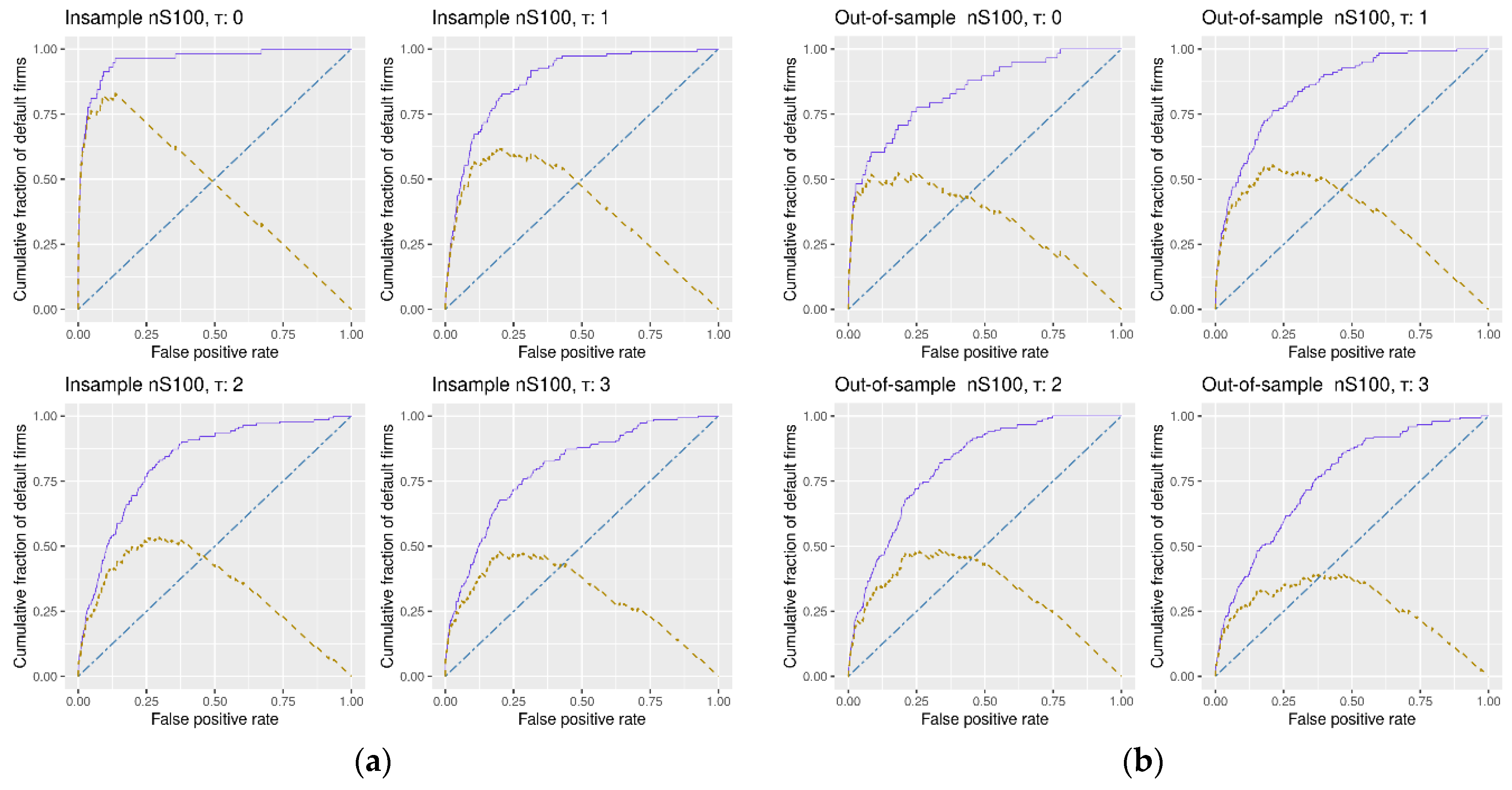
Our accuracy ratio is not the same as the area under curve, or AUC, also used in the literature. The latter amounts to 0.5 for a random classifier, an equivalent of the accuracy ratio of zero (see Table 3). Hence, the accuracy ratios of 0.8475, 0.8114, or 0.7590, that we record out-of-sample for tau = 1, tau = 2, and tau = 3, respectively, imply an AUC of 0.9238, 0.9057, and 0.8795, respectively. The difference between 0.7590 and 0.8795 in reported statistics is worth noting. The awareness of what measure is used to gauge the goodness-of-fit is important in any research. In the default literature, it is critical.

We also note the relatively low drop in the out-of-sample accuracy of 2–4 p.p., compared to the in-sample statistics. The finding is broadly in line with Duan et al. (2012). As illustrated by Table 17, the drop reported in Duan et al. (2012) is even smaller and amounts to merely one percentage point. As for the statistical inference, neither Duffie et al. (2007) nor Duan et al. (2012) deliver any statistical tests for the accuracy ratios. In contrast, our results are fully documented to be statistically significant at the 1% level using two different statistical tests.

In summary, we would like to reiterate the coherence and the robustness of the results obtained. Firstly, we note again that the signs of covariates, including those for critically important variables, are almost perfectly in line with the theoretical expectations. This is particularly rewarding, as we decided to represent every and each micro factor with two closely related ratios. We have verified this result by running an additional 100 different model specifications, e.g., with and without macro input, with micro variables represented by one or two ratios each, with or without the size control variable, etc. The signs stayed broadly unaffected. Secondly, the coefficient magnitudes confirm the time-dependent relationships. The closer to default, the greater the drop in liquidity and profitability, for example, resulting in ever higher default forward intensities. Thirdly, both in- and out-of-sample accuracy ratios are large and comparable in size with those generated for developed markets and public companies. Fourthly, the accuracy ratios monotonically change with time—the further away from default, the lower the power of the model discrimination. This is precisely what we expect. Fifthly, the accuracy of the model changes in line with the addition (or subtraction) of additional variables to the model. For example, scrapping the double representation of company-specific ratios results in the loss of accuracy ratios of around 3–4 percentage points. Aborting the macro factors cuts AR by another 4–5 percentage points. Finally, all of our replications result in both in- and out-of-sample results that are statistically significant at the 1% level, using two different tests. This all proves the model is far more resilient than traditionally used linear regression specifications to different model specification changes.

Last but not least, we reiterate that the doubly stochastic Poisson model used in this paper is still dependent, by definition, on the doubly stochastic assumption under which firms’ default times are correlated only in the way implied by the correlation of factors determining their default intensities. Notwithstanding our highly satisfactory and robust results, these results should be viewed with caution, as no doubt the model implies unrealistically low estimates of default correlations compared to the sample correlations. This has been reported by, for e.g., Das et al. (2007) and Duffie et al. (2000). It should also be remembered that the overlapped pseudo-likelihood function proposed by Duan et al. (2012) used in this paper does violate the standard assumptions, and the implications of this are not immediately clear. Still, the potential biases introduced affect the results of both Duffie et al. (2007) and/or Duan et al. (2012) as much they affect our findings.

5. Conclusions

The doubly stochastic Poisson process has proved to produce very robust default probabilities, not only for public firms operating in the high-quality reporting environment. In this paper, having conducted a meticulous data cross-check, we illustrated that the model is also capable of producing strong and reliable results for low-quality data on non-public firms from capital markets characterized by lower quality governance and transparency standards (Aluchna et al. 2019). Being assured of the model’s applicability, we must acknowledge that the wide range of unanswered questions, on top of those already mentioned in the Discussion section, still remains. Below, we present just a few of them in the form of an exemplary, less than complete, checklist, starting with the most obvious (based on the literature).

• We start with the most popular topic of default literature, i.e., the determinants of the default. What does exactly determine (describe) bankruptcy? In this paper, we selected some micro and macro factors without much attention attached to this issue. This is not to say it is unimportant. Quite the opposite. To know which company-specific attributes and macro influences add most to our understanding of forward default intensity is always rewarding.
• We acknowledge that Duan et al. (2012), via quite intricate, and sometimes quite arbitrary, in-house developed procedures, make all their input monthly. Given the practical importance of the timely reporting of default probabilities, the rationale for it is self-evident. We wonder how much this approach would affect our results in terms of both the goodness-of-fit and the robustness of our results.
• In order to capture the dynamics of the covariates, on top of the levels, Duan et al. (2012) introduce the first changes (called trends) in the values of state variables, too. Would that materially change our results?
• In this research, we identified default as a well-defined legal event within the context of Poland’s bankruptcy law (“the declaration of bankruptcy to liquidate the debtors’ assets”). Our decision was, to some extent, arbitrary, yet we acknowledge we have collected information on as many as 41 different legal events (starting from various court petitions, numerous different court decisions, to actual declarations of many types of bankruptcy proceedings). Would the model work for different types of “default definitions”? Would it discriminate successfully between event-positive and event-negative firms, regardless of the event definition?
• In defining survivors, we adopted a very strong criterion: no bankruptcy event of any sort during the sample period. No doubt, other, less restrictive rulings are also possible.
• Finally, we would like to emphasize the arbitrary nature of the match between the default event date and the date of the financial statement identified as the one that precedes the event—a typical issue in all default research. Simple lagging is an option. Yet, there are many other ways to do it, utilizing, for example, the information on actual filing timing. The timing of the filing may also be used as a proper signal itself (companies that file the accounts with a delay tend to be less financially reliable). The use of this information is certain to be particularly valuable in the context of non-public, low-quality players.

Given the nature of the data (which calls for many cross-checks and interpretations) and the novelty of the methodological approach, the list of various aspects worth researching is practically endless, ranging from detailed analysis of input data to searching for better estimators. Whatever the look of a complete list, it is comforting to know that compiling such a list makes sense in the first place, as we successfully demonstrated in this paper the applicability of the doubly stochastic formulation in the context of emerging market non-public firms producing low-quality inputs.

References

1. Acharya, Viral V., Matteo Crosignani, Tim Eisert, and Christian Eufinger. 2020. Zombie Credit and (Dis-)inflation: Evidence from Europe. National Bureau of Economic Research. Available online: https://www.nber.org/system/files/working_papers/w27158/w27158.pdf (accessed on 23 July 2021).
2. Altman, Edward I. 1968. Financial ratios, discriminant analysis and the prediction of corporate bankruptcy. The Journal of Finance 23: 589–609. [Google Scholar] [CrossRef]
3. Altman, Edward I. 2020. Covid-19 and the credit cycle. Journal of Credit Risk 16: 67–94. [Google Scholar]
4. Aluchna, Maria, Tomasz Berent, and Bogumił Kamiński. 2019. Dividend payouts and shareholder structure: Evidence from the Warsaw Stock Exchange. Eastern European Economics 57: 227–50. [Google Scholar] [CrossRef]
5. Banerjee, Ryan, and Boris Hofmann. 2018. The rise of zombie firms: Causes and consequences. BIS Quarterly Review September. pp. 67–78. Available online: https://www.bis.org/publ/qtrpdf/r_qt1809g.pdf (accessed on 20 October 2021).
6. Beaver, William H. 1966. Financial ratios as predictors of failure. Journal of Accounting Research 4: 71–111. [Google Scholar] [CrossRef]
7. Beaver, William H. 1968. Market prices, financial ratios, and the prediction of failure. Journal of Accounting Research 6: 179–92. [Google Scholar] [CrossRef]
8. Beaver, William H., Maureen F. McNichols, and Jung-Wu Rhie. 2005. Have financial statements become less informative? Evidence from the ability of financial ratios to predict bankruptcy. Review of Accounting Studies 10: 93–122. [Google Scholar] [CrossRef]
9. Berent, Tomasz, Bogusław Bławat, Marek Dietl, Przemysław Krzyk, and Radosław Rejman. 2017. Firm’s default? new methodological approach and preliminary evidence from Poland. Equilibrium. Quarterly Journal of Economics and Economic Policy 12: 753–73. [Google Scholar]
10. Bharath, Sreedhar T., and Tyler Shumway. 2008. Forecasting default with the Merton model. The Review of Financial Studies 21: 1339–69. [Google Scholar] [CrossRef]
11. Caporale, Guglielmo Maria, Mario Cerrato, and Xuan Zhang. 2017. Analysing the determinants of insolvency risk for general insurance firms in the UK. Journal of Banking & Finance 84: 107–22. [Google Scholar]
12. Chava, Sudheer, and Robert A. Jarrow. 2004. Bankruptcy prediction with industry effects. Review of Finance 8: 537–69. [Google Scholar] [CrossRef]
13. Collin-Dufresne, Pierre, and Robert S. Goldstein. 2001. Do credit spreads reflect stationary leverage ratios? The Journal of Finance 56: 1929–57. [Google Scholar] [CrossRef]
14. Das, Sanjiv R., Darrell Duffie, Nikunj Kapadia, and Leandro Saita. 2007. Common failings: How corporate defaults are correlated. The Journal of Finance 62: 93–118. [Google Scholar] [CrossRef]
15. DeLong, Elizabeth R., David M. DeLong, and Daniel L. Clarke-Pearson. 1988. Comparing the areas under two or more correlated receiver operating characteristic curves: A nonparametric approach. Biometrics 54: 837–45. [Google Scholar] [CrossRef]
16. Duan, Jin-Chuan, Jie Sun, and Tao Wang. 2012. Multiperiod corporate default prediction—A forward intensity approach. Journal of Econometric 170: 191–209. [Google Scholar] [CrossRef]
17. Duan, Jin-Chuan, Baeho Kim, Woojin Kim, and Donghwa Shin. 2018. Default probabilities of privately held firms. Journal of Banking & Finance 94: 235–50. [Google Scholar]
18. Duffie, Darrell, Andreas Eckner, Guillaume Horel, and Leandro Saita. 2000. Frailty Correlated Default. Journal of Finance 64: 2089–123. [Google Scholar] [CrossRef]
19. Duffie, Darrell, Leandro Saita, and Ke Wang. 2007. Multi-period corporate default prediction with stochastic covariates. Journal of Financial Economics 83: 635–65. [Google Scholar] [CrossRef] [Green Version]
20. Fischer, Edwin O., Robert Heinkel, and Josef Zechner. 1989. Dynamic capital structure choice: Theory and tests. The Journal of Finance 44: 19–40. [Google Scholar] [CrossRef]
21. Giesecke, Kay. 2004. Correlated default with incomplete information. Journal of Banking & Finance 28: 1521–45. [Google Scholar]
22. Hamilton, David T., and Richard Cantor. 2004. Rating transition and default rates conditioned on outlooks. The Journal of Fixed Income 14: 54–70. [Google Scholar] [CrossRef]
23. Hanley, James A., and Barbara J. McNeil. 1982. The meaning and use of the area under a receiver operating characteristic (ROC) curve. Radiology 143: 29–36. [Google Scholar] [CrossRef] [PubMed] [Green Version]
24. Hillegeist, Stephen A., Elizabeth K. Keating, Donald P. Cram, and Kyle G. Lundstedt. 2004. Assessing the probability of bankruptcy. Review of Accounting Studies 9: 5–34. [Google Scholar] [CrossRef]
25. Jarrow, Robert A., and Fan Yu. 2001. Counterparty risk and the pricing of defaultable securities. The Journal of Finance 56: 1765–99. [Google Scholar] [CrossRef]
26. Kalbfleisch, John D., and Ross Prentice. 2002. The Statistical Analysis of Failure Time Data, 2nd ed. Hoboken: Wiley. [Google Scholar]
27. Kavvathas, Dimitrios. 2000. Estimating Credit Rating Transition Probabilities for Corporate Bonds. AFA 2001 New Orleans Meetings. Available online: https://ssrn.com/abstract=252517 (accessed on 23 July 2021).
28. Lancaster, Tom. 1990. The Econometric Analysis of Transition Data. Cambridge: Cambridge University Press. [Google Scholar]
29. Leland, Hayne E. 1994. Corporate debt value, bond covenants, and optimal capital structure. The Journal of Finance 49: 1213–52. [Google Scholar] [CrossRef]
30. Merton, Robert C. 1974. On the pricing of corporate debt: The risk structure of interest rates. The Journal of Finance 29: 449–70. [Google Scholar]
31. Ohlson, James A. 1980. Financial ratios and the probabilistic prediction of bankruptcy. Journal of Accounting Research 18: 109–31. [Google Scholar] [CrossRef] [Green Version]
32. Schoenbucher, Philipp. 2003. Information-driven default contagion. Department of Mathematics, ETH Zurich. Available online: http://citeseerx.ist.psu.edu/viewdoc/download?doi=10.1.1.139.2714&rep=rep1&type=pdf (accessed on 23 July 2021).
33. Shumway, Tyler. 2001. Forecasting bankruptcy more accurately: A simple hazard model. The Journal of Business 74: 101–24. [Google Scholar] [CrossRef] [Green Version]
34. Zmijewski, Mark E. 1984. Methodological issues related to the estimation of financial distress prediction models. Journal of Accounting Research 25: 59–82. [Google Scholar] [CrossRef]
Figure 1. The number of liquidation proceedings vs. restructuring proceedings in Poland (pre-2016 restructuring proceedings not recorded) (Polish Institute of Credit Management).
Risks 09 00217 g001
Figure 2. The number of company-years from 2007 to 2017.
Risks 09 00217 g002
Figure 3. The number of companies declared bankrupt between 2011 and 2018.
Risks 09 00217 g003
Figure 4. Cash to total asset: (a) default companies; (b) survivors vs. default companies three years before default.
Risks 09 00217 g004
Figure 5. Current assets to current liabilities: (a) default companies; (b) survivors vs. default companies three years before default.
Risks 09 00217 g005
Figure 6. Net profit to total assets: (a) default companies; (b) survivors vs. default companies three years before default.
Risks 09 00217 g006
Figure 7. EBIT margin: (a) default companies; (b) survivors vs. default companies three years before default.
Risks 09 00217 g007
Figure 8. Net debt to equity: (a) default companies; (b) survivors vs. default companies three years before default.
Risks 09 00217 g008
Figure 9. Net debt to EBIT: (a) default companies; (b) survivors vs. default companies three years before default.
Risks 09 00217 g009
Figure 10. Total assets rotation: (a) default companies; (b) survivors vs. default companies three years before default.
Risks 09 00217 g010
Figure 11. Short-term receivables rotation: (a) default companies; (b) survivors vs. default companies three years before default.
Risks 09 00217 g011
Figure 12. Revenue: (a) default companies; (b) survivors vs. default companies three years before default.
Risks 09 00217 g012
Figure 13. Total assets: (a) default companies; (b) survivors vs. default companies three years before default.
Risks 09 00217 g013
Figure 14. ROC curves for tau = 1, tau = 2, tau = 3 (tau = 0 for comparison only): (a) in-sample; (b) out-of-sample.
Risks 09 00217 g014