Stochastic Claims Reserving Methods with State Space Representations: A Review

Abstract

Often, the claims reserves exceed the available equity of non-life insurance companies and a change in the claims reserves by a small percentage has a large impact on the annual accounts. Therefore, it is of vital importance for any non-life insurer to handle claims reserving appropriately. Although claims data are time series data, the majority of the proposed (stochastic) claims reserving methods is not based on time series models. Among the time series models, state space models combined with Kalman filter learning algorithms have proven to be very advantageous as they provide high flexibility in modeling and an accurate detection of the temporal dynamics of a system. Against this backdrop, this paper aims to provide a comprehensive review of stochastic claims reserving methods that have been developed and analyzed in the context of state space representations. For this purpose, relevant articles are collected and categorized, and the contents are explained in detail and subjected to a conceptual comparison.

1. Introduction

1.1. The Importance of Claims Reserving in Non-Life Insurance

The insurance industry offers a multi-faceted range of numerous products that enable policyholders to insure themselves against almost any form of loss. Insurance companies therefore differentiate their products according to various criteria. In this paper, we focus on the problem of claims reserving for a branch of insurance products known as Non-Life Insurance (Continental Europe), General Insurance (United Kingdom) and Property and Casualty Insurance (USA). While this branch encompasses all insurance products that are different from life insurance, life insurance includes only life-related products and disability insurance (see Wüthrich and Merz 2008). This is due to the following reasons. On the one hand, life and non-life products differ reasonably, which is mainly reflected in the contract terms, types of claims and risk drivers. This also explains why different stochastic models and methods are used in both these branches. On the other hand, in many countries (such as Germany or Switzerland), there is a strict legal separation between life and non-life. A non-life insurer is therefore prohibited from offering life products, and vice versa. For this reason, it is not uncommon for insurance corporations to establish different companies and thus sell products from both branches. The following lines of business belong to the non-life insurance branch: motor/car insurance, property insurance, liability insurance, accident insurance, health insurance, marine insurance, and other insurance products such as aviation, credit insurance, epidemic insurance, legal protection, travel insurance, and so on (see Wüthrich and Merz 2008).

The amount of money that a policyholder has to pay to the insurer for insurance coverage is called the premium. By paying a premium, the policyholder under an insurance policy transfers the risk to the insurer (risk transfer), who has to compensate/settle the potential loss occurring under the contract via corresponding claims payments (in whole or in part). This practice represents the insurance principle of non-life insurance. Thus, in contrast to life insurance, non-life insurance is loss insurance, i.e., payments are made by the insurer to the policyholder only in the event of a specific loss.

At the end of each fiscal year, the insurer is confronted with the situation in which the premiums are known, but the claim amount is unknown. This uncertainty of the total loss liabilities is mainly due to (1) a reporting delay, (2) a long-lasting claim settlement, and (3) the unexpected re-opening of a closed claim (see Wüthrich and Merz 2008). Therefore, appropriate claims reserves for the outstanding loss liabilities have to be calculated by the responsible actuary. Since these loss reserves are often the largest share on the liability side of the balance sheet, adequate claims reserving is required, that is, forecasting these liabilities and quantifying their uncertainty is a key actuarial issue (see Chukhrova and Johannssen 2021).

Although claims data are time series data, the majority of the proposed (stochastic) claims reserving methods is not based on time series models. Among the time series models, state space models combined with Kalman filter learning algorithms have proven to be very advantageous as they provide high flexibility in modeling and an accurate detection of the temporal dynamics of a system (see Chukhrova and Johannssen 2021). Against this backdrop, this paper aims to provide a comprehensive review of stochastic claims reserving methods that have been developed and analyzed in the context of state space representations. For this purpose, relevant articles are collected and categorized, the contents are explained in detail and subjected to a conceptual comparison.

1.2. State Space Models in the Claims Reserving Literature

The actuarial literature contains various articles in which state space models and the Kalman filter learning algorithms are applied to improve stochastic claims reserving (see Johannssen 2016). As a pioneer, De Jong and Zehnwirth (1983) constructed a state space model for the payment stream of incremental payments, took business volume and inflation indices into account, and presented a method to estimate the states underlying the observations of the upper triangle and to predict the outstanding loss liabilities of the lower triangle. Afterwards, Verrall (1989) used the relationship between the two-way ANOVA and the Chain Ladder (CL) method to establish a state space model for the so-called linear CL model. Wright (1990) constructed a model for incremental payments and employed the state space approach to model variations in parameters across different accident years. Verrall (1994) extended the state space model of Verrall (1989) to weaken the homogeneity property of the CL method, which allows for development factors that do not necessarily have to be identical across all accident years. Zehnwirth (1997) considered different recursive representations, including state space models based on the general form introduced by De Jong and Zehnwirth (1983) and discussed calendar year effects in claims development triangles.

Ntzoufras and Dellaportas (2002) presented four models for Reported But Not Settled (RBNS) claims, including state space models following Verrall (1989, and 1994). Alpuim and Ribeiro (2003) proposed a univariate distribution-free state space model, where incremental payments are modeled as a function of payments of the first development year, i.e., the accident year itself. Taylor et al. (2003) discussed a generalized Kalman filter that accounts for non-linearities in the observation equation. De Jong (2005) considered the so-called development correlation model, which is a (state space) model that accounts for correlations between individual development factors in the first two development years. In addition, De Jong (2006) not only discussed the development correlation model, but two further approaches taking correlations related to accident and calendar years into account.

Li (2006) compared various claims reserving methods including the state space model of Verrall (1989). A completely different approach from the previous articles is taken by Atherino et al. (2010), who did not model the Incurred But Not Reported (IBNR) run-off data in chronological form, but as a univariate time series with missing observations. Pang and He (2012) combined the approach of Verrall (1989) and Taylor et al. (2003) and included an additional lag of the state vector into the state equation. Chukhrova and Johannssen (2017) presented a scalar state space model for cumulative payments. Most recently, Costa and Pizzinga (2020) and Hendrych and Cipra (2021) extended the row-wise stacking approach from Atherino et al. (2010) through the inclusion of tail effects and multivariate considerations that allow for dependency modeling between correlated lines of business, respectively.

1.3. Categorization of Articles and Organization of the Paper

Figure 1 shows the history of the considered articles in stochastic claims reserving. Thereby, all articles are ordered chronologically and are classified into five categories considering their similarities in terms of contents: “Parametric evolution”, “Log-normal model”, “Correlation models”, “Univariate models”, and “Row-wise stacking”. These categories need not be taken as mutually exclusive, but the choice of the appropriate category is made considering the main approach used in the respective paper. The first category includes the articles by De Jong and Zehnwirth (1983), Wright (1990), Zehnwirth (1997), Taylor et al. (2003), and Pang and He (2012), as they are based on the assumption of a parametric evolution of the run-off data across the development years. The second category includes the articles by Verrall (1989, 1994), Ntzoufras and Dellaportas (2002), Li (2006) because of the considered log-normal model for incremental payments. The third category consists of the articles by De Jong (2005, and 2006) who discusses three types of models that incorporate correlations within claims development triangles. In the fourth category, there are the articles by Alpuim and Ribeiro (2003) and Chukhrova and Johannssen (2017), where models are presented that avoid complex matrix-based structures. Finally, the fifth category include the articles by Atherino et al. (2010), Costa and Pizzinga (2020), and Hendrych and Cipra (2021), who propose a row-wise stacking of the claims data and associated state space representations. The solid arrows in Figure 1 represent the contentual similarities among the papers in their modeling approaches. The dashed arrows indicate, however, that the respective state space models are included in papers where different stochastic claims reserving methods are compared (see England and Verrall 2002; Verrall 2004). In addition, state space models and the Kalman learning algorithms are discussed in the context of stochastic claims reserving in standard text books such as Wüthrich and Merz (2008).

Figure 1. Chronology and categorization of the papers.

In the following, a category-guided presentation of the articles is performed. Within each of five categories, a chronological order is followed to present the individual articles. For the sake of consistency, a unified notation is used throughout the paper. Since this paper is devoted to state space representations, all essential contents concerning state space models are presented in the following, whereas less relevant contents are omitted or referred to. In particular, the state space representations given in the articles are developed in full detail, often much more detailed than in the original papers.

The paper is organized as follows. In Section 2, articles are discussed that are based on the assumption of a parametric evolution of the claims data across development years (Category 1). Section 3 presents articles in which incremental payments are assumed to be log-normally distributed and are modeled using a log-normal model (Category 2). Section 4 includes articles where correlation models are considered (Category 3). In Section 5, state space models are presented that have a scalar structure (Category 4). Section 6 contains articles where the row-wise stacking approach is considered to re-organize the claims data (Category 5). Subsequently, Section 7 provides a conceptual comparison of the presented approaches and state space representations. In Section 8, concluding remarks are given.

2. Parametric Evolution of Claims Data (Category 1)

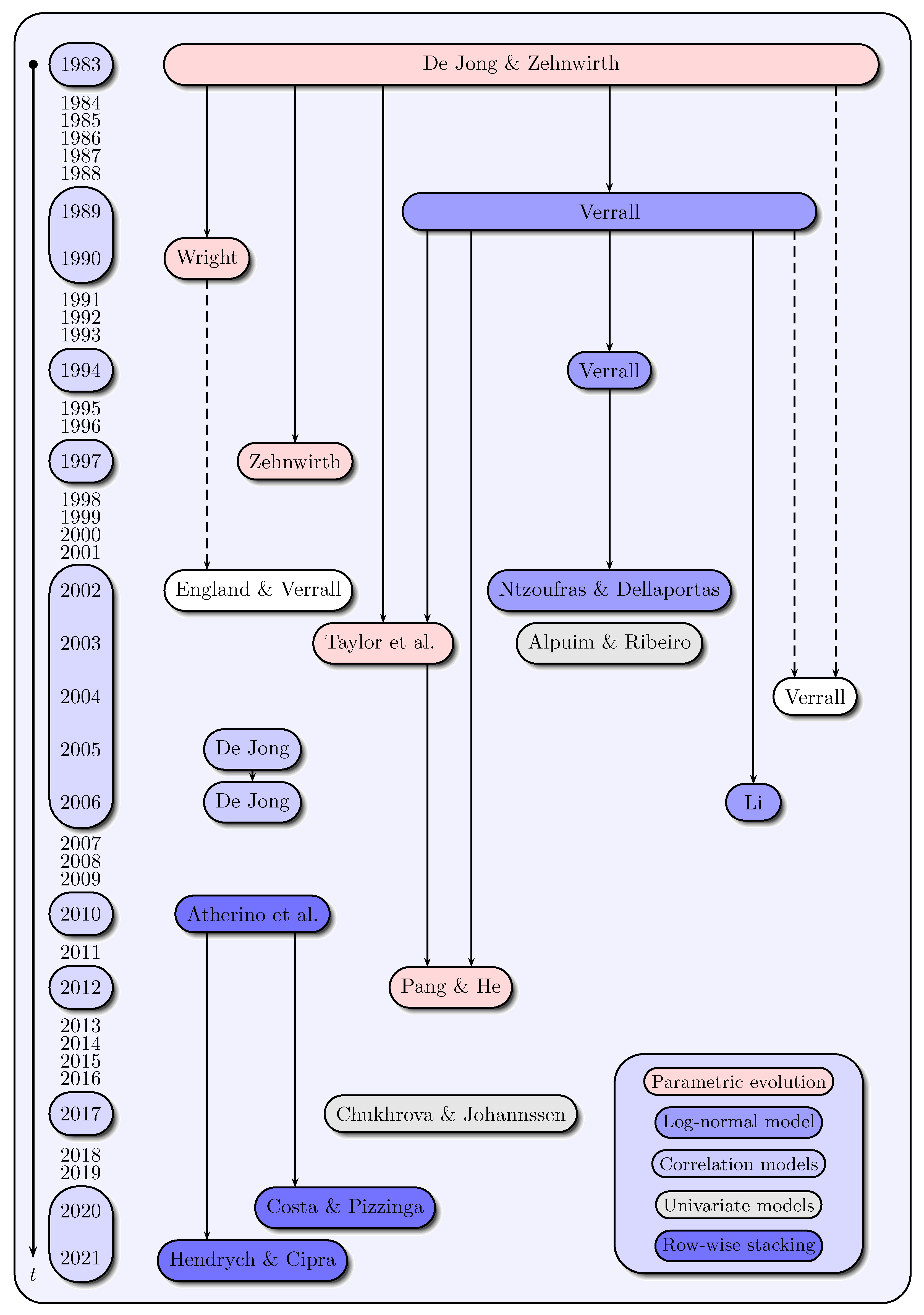
In this section, we present papers that are based on the assumption of a parametric evolution of the claims data across development years:

▸

De Jong and Zehnwirth (1983): Claims Reserving, State-Space Models and the Kalman Filter;

⊳

Wright (1990): A Stochastic Method for Claims Reserving in General Insurance;

⊳

Zehnwirth (1997): Kalman Filters with Applications to Loss Reserving;

▸

Taylor et al. (2003): Loss Reserving: Past, Present and Future;

▸

Pang and He (2012): Application of State Space Model in Outstanding Claims Reserve.

Three articles marked with ▸ are mainly based on the use of state space models and the Kalman filter learning theory, and thus are presented in detail, while the models of the other two articles marked with ⊳ are treated in a more brief form, as state space models are not the focus of their methodologies.

2.1. Claims Reserving, State Space Models and the Kalman Filter

De Jong and Zehnwirth (1983) laid the foundation for the use of state space models and the Kalman filter in stochastic claims reserving with their article “Claims Reserving, State-Space Models and the Kalman Filter”. The proposed state space model is constructed for the payment stream of the incremental payments and presumes known, time-varying system matrices.

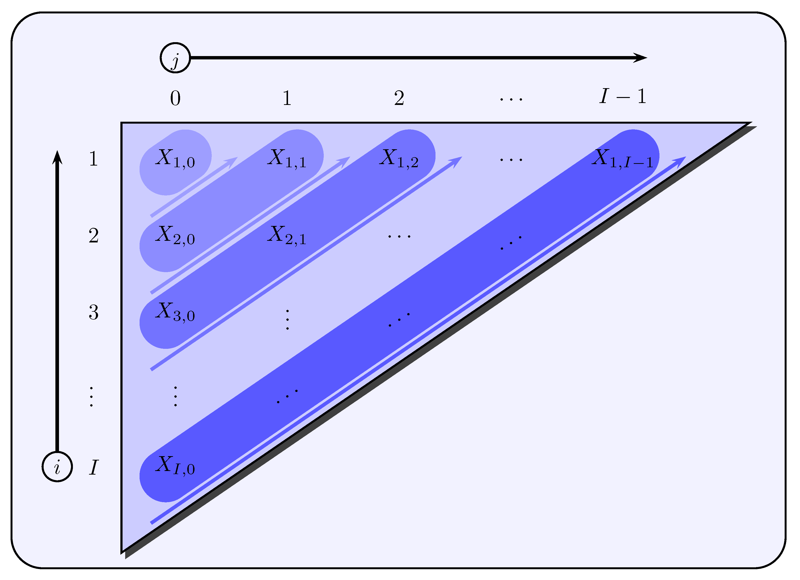
$⊳$ Modeling the payment stream of incremental payments

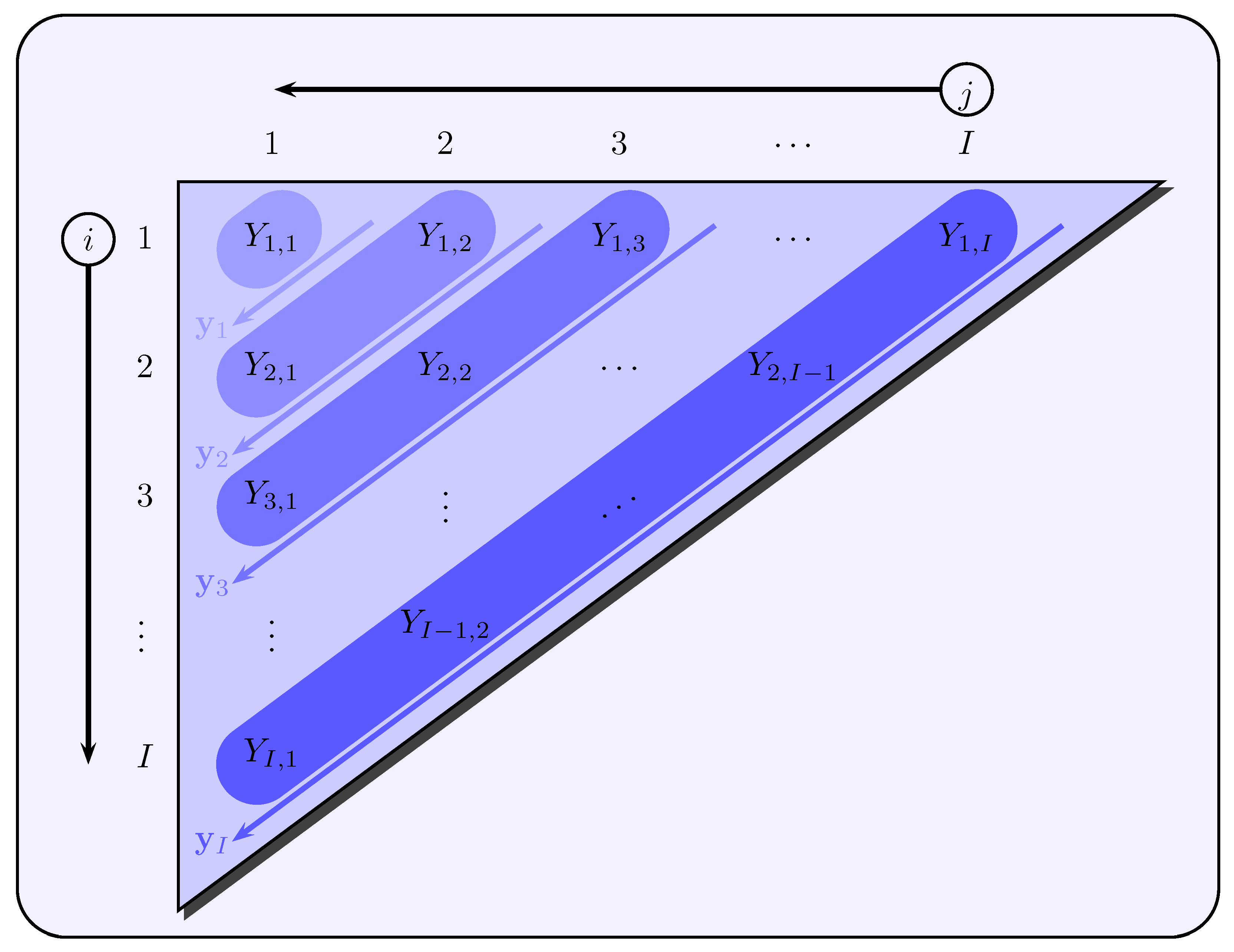
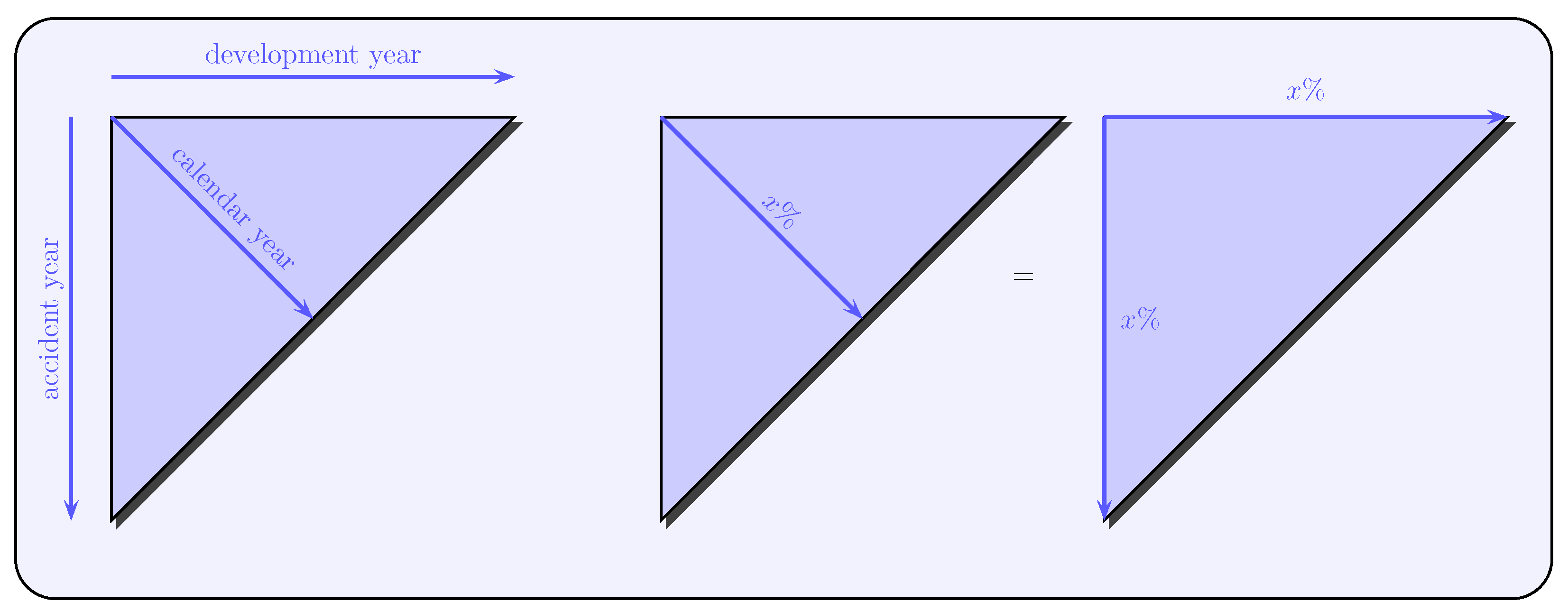
The modeling is based on claims development triangles in which incremental payments $X_{i,j}$ are given for accident years $i=1,\dots ,I$ and development years $j=0,\dots ,I-1$. The payment stream of incremental payments is modeled with increasing development year $j=0,\dots ,t-1$ and decreasing accident year $i=t,t-1,\dots ,1$ for a fixed calendar year $t=i+j$ via

$$\begin{array}{c}\hfill X_{i,j}=m(t-j,j)+u_j\left(t\right),\end{array}$$

(1)

see also Figure 2. Here, the quantity $m(t-j,j)=m(i,j)$ is generally the expected claim payment to be made in accident year i and development year j of the t-th calendar year, and $u_j\left(t\right)$ is a noise term with $\mathbb{E}\left[u_j\left(t\right)\right]=0$.

Figure 2. Modeling the payment stream of incremental payments.

De Jong and Zehnwirth (1983) propose an optional modification of (1) by including additional information such as the volume of business transacted in each accident year and the inflation factor for each calendar year. To this end, let $n\left(i\right)$ denote an appropriate index for the volume of business transacted in accident year i and $\lambda \left(t\right)$ denote an appropriate price index for payments in the t-th calendar year. Using both these quantities, (1) can be extended to

$$\begin{array}{c}\hfill X_{i,j}=n(t-j)\lambda \left(t\right)m(t-j,j)+u_j\left(t\right),\end{array}$$

(2)

where $n(t-j)\lambda \left(t\right)m(t-j,j)$ is the expected value of the inflation-adjusted and volume-weighted incremental payments in accident year i and development year j of calendar year t.

$⊳$ Development of an appropriate state space representation

The modeling of the payment stream via (1) and (2) is promising with respect to the construction of an appropriate observation and state equation of a state space model, respectively. The following discussion in this regard is based on (1), but can be applied to (2) with minor modifications. In the first step of modeling the observation equation, (1) is transferred into a vector representation in such a way that ${\mathbf{y}}_t$ represents the vector of observations $X_{i,j}$ of the t-th calendar year, ${\mathbf{f}}_t$ forms the vector of expected claims payments $m(t-j,j)$, and ${\mathbf{w}}_t$ is the vector of noise terms $u_j\left(t\right)$ with $j=0,\dots ,t-1$. Thus, the incremental payments made in calendar year t can be specified via

$$\begin{array}{c}\hfill \left(\begin{array}{c}{X}_{t,0}\\ X_{t-1,1}\\ ⋮\\ X_{1,t-1}\end{array}\right)=\left(\begin{array}{c}m(t,0)\\ m(t-1,1)\\ ⋮\\ m(1,t-1)\end{array}\right)+\left(\begin{array}{c}{u}_0\left(t\right)\\ u_1\left(t\right)\\ ⋮\\ u_{t-1}\left(t\right)\end{array}\right)\end{array}$$

(3)

or briefly as ${\mathbf{y}}_t={\mathbf{f}}_t+{\mathbf{w}}_t$. In the second step, the vector ${\mathbf{f}}_t$ is to be modeled in such a way that it is obtained by the product of a system matrix ${\mathbf{G}}_t$ and a state vector ${\mathbf{x}}_t$. For this purpose, De Jong and Zehnwirth (1983) take $m(i,j)$ for a given accident year i as a function depending on the development year j and thus construct for each accident year a distributed lag model of the form

$$\begin{array}{c}\hfill m(i,j)=\sum _{k=1}^p{\varphi }_k\left(j\right)b_k\left(i\right),\end{array}$$

(4)

where ${\varphi }_k\left(j\right)$ are known functions in j and $b_k\left(i\right)$ are unknown parameters depending on the respective accident year i. De Jong and Zehnwirth (1983) justified the approach (4) by an overall smooth evolution of $m(i,j)$ characterized by a firstly increasing and then decreasing behavior in j for a given accident year i. A variation of (4) for $p=1$ is the so-called Hoerl curve

$$\begin{array}{c}\hfill m(i,j)=b\left(i\right)(j+1)e^{-j},\end{array}$$

(5)

which De Jong and Zehnwirth (1983) use in their empirical application example. In addition, (4) can be easily transferred into vector notation by using

$$\begin{array}{c}\hfill \mathbf{\varphi }\left(j\right)=\left(\begin{array}{c}{\varphi }_1\left(j\right)\\ {\varphi }_2\left(j\right)\\ ⋮\\ {\varphi }_p\left(j\right)\end{array}\right)\mathrm{and}\mathbf{b}\left(i\right)=\left(\begin{array}{c}{b}_1\left(i\right)\\ b_2\left(i\right)\\ ⋮\\ b_p\left(i\right)\end{array}\right)\end{array}$$

(6)

as follows:

$$\begin{array}{c}\hfill m(i,j)={\mathbf{\varphi }}^T\left(j\right)\mathbf{b}\left(i\right)\end{array}$$

(7)

Substituting (7) into (3) then gives

$$\begin{array}{cc}\left(\begin{array}{c}{X}_{t,0}\\ X_{t-1,1}\\ ⋮\\ X_{1,t-1}\end{array}\right)\hfill & =\left(\begin{array}{c}{\mathbf{\varphi }}^T\left(0\right)\mathbf{b}\left(t\right)\\ {\mathbf{\varphi }}^T\left(1\right)\mathbf{b}(t-1)\\ ⋮\\ {\mathbf{\varphi }}^T(t-1)\mathbf{b}\left(1\right)\end{array}\right)+\left(\begin{array}{c}{u}_0\left(t\right)\\ u_1\left(t\right)\\ ⋮\\ u_{t-1}\left(t\right)\end{array}\right)\hfill \\ \hfill & =\left(\begin{array}{cccc}{\mathbf{\varphi }}^T\left(0\right)& {\mathbf{0}}^T& \dots & {\mathbf{0}}^T\\ {\mathbf{0}}^T& {\mathbf{\varphi }}^T\left(1\right)& & ⋮\\ ⋮& & \ddots & {\mathbf{0}}^T\\ {\mathbf{0}}^T& \dots & {\mathbf{0}}^T& {\mathbf{\varphi }}^T(t-1)\end{array}\right)\left(\begin{array}{c}\mathbf{b}\left(t\right)\\ \mathbf{b}(t-1)\\ ⋮\\ \mathbf{b}\left(1\right)\end{array}\right)+\left(\begin{array}{c}{u}_0\left(t\right)\\ u_1\left(t\right)\\ ⋮\\ u_{t-1}\left(t\right)\end{array}\right)\hfill \end{array}$$

(8)

or in a more compact form

$$\begin{array}{c}\hfill {\mathbf{y}}_t={\mathbf{G}}_t{\mathbf{x}}_t+{\mathbf{w}}_t(\mathrm{observation}\mathrm{equation})\end{array}$$

(9)

with $\mathbb{E}\left[{\mathbf{w}}_t\right]=\mathbf{0}$ and

$$\begin{array}{c}\hfill \mathbb{E}\left[{\mathbf{w}}_s{\mathbf{w}}_t^T\right]=\left\{\begin{array}{cc}{\mathbf{R}}_t\hfill & \mathrm{i}\mathrm{f}s=t\hfill \\ \mathbf{O}\hfill & \mathrm{o}\mathrm{t}\mathrm{h}\mathrm{e}\mathrm{r}\mathrm{w}\mathrm{i}\mathrm{s}\mathrm{e}\hfill \end{array}\right.\end{array}$$

for all $s,t=1,\dots ,I$. Thus, given $\mathbf{\varphi }\left(j\right)$, $j=0,\dots ,t-1$, the system matrix ${\mathbf{G}}_t$ is a known time-varying diagonal matrix, and the state vector ${\mathbf{x}}_t$ contains unknown parameter vectors $\mathbf{b}\left(i\right)$ for $i=1,\dots ,t$. Assuming a Hoerl curve according to (5), the observation Equation (9) of the t-th calendar year results in (due to $p=1$):

$$\begin{array}{cc}\hfill \left(\begin{array}{c}{X}_{t,0}\\ X_{t-1,1}\\ ⋮\\ X_{1,t-1}\end{array}\right)& =\left(\begin{array}{cccc}1& 0& \dots & 0\\ 0& 2e^{-1}& & ⋮\\ ⋮& & \ddots & ⋮\\ 0& \dots & 0& t{e}^{1-t}\end{array}\right)\left(\begin{array}{c}b\left(t\right)\\ b(t-1)\\ ⋮\\ b\left(1\right)\end{array}\right)+\left(\begin{array}{c}{u}_0\left(t\right)\\ u_1\left(t\right)\\ ⋮\\ u_{t-1}\left(t\right)\end{array}\right)\hfill \end{array}$$

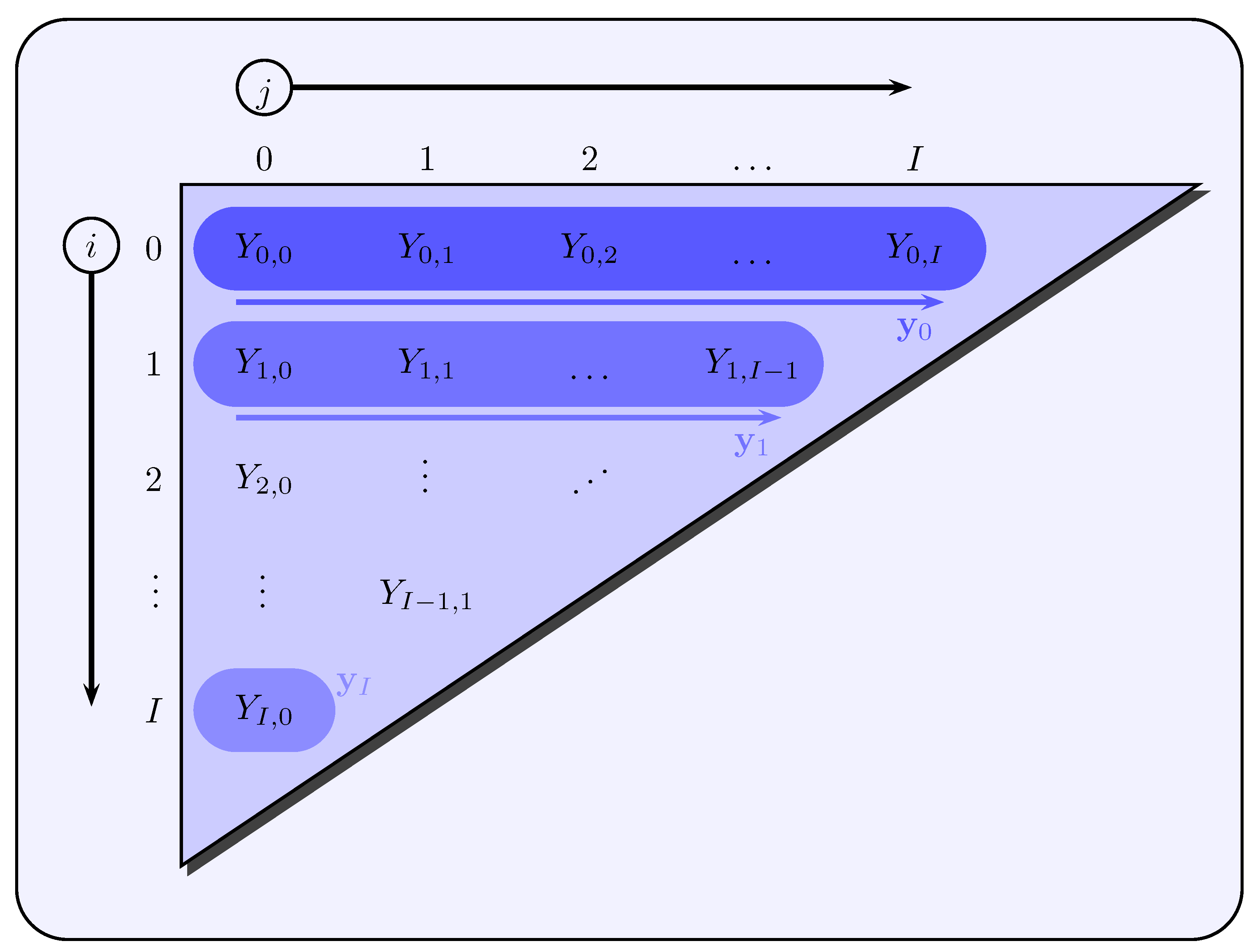
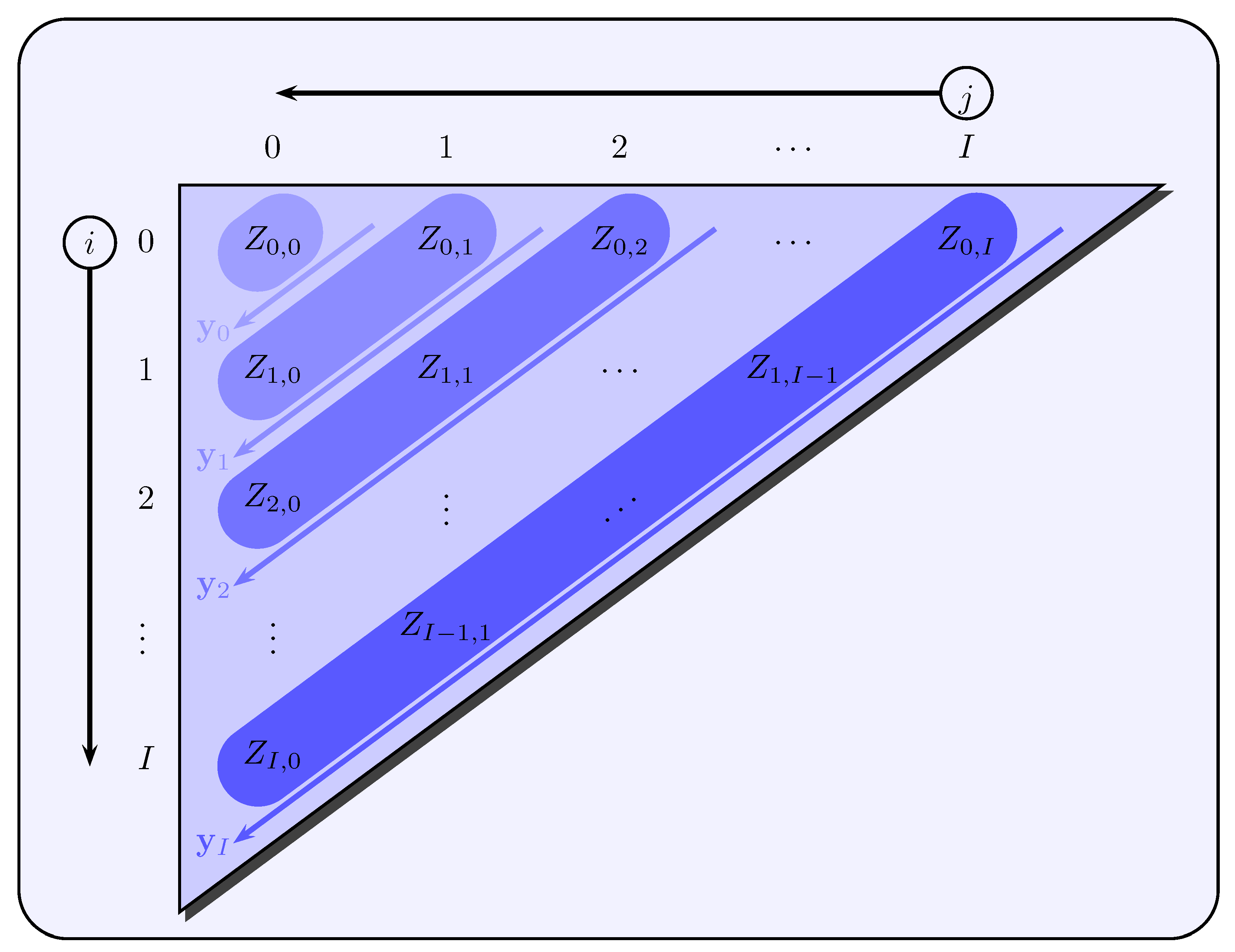
Subsequently, De Jong and Zehnwirth (1983) specify an appropriate state equation, in which they establish a connection between the state vector ${\mathbf{x}}_t$ of the t-th calendar year and the state vector ${\mathbf{x}}_{t-1}$ of the $(t-1)$-th calendar year. The basic idea is again to model a smooth evolution, but in a slightly different form than in (4). The starting point is the sequence $m(i,j)$, but with the difference that for a fixed development year j the accident years i are varied, whereas before for a fixed calendar year t the development years j varied (see Figure 3).

Figure 3. Sequences $m(i,j)$ for a given development year j.

For a given development year j, De Jong and Zehnwirth (1983) propose modeling $m(i,j)$ via

$$\begin{array}{c}\hfill m(i,j)=\mathbb{E}\left[m\right(i,j\left)\right|m(i-1,j),\dots ,m(i-q,j)]+\eta (i,j)\end{array}$$

(10)

with $q=1,\dots ,i-1$, where $\eta (i,j)$ is a noise term with $\mathbb{E}\left[\eta \right(i,j\left)\right]=0$. Thus, in contrast to (4), $m(i,j)$ is not modeled in a deterministic way but as a random variable. Further, they assume that the conditional expected value on the right-hand side of (10) is a polynomial in i of degree $q-1$ that passes through $m(i-1,j),\dots ,m(i-q,j)$. This leads to

$$\begin{array}{c}\hfill m(i,j)=\sum _{k=1}^{q}a\left(k\right)m(i-k,j)+\eta (i,j)\end{array}$$

(11)

with known

$$\begin{array}{c}\hfill a\left(k\right)=\left(\genfrac{}{}{0pt}{}{q}{k}\right){(-1)}^{k-1}\end{array}$$

for $k=1,\dots ,q$. Substituting (7) on both sides into (11) for $j=j_1,j_2,\dots ,j_p$ yields

$$\begin{array}{c}\hfill \mathsf{\Phi }\mathbf{b}\left(i\right)=\sum _{k=1}^{q}a\left(k\right)\mathsf{\Phi }\mathbf{b}(i-k)+{\mathbf{v}}_i,\end{array}$$

(12)

where the ($p\times p$)-dimensional matrix $\mathsf{\Phi }$ and the p-dimensional vector ${\mathbf{v}}_i$ are given by

$$\begin{array}{c}\hfill \mathsf{\Phi }=\left(\begin{array}{c}{\mathbf{\varphi }}^T\left(j_1\right)\\ {\mathbf{\varphi }}^T\left(j_2\right)\\ ⋮\\ {\mathbf{\varphi }}^T\left(j_p\right)\end{array}\right)\mathrm{and}{\mathbf{v}}_i=\left(\begin{array}{c}\eta (i,j_1)\\ \eta (i,j_2)\\ ⋮\\ \eta (i,j_p)\end{array}\right),\end{array}$$

respectively. If both sides of Equation (12) are multiplied from the left by the inverse ${\mathsf{\Phi }}^{-1}=\mathsf{\Psi }$ of the matrix $\mathsf{\Phi }$ (the existence of the inverse is ensured, see De Jong and Zehnwirth 1983), one obtains

$$\begin{array}{c}\hfill \mathbf{b}\left(i\right)=\sum _{k=1}^{q}a\left(k\right)\mathbf{b}(i-k)+\mathsf{\Psi }{\mathbf{v}}_i.\end{array}$$

(13)

Transferring (13) into matrix notation, we obtain

$$\begin{array}{c}\hfill \left(\begin{array}{c}\mathbf{b}\left(t\right)\\ \mathbf{b}(t-1)\\ ⋮\\ \mathbf{b}\left(1\right)\end{array}\right)=\left(\begin{array}{ccccc}a\left(1\right)\mathbf{I}& \dots & a\left(q\right)\mathbf{I}& \dots & \mathbf{O}\\ \mathbf{I}& \dots & \mathbf{O}& \dots & \mathbf{O}\\ ⋮& \ddots & ⋮& & ⋮\\ \mathbf{O}& & \mathbf{I}& & \mathbf{O}\\ ⋮& & ⋮& \ddots & ⋮\\ \mathbf{O}& \dots & \mathbf{O}& \dots & \mathbf{I}\end{array}\right)\left(\begin{array}{c}\mathbf{b}(t-1)\\ ⋮\\ \mathbf{b}(t-q)\\ ⋮\\ \mathbf{b}\left(1\right)\end{array}\right)+\left(\begin{array}{c}\mathsf{\Psi }\\ \mathbf{O}\\ ⋮\\ \mathbf{O}\end{array}\right){\mathbf{v}}_t\end{array}$$

(14)

or in a more compact fom

$$\begin{array}{c}\hfill {\mathbf{x}}_t={\mathbf{F}}_t{\mathbf{x}}_{t-1}+{\mathbf{B}}_t{\mathbf{v}}_t(\mathrm{state}\mathrm{equation})\end{array}$$

(15)

with $\mathbb{E}\left[{\mathbf{v}}_t\right]=\mathbf{0}$ and

$$\begin{array}{c}\hfill \mathbb{E}\left[{\mathbf{v}}_s{\mathbf{v}}_t^T\right]=\left\{\begin{array}{cc}{\mathbf{Q}}_t\hfill & \mathrm{i}\mathrm{f}s=t\hfill \\ \mathbf{O}\hfill & \mathrm{o}\mathrm{t}\mathrm{h}\mathrm{e}\mathrm{r}\mathrm{w}\mathrm{i}\mathrm{s}\mathrm{e}\hfill \end{array}\right.\end{array}$$

as well as $\mathbb{E}\left[{\mathbf{v}}_s{\mathbf{w}}_t^T\right]=\mathbf{O}$ for all $s,t=1,\dots ,I$. The identity matrices $\mathbf{I}$, zero matrices $\mathbf{O}$ and scalar matrices $a\left(k\right)\mathbf{I}$ with $k=1,\dots ,q$ in (14) are each of dimension $p\times p$. Note also that the system matrices ${\mathbf{F}}_t$ and ${\mathbf{B}}_t$ are known in the state Equation (15).

A variation of the state Equation (15) is given for $p=1$ (i.e., assuming a Hoerl curve as in (5)) and the parameters $b\left(i\right)$ of different accident years $i=2,\dots ,I$ are connected by a random walk

$$\begin{array}{c}\hfill b\left(i\right)=b(i-1)+v_i,\end{array}$$

(16)

that is, $q=1$, $a\left(1\right)=1$, $\mathsf{\Psi }=1$. Since we have $\mathsf{\Phi }={\mathbf{\varphi }}^T\left(j\right)=\mathbf{\varphi }\left(j\right)=(j+1)e^{-j}$, the relation $\mathsf{\Psi }=\frac{e^j}{j+1}$ holds. For this reason, De Jong and Zehnwirth (1983) aim to obtain $\mathsf{\Psi }=1$ and thus a state equation in the form of the random walk (16), i.e., they choose without loss of generality the fixed development year $j=0$.

With respect to (10) and (13), the use of (16) implies

$$\begin{array}{c}\hfill \mathbb{E}\left[m\right(i,j\left)\right|m(i-1,j),\dots ,m(i-q,j)]=\mathbb{E}[m(i,j)\left|m\right(i-1,j\left)\right]=m(i-1,j)\end{array}$$

for all $j=0,\dots ,I-1$. Accordingly, it follows for the system matrix ${\mathbf{F}}_t$ that it has the value one at positions $(1,1),(2,1),(3,2),\dots ,(t,t-1)$ and zeros otherwise, while ${\mathbf{B}}_t$ corresponds to a t-dimensional unit vector with the value one at position $(1,1)$. The state Equation (15) thus simplifies to:

$$\begin{array}{cc}\hfill \left(\begin{array}{c}b\left(t\right)\\ b(t-1)\\ ⋮\\ b\left(1\right)\end{array}\right)& =\left(\begin{array}{cccc}1& 0& \dots & 0\\ 1& 0& \dots & 0\\ ⋮& \ddots & & ⋮\\ ⋮& & 1& 0\\ 0& \dots & 0& 1\end{array}\right)\left(\begin{array}{c}b(t-1)\\ b(t-2)\\ ⋮\\ b\left(1\right)\end{array}\right)+\left(\begin{array}{c}1\\ 0\\ ⋮\\ 0\end{array}\right)v_t\hfill \end{array}$$

Table 1 gives an overview of the dimensions of vectors and matrices in the state space model of De Jong and Zehnwirth (1983).

Table 1. Dimensions in the state space model of De Jong and Zehnwirth (1983).

Vectors		Matrices
${\mathbf{y}}_t$	$t\times 1$	${\mathbf{G}}_t$	$t\times tp$
${\mathbf{x}}_t$	$tp\times 1$	${\mathbf{F}}_t$	$tp\times (t-1)p$
${\mathbf{w}}_t$	$t\times 1$	${\mathbf{B}}_t$	$tp\times p$
${\mathbf{v}}_t$	$p\times 1$	${\mathbf{R}}_t$	$t\times t$
		${\mathbf{Q}}_t$	$p\times p$

If one intends to model the observation and state equations by using (2) instead of (1), there are only changes in the observation Equation (9), while the state Equation (15) remains unchanged: each row $k=1,\dots ,t$ of the system matrix ${\mathbf{G}}_t$ has to be multiplied by a weighting factor consisting of volume and inflation indices, i.e., by $n(t-k+1)\lambda \left(t\right)$.

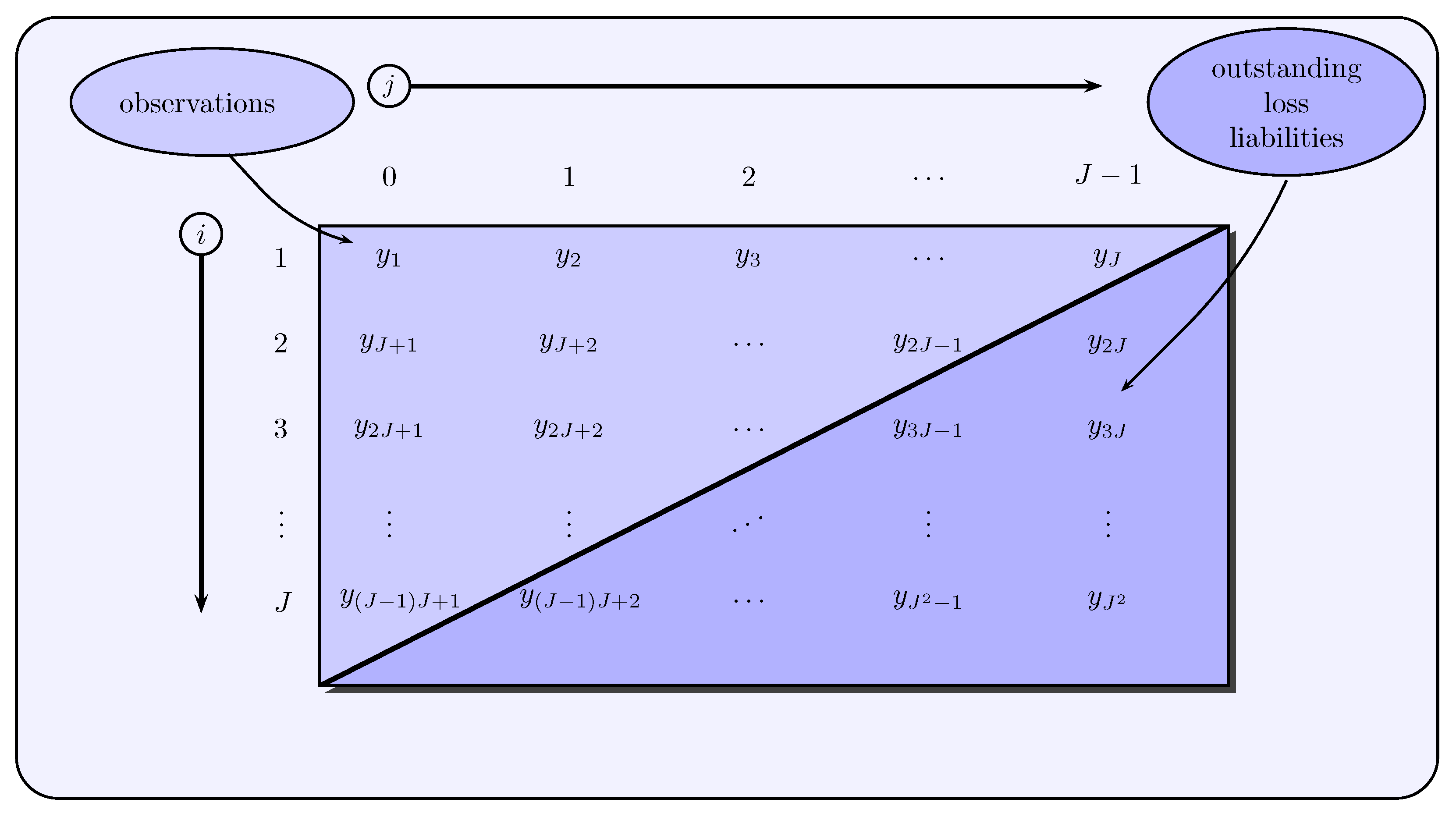
$⊳$ Forecasting the outstanding loss liabilities

As the system matrices ${\mathbf{G}}_t,{\mathbf{F}}_t,{\mathbf{B}}_t$ are assumed to be known for all $t=1,\dots ,I$, the outstanding loss liabilities for individual and aggregated accident years can be predicted by using ${\widehat{\mathbf{x}}}_{I|I}$ and ${\mathbf{P}}_{I|I}=\mathrm{Cov}\left({\mathbf{x}}_I-{\widehat{\mathbf{x}}}_{I|I}\right)$ in a straightforward way. To this end, all future incremental payments are collected in the vector

$$\begin{array}{c}\hfill {\mathbf{y}}_{I+1}={\left(\begin{array}{ccccccccc}{X}_{I,1}& X_{I-1,2}& \dots & X_{2,I-1}& X_{I,2}& \dots & X_{3,I-1}& \dots & X_{I,I-1}\end{array}\right)}^T.\end{array}$$

All these future observations belong to one of the accident years $i=2,\dots ,I$, and therefore, they are based on the corresponding state $\mathbf{b}\left(2\right),\dots ,\mathbf{b}\left(I\right)$. Accordingly, the state vector ${\mathbf{x}}_{I+1}$ corresponds to the vector ${\mathbf{x}}_I$ of the current calendar year I, which is why the state Equation (15) is given by ${\mathbf{x}}_{I+1}={\mathbf{x}}_I$ (i.e., ${\mathbf{F}}_{I+1}=\mathbf{I}$, ${\mathbf{Q}}_{I+1}=\mathbf{O}$). The system matrix ${\mathbf{G}}_{I+1}$ of the observation equation is obtained on the basis of (1) similar to that in (8), i.e., it consists mostly of zero vectors, and the entries ${\mathbf{\varphi }}^T\left(j\right)$ with $j=1,\dots ,I-1$ are ordered such that they are multiplied by the states $\mathbf{b}\left(i\right)$ from ${\mathbf{x}}_I$ of the corresponding accident year $i=1,\dots ,I$ of $X_{i,j}$ from ${\mathbf{y}}_{I+1}$. Thus, the future observations can be predicted via

$$\begin{array}{cc}\hfill {\widehat{\mathbf{y}}}_{I+1|I}& ={\mathbf{G}}_{I+1}{\widehat{\mathbf{x}}}_{I|I}\hfill \end{array}$$

(given by (9)) and

$$\begin{array}{c}\hfill \left(\begin{array}{c}{\widehat{X}}_{I,1}\\ {\widehat{X}}_{I-1,2}\\ ⋮\\ {\widehat{X}}_{2,I-1}\\ {\widehat{X}}_{I,2}\\ ⋮\\ {\widehat{X}}_{3,I-1}\\ ⋮\\ {\widehat{X}}_{I,I-1}\end{array}\right)=\left(\begin{array}{ccccc}{\mathbf{\varphi }}^T\left(1\right)& {\mathbf{0}}^T& \dots & \dots & {\mathbf{0}}^T\\ {\mathbf{0}}^T& {\mathbf{\varphi }}^T\left(2\right)& & & ⋮\\ ⋮& & \ddots & & ⋮\\ {\mathbf{0}}^T& \dots & {\mathbf{0}}^T& {\mathbf{\varphi }}^T(I-1)& ⋮\\ {\mathbf{\varphi }}^T\left(2\right)& {\mathbf{0}}^T& \dots & \dots & ⋮\\ ⋮& \ddots & & & ⋮\\ {\mathbf{0}}^T& \dots & {\mathbf{\varphi }}^T(I-1)& {\mathbf{0}}^T& ⋮\\ ⋮& & & & ⋮\\ {\mathbf{\varphi }}^T(I-1)& {\mathbf{0}}^T& \dots & \dots & {\mathbf{0}}^T\end{array}\right)\left(\begin{array}{c}\widehat{\mathbf{b}}\left(I\right)\\ \widehat{\mathbf{b}}(I-1)\\ ⋮\\ \widehat{\mathbf{b}}\left(1\right)\end{array}\right),\end{array}$$

respectively. The variance–covariance matrix of the prediction error $\left({\mathbf{y}}_{I+1}-{\widehat{\mathbf{y}}}_{I+1|I}\right)$ is given by:

$$\begin{array}{c}\hfill {\Delta }_{I+1}=\mathrm{Cov}\left({\mathbf{y}}_{I+1}-{\widehat{\mathbf{y}}}_{I+1|I}\right)={\mathbf{G}}_{I+1}{\mathbf{P}}_{I|I}{\mathbf{G}}_{I+1}^T\end{array}$$

Since ${\widehat{\mathbf{x}}}_{I|I}$, ${\mathbf{P}}_{I|I}$, ${\mathbf{G}}_{I+1}$ are known at time $t=I$, a prediction of the outstanding loss liabilities for individual and aggregated accident years is straightforward. With respect to the aggregated accident years, all components from ${\widehat{\mathbf{y}}}_{I+1|I}$ are to be added to the total loss reserve, while for individual accident years only those components from ${\widehat{\mathbf{y}}}_{I+1|I}$ related to the respective accident year $i=2,\dots ,I$ are to be added. An extraction of these components can be carried out via a diagonal matrix $\mathbf{A}$, which has a value of one at the respective positions and otherwise zeros. The variance–covariance matrix belonging to $\mathbf{A}{\widehat{\mathbf{y}}}_{I+1|I}$ is thus

$$\begin{array}{c}\hfill \mathrm{Cov}\left(\mathbf{A}{\mathbf{y}}_{I+1}-\mathbf{A}{\widehat{\mathbf{y}}}_{I+1|I}\right)=\mathbf{A}{\Delta }_{I+1}{\mathbf{A}}^T.\end{array}$$

However, if the modified payment stream according to (2) is used, additional uncertainty is induced via the inflation index $\lambda \left(t\right)$ of future calendar years $t>I$, which is unknown at time $t=I$. This is due to the unknown entries $n\left(i\right)\lambda (i+j){\mathbf{\varphi }}^T\left(j\right)$ for $i+j>I$ instead of the known entries ${\mathbf{\varphi }}^T\left(j\right)$ in the system matrix ${\mathbf{G}}_{I+1}$.

2.2. A Stochastic Method for Claims Reserving in General Insurance

Wright (1990) primarily establishes a model for incremental payments that includes a state space approach, where the variation of the parameters is modeled over different accident years. Thus, although the model of Wright (1990) is not mainly based on state space models and the Kalman filter theory, it embeds them in a model framework as one component. In the following, therefore, the model for incremental payments and the state space model are presented (for further details, see Wright 1990).

$⊳$ Construction of the model for claims payments

The modeling is built on development triangles that include incremental payments $X_{i,j}$ in accident years $i=1,\dots ,I$ and development years $j=0,\dots ,I-1$. The proposed model is based on the assumption that incremental payments $X_{i,j}$ are composed of the sum of $N_{i,j}$ independent and identically distributed (i.i.d.) payments $X_{i,j}^k$ (which are stochastically independent of $N_{i,j}$), that is, $X_{i,j}={\sum }_{k=1}^{N_{i,j}}{X}_{i,j}^k$. Thus, Wright (1990) uses the collective risk model and $X_{i,j}$ has a mixture distribution (see, e.g., Kaas et al. 2009). The lags j of individual incremental payments $X_{i,j}^k$ between the accident year of the claim and the actual payment are modeled as i.i.d. random variables, which is why $p_{i,j}$ with ${\sum }_{j=0}^{I-1}{p}_{i,j}=1$ is defined as the probability of payments regarding claims of accident year i in a given development year j. Let the number $N_{i,j}$ of payments for claims of accident year i in development year j be Poisson-distributed with parameter ${\epsilon }_i{p}_{i,j}$, i.e., $N_{i,j}\sim P\left({\epsilon }_i{p}_{i,j}\right)$; then, the incremental payments $X_{i,j}$ follow a mixture Poisson distribution. Following the convolution property of the Poisson distribution, the total number of claims payments $N_i={\sum }_{j=0}^{I-1}{N}_{i,j}$ of an accident year i also follows a Poisson distribution with parameter

$$\begin{array}{c}\hfill {\epsilon }_i=\sum _{j=0}^{I-1}{\epsilon }_i{p}_{i,j},\end{array}$$

where the $N_{i,j}$ for different j are assumed to be stochastically independent random variables and the parameter ${\epsilon }_i$ serves as a measure for the exposure of accident year i. As for modeling of the probability $p_{i,j}$, Wright (1990) gives two alternatives, the stochastic CL and the Hoerl curve model. While in the first alternative it is assumed that the probabilities $p_{i,j}$ are identical over all accident years i, the second alternative (preferred by Wright 1990) provides a modeling via a Hoerl curve of the form

$$\begin{array}{c}\hfill p_{i,j}={\alpha }_j{\kappa }_i{j}^{\prime A_i}{e}^{-B_i{j}^{\prime }}\end{array}$$

(17)

with constants ${\kappa }_i$, $A_i$ and $B_i$ to be estimated and ${\alpha }_j$ and $j^{\prime }$ as functions depending on j. Using (17), the expected value and variance of $N_{i,j}$ are as follows:

$$\begin{array}{c}\hfill \mathbb{E}\left[N_{i,j}\right]=\mathrm{Var}\left(N_{i,j}\right)={\epsilon }_i{p}_{i,j}={\epsilon }_i{\alpha }_j{\kappa }_i{j}^{\prime A_i}{e}^{-B_i{j}^{\prime }}\end{array}$$

(18)

In addition to the number $N_{i,j}$ of payments, Wright (1990) also models the amount of individual payments $X_{i,j}^k$ for claims of an accident year i in the j-th development year, which, like the $N_{i,j}$, are also assumed to be stochastically independent for various j. The first two moments of $X_{i,j}^k$ are modeled distribution-free with help of

$$\begin{array}{c}\hfill \mathbb{E}\left[X_{i,j}^k\right]=e^{{\delta }_t}K{j}^{\prime \lambda }\mathrm{and}\mathrm{Var}\left(X_{i,j}^k\right)={\rho }^2\mathbb{E}{\left[X_{i,j}^k\right]}^2\end{array}$$

(19)

with proper (unknown) constants $K>0$, $\lambda$, $\rho$ and inflation parameter ${\delta }_t$. While such a modeling of the expected value with different $\lambda$ and K provides a variety of possibilities, the modeling of the variance results from the assumption that the coefficient of variation

$$\begin{array}{c}\hfill \mathrm{CV}=\frac{\sqrt{\mathrm{Var}\left(X_{i,j}^k\right)}}{\mathbb{E}\left[X_{i,j}^k\right]}\end{array}$$

is time-invariant and corresponds to $\rho$. The optional term $e^{{\delta }_t}$ in (19) with

$$\begin{array}{c}\hfill {\delta }_t=\sum _{k=1}^t{\tau }_k\end{array}$$

and ${\tau }_k$ as the average annual inflation rate between calendar years $k-1$ and k, on the other hand, are used to account for inflation; i.e., $e^{{\delta }_t}$ reflects the inflation factor from the first calendar year to calendar year $t=i+j$. However, Wright (1990) proposes using

$$\begin{array}{c}\hfill {\delta }_t=\sum _{k=1}^t\tau =t\tau =(i+j)\tau \approx (i+j^{\prime })\tau ,\end{array}$$

(20)

and therefore assumes a constant inflation rate $\tau$.

Considering (18)–(20), and using the moments of the mixture Poisson distribution, the expected value and variance of the incremental payments $X_{i,j}$ in $(i,j)$ are obtained via

$$\begin{array}{c}\hfill \mathbb{E}\left[X_{i,j}\right]=\mathbb{E}\left[N_{i,j}\right]\mathbb{E}\left[X_{i,j}^k\right]={\epsilon }_i{p}_{i,j}{e}^{(i+j^{\prime })\tau }K{j}^{\prime \lambda }\end{array}$$

(21)

and

$$\begin{array}{cc}\hfill \mathrm{Var}\left(X_{i,j}\right)& =\mathbb{E}\left[N_{i,j}\right]\mathbb{E}\left[{\left(X_{i,j}^k\right)}^2\right]\hfill \\ \hfill & =\mathbb{E}\left[N_{i,j}\right]\left(\mathbb{E}{\left[X_{i,j}^k\right]}^2+\mathrm{Var}\left(X_{i,j}^k\right)\right)\hfill \\ \hfill & =\mathbb{E}\left[N_{i,j}\right]\left(1+{\rho }^2\right)\mathbb{E}{\left[X_{i,j}^k\right]}^2\hfill \\ \hfill & ={\epsilon }_i{p}_{i,j}\left(1+{\rho }^2\right)e^{2\tau (i+j^{\prime })}{K}^2{j}^{\prime 2\lambda },\hfill \end{array}$$

(22)

where $X_{i,j}$ are stochastically independent for different j due to the assumptions regarding $N_{i,j}$ and $X_{i,j}^k$. Moreover, Wright (1990) normalizes the incremental payments $X_{i,j}$ with the help of

$$\begin{array}{c}\hfill X_{i,j}^{\prime }=\frac{X_{i,j}}{{\tilde{\epsilon }}_i{\alpha }_j}\end{array}$$

(23)

with exposure defined by

$$\begin{array}{c}\hfill {\epsilon }_i={\tilde{\epsilon }}_i{\epsilon }_i^{\prime }.\end{array}$$

(24)

By using (17), (21), (23), (24), the expected value $\mathbb{E}\left[X_{i,j}^{\prime }\right]={\mu }_{i,j}^{\prime }$ of the normalized incremental payments $X_{i,j}^{\prime }$ can be stated as follows:

$$\begin{array}{cc}\hfill {\mu }_{i,j}^{\prime }& =\frac{1}{{\tilde{\epsilon }}_i{\alpha }_j}\mathbb{E}\left[X_{i,j}\right]\hfill \\ \hfill & =\frac{1}{{\tilde{\epsilon }}_i{\alpha }_j}{\epsilon }_i{p}_{i,j}{e}^{(i+j^{\prime })\tau }K{j}^{\prime \lambda }\hfill \\ \hfill & =\frac{1}{{\tilde{\epsilon }}_i{\alpha }_j}{\epsilon }_i{\alpha }_j{\kappa }_i{j}^{\prime A_i}{e}^{-B_i{j}^{\prime }}{e}^{(i+j^{\prime })\tau }K{j}^{\prime \lambda }\hfill \\ \hfill & =e^{i\tau }{\epsilon }_i^{\prime }{\kappa }_{i}K{j}^{\prime \left(A_i+\lambda \right)}{e}^{-(B_i-\tau )j^{\prime }}\hfill \\ \hfill & =e^{{\beta }_{i,1}}{j}^{\prime {\beta }_{i,2}}{e}^{-{\beta }_{i,3}{j}^{\prime }}\hfill \end{array}$$

(25)

with

$$\begin{array}{cc}\hfill {\beta }_{i,1}& =i\tau +ln\left({\epsilon }_i^{\prime }{\kappa }_{i}K\right)\hfill \\ \hfill {\beta }_{i,2}& =A_i+\lambda \hfill \\ \hfill {\beta }_{i,3}& =B_i-\tau \hfill \end{array}$$

Considering (22), (23), (25), the variance of $X_{i,j}^{\prime }$ is

$$\begin{array}{cc}\hfill \mathrm{Var}\left(X_{i,j}^{\prime }\right)& =\frac{1}{{\left({\tilde{\epsilon }}_i{\alpha }_j\right)}^2}\mathrm{Var}\left(X_{i,j}\right)\hfill \\ \hfill & =\frac{1}{{\left({\tilde{\epsilon }}_i{\alpha }_j\right)}^2}{\epsilon }_i{p}_{i,j}\left(1+{\rho }^2\right)e^{2\tau (i+j^{\prime })}{K}^2{j}^{\prime 2\lambda }\hfill \\ \hfill & ={\mu }_{i,j}^{\prime }\frac{1}{{\tilde{\epsilon }}_i{\alpha }_j}\left(1+{\rho }^2\right)e^{(i+j^{\prime })\tau }K{j}^{\prime \lambda }\hfill \\ \hfill & ={\mu }_{i,j}^{\prime }{\varphi }_i{\psi }_j\hfill \end{array}$$

with

$$\begin{array}{c}\hfill {\varphi }_i=\frac{K(1+{\rho }^2)e^{i\tau }}{{\tilde{\epsilon }}_i}\mathrm{and}{\psi }_j=\frac{j^{\prime \lambda }{e}^{j^{\prime }\tau }}{{\alpha }_j}.\end{array}$$

Assuming that ${\varphi }_i$ and ${\psi }_j$ are known, one obtains a generalized linear model of the form

$$\begin{array}{c}\hfill X_{i,j}^{\prime }={\mu }_{i,j}^{\prime }+e_{i,j}=exp\left({\mathbf{x}}_j^T{\mathbf{\beta }}_i\right)+e_{i,j}\end{array}$$

with the exponential response function $h^{-1}$, linear predictor ${\mathbf{x}}_j^T{\mathbf{\beta }}_i$ consisting of

$$\begin{array}{c}\hfill {\mathbf{x}}_j=\left(\begin{array}{c}1\\ ln\left(j^{\prime }\right)\\ -j^{\prime }\end{array}\right)\mathrm{and}{\mathbf{\beta }}_i=\left(\begin{array}{c}{\beta }_{i,1}\\ {\beta }_{i,2}\\ {\beta }_{i,3}\end{array}\right)\end{array}$$

and noise term $e_{i,j}$ with

$$\begin{array}{c}\hfill \mathbb{E}\left[e_{i,j}\right]=0\mathrm{and}\mathrm{Var}\left(e_{i,j}\right)={\mu }_{i,j}^{\prime }{\varphi }_i{\psi }_j,\end{array}$$

where the parameter estimators ${\widehat{\mathbf{\beta }}}_i$ and variance–covariance matrices ${\mathbf{R}}_i$ can be determined for all i using the Fisher scoring algorithm such that ${\mathbf{\beta }}_i\sim N\left({\widehat{\mathbf{\beta }}}_i;{\mathbf{R}}_i\right)$ is approximately satisfied. However, since ${\varphi }_i$ and ${\psi }_j$ are usually unknown, Wright (1990) proposes an iterative approach using parameter initializations to determine initial values for ${\varphi }_i$ and ${\psi }_j$. Considering this approach, all accident years are run sequentially and the results of all accident years are subsequently used to obtain new estimates of the parameters for the next run.

$⊳$ Modeling the parameter variation via a state space model

To increase the reliability of the estimators ${\widehat{\mathbf{\beta }}}_i$, Wright (1990) models the variation in the parameters ${\mathbf{\beta }}_i$ for different accident years i via

$$\begin{array}{c}\hfill {\mathbf{\beta }}_i={\mathbf{\beta }}_{i-1}+\left(\begin{array}{c}\tau \\ 0\\ 0\end{array}\right)+{\mathbf{\omega }}_i\end{array}$$

(26)

with

$$\begin{array}{c}\hfill {\mathbf{\omega }}_i=\left(\begin{array}{c}{\omega }_{i,1}\\ {\omega }_{i,2}\\ {\omega }_{i,3}\end{array}\right),\mathbb{E}\left[{\mathbf{\omega }}_i\right]=\mathbf{0}\mathrm{and}\mathrm{Cov}\left({\mathbf{\omega }}_i\right)=\left(\begin{array}{ccc}{u}_1^2& 0& 0\\ 0& u_2^2& 0\\ 0& 0& u_3^2\end{array}\right).\end{array}$$

By defining ${\mathbf{x}}_i$ with the help of

$$\begin{array}{c}\hfill {\mathbf{x}}_i={\left(\begin{array}{cccc}\tau & {\beta }_{i,1}& {\beta }_{i,2}& {\beta }_{i,3}\end{array}\right)}^T\end{array}$$

(27)

and by using (26), (27) can be written as

$$\begin{array}{c}\hfill {\mathbf{x}}_i={\mathbf{F}}_i{\mathbf{x}}_{i-1}+{\mathbf{v}}_i(\mathrm{state}\mathrm{equation})\end{array}$$

(28)

with

$$\begin{array}{c}\hfill {\mathbf{F}}_i=\left(\begin{array}{cccc}1& 0& 0& 0\\ 1& 1& 0& 0\\ 0& 0& 1& 0\\ 0& 0& 0& 1\end{array}\right),{\mathbf{x}}_{i-1}=\left(\begin{array}{c}\tau \\ {\beta }_{i-1,1}\\ {\beta }_{i-1,2}\\ {\beta }_{i-1,3}\end{array}\right)\mathrm{and}{\mathbf{v}}_i=\left(\begin{array}{c}0\\ {\omega }_{i,1}\\ {\omega }_{i,2}\\ {\omega }_{i,3}\end{array}\right),\end{array}$$

where $\mathbb{E}\left[{\mathbf{v}}_i\right]=\mathbf{0}$ and

$$\begin{array}{c}\hfill \mathbb{E}\left[{\mathbf{v}}_h{\mathbf{v}}_i^T\right]=\left\{\begin{array}{cc}{\mathbf{Q}}_i\hfill & \mathrm{i}\mathrm{f}h=i\hfill \\ \mathbf{O}\hfill & \mathrm{o}\mathrm{t}\mathrm{h}\mathrm{e}\mathrm{r}\mathrm{w}\mathrm{i}\mathrm{s}\mathrm{e}\hfill \end{array}\right.\end{array}$$

hold for all $h,i=1,\dots ,I$. Thus, Equation (28) forms the state equation of a state space model. Considering the estimators ${\widehat{\mathbf{\beta }}}_i$ as observations ${\mathbf{y}}_i$, the associated observation equation can be obtained via

$$\begin{array}{c}\hfill {\mathbf{y}}_i={\mathbf{G}}_i{\mathbf{x}}_i+{\mathbf{w}}_i(\mathrm{observation}\mathrm{equation})\end{array}$$

(29)

with

$$\begin{array}{c}\hfill {\mathbf{y}}_i=\left(\begin{array}{c}{\widehat{\beta }}_{i,1}\\ {\widehat{\beta }}_{i,2}\\ {\widehat{\beta }}_{i,3}\end{array}\right),{\mathbf{G}}_i=\left(\begin{array}{cccc}0& 1& 0& 0\\ 0& 0& 1& 0\\ 0& 0& 0& 1\end{array}\right),{\mathbf{w}}_i=\left(\begin{array}{c}{\epsilon }_{i,1}\\ {\epsilon }_{i,2}\\ {\epsilon }_{i,3}\end{array}\right)\end{array}$$

and $\mathbb{E}\left[{\mathbf{w}}_i\right]=\mathbf{0}$,

$$\begin{array}{c}\hfill \mathbb{E}\left[{\mathbf{w}}_h{\mathbf{w}}_i^T\right]=\left\{\begin{array}{cc}{\mathbf{R}}_i\hfill & \mathrm{i}\mathbf{f}h=i\hfill \\ \mathbf{O}\hfill & \mathrm{o}\mathrm{t}\mathrm{h}\mathrm{e}\mathrm{r}\mathrm{w}\mathrm{i}\mathrm{s}\mathrm{e}\hfill \end{array}\right.\end{array}$$

and $\mathbb{E}\left[{\mathbf{v}}_h{\mathbf{w}}_i^T\right]=\mathbf{O}$ for all $h,i=1,\dots ,I$. Accordingly, a complete state space model with $w=3$ and $v=4$ is specified via Equations (28) and (29).

2.3. Kalman Filters with Applications to Loss Reserving

Zehnwirth (1997) states that this article arose from various lecture notes on statistics and actuarial science and should be viewed primarily as an introduction to Kalman filter theory and ordinary least squares (OLS) estimation and their close relationship to Bayes estimation. Thus, Zehnwirth (1997) derives Kalman recursions for (multiple) linear regression models and the local level model, shows the connections of sample-based updates with Bayes updates in OLS estimators, and discusses state space models and the general Kalman filter algorithms.

The focus in the experimental and empirical applications is primarily not on an application of the Kalman filter, but on an investigation of the trend properties within claims development triangles. In the experimental application, a simulation of incremental payments $X_{i,j}$ in accident years $i=1,\dots ,I$ and development years $j=0,\dots ,I-1$ is performed via

$$\begin{array}{c}\hfill X_{i,j}=e^{\alpha -0.2j},\end{array}$$

(30)

i.e., a variation of the Hoerl curve. The factor $e^{\alpha }$ reflects the basic level of incremental payments, while the factor $e^{-0.2j}$ describes their decreasing behavior over the development years. Based on this, calendar year effects (in the form of inflation factors) are illustrated and the problem of overparameterization is addressed, which arises, e.g., when there are too many parameters for the individual accident years, but can be remedied by recursively evolving parameters. However, no specific state space representation is developed.

2.4. Loss Reserving: Past, Present and Future

Taylor et al. (2003) give a classification scheme for claims reserving methods whose higher-level criteria make a division between static and dynamic methods. In the framework of this taxonomic classification and especially with respect to the dynamic methods, they discuss a generalized Kalman filter, which allows for non-linearities in the observation equation and noise terms following a distribution of the Exponential Dispersion Family (EDF). They present two modeling approaches based on different types of claims data and state space representations constructed specifically for these data.

$⊳$ Accident year-based state space modeling

In the first modeling approach, an accident year-based state space representation is constructed, which is based on Payments Per Claim Incurred (PPCI) of a workers’ compensation insurance policy as claims data. The PPCI of an accident year $i=0,\dots ,I$ in the development year $j=0,\dots ,I$ are denoted by $Y_{i,j}$ and belong to the ($t=i+j$)-th calendar year with $t=0,\dots ,I$.

The state space model considered by Taylor et al. (2003) is based on a linear state equation of the form

$$\begin{array}{c}\hfill {\mathbf{x}}_{i+1}={\mathbf{F}}_i{\mathbf{x}}_i+{\mathbf{v}}_i(\mathrm{state}\mathrm{equation})\end{array}$$

(31)

with five-dimensional random vectors ${\mathbf{x}}_i,{\mathbf{v}}_i$, transition matrix ${\mathbf{F}}_i\in {\mathbb{R}}^{5\times 5}$, $\mathbb{E}\left[{\mathbf{v}}_i\right]=\mathbf{0}$ and

$$\begin{array}{c}\hfill \mathbb{E}\left[{\mathbf{v}}_i{\mathbf{v}}_k^T\right]=\left\{\begin{array}{cc}{\mathbf{Q}}_i\hfill & \mathrm{i}\mathrm{f}i=k\hfill \\ \mathbf{O}\hfill & \mathrm{o}\mathrm{t}\mathrm{h}\mathrm{e}\mathrm{r}\mathrm{w}\mathrm{i}\mathrm{s}\mathrm{e}\hfill \end{array}\right.\end{array}$$

for $i,k=0,\dots ,I-1$, while the observation equation

$$\begin{array}{c}\hfill {\mathbf{y}}_i=h^{-1}\left({\mathbf{G}}_i{\mathbf{x}}_i\right)+{\mathbf{w}}_i(\mathrm{observation}\mathrm{equation})\end{array}$$

(32)

with ($I-i+1$)-dimensional random vectors ${\mathbf{y}}_i,{\mathbf{w}}_i$, system matrix ${\mathbf{G}}_i\in {\mathbb{R}}^{(I-i+1)\times 5}$, $\mathbb{E}\left[{\mathbf{w}}_i\right]=\mathbf{0}$ and

$$\begin{array}{c}\hfill \mathbb{E}\left[{\mathbf{w}}_i{\mathbf{w}}_k^T\right]=\left\{\begin{array}{cc}{\mathbf{R}}_i\hfill & \mathrm{i}\mathrm{f}i=k\hfill \\ \mathbf{O}\hfill & \mathrm{o}\mathrm{t}\mathrm{h}\mathrm{e}\mathrm{r}\mathrm{w}\mathrm{i}\mathrm{s}\mathrm{e}\hfill \end{array}\right.\end{array}$$

is based on a generalized linear model with link function h (i.e., response function $h^{-1}$) and linear predictor ${\mathbf{G}}_i{\mathbf{x}}_i$ for all $i,k=0,\dots ,I$. Moreover, $\mathbb{E}\left[{\mathbf{v}}_i{\mathbf{w}}_k^T\right]=\mathbf{O}$ holds for all $i,k=0,\dots ,I$, the initial state ${\mathbf{x}}_0$ is uncorrelated with ${\mathbf{v}}_i$ and ${\mathbf{w}}_i$ for all $i=0,\dots ,I$ and ${\mathbf{w}}_i$ is assumed to be EDF-distributed for all $i=0,\dots ,I$. Thus, any strictly monotonic and differentiable link function h (such as a logarithm function) can be used to link the EDF-distributed observations ${\mathbf{y}}_i$ and the systematic component ${\mathbf{G}}_i{\mathbf{x}}_i$. The resulting recursive equations Taylor et al. (2003) refer to as the EDF filter, which include the Kalman filter as a special case, namely for the identity function as link function and normally distributed noise terms ${\mathbf{w}}_i$. The observation vector ${\mathbf{y}}_i$ in (32) includes all PPCIs of an accident year $i=0,\dots ,I$ of the upper claims development triangle (see Figure 4).

Figure 4. Accident year-based modeling of the observation vector.

Taylor et al. (2003) propose a logarithm function as a link function, the noise terms ${\mathbf{w}}_i$ are assumed to be gamma-distributed and the $(j+1)$-th row of the linear predictor ${\mathbf{G}}_i{\mathbf{x}}_i$ for an accident year $i=0,\dots ,I$ is given by

$$\begin{array}{c}\hfill {\beta }_{i,0}+{\beta }_{i,1}(j+1)+\frac{{\beta }_{i,2}}{j+1}+\frac{{\beta }_{i,3}}{{(j+1)}^2}+{\beta }_{i,4}{\delta }_{j,0}\end{array}$$

(33)

with respect to the development year $j=0,\dots ,I$. Here, ${\delta }_{j,0}$ denotes the Kronecker delta,

$$\begin{array}{c}\hfill {\delta }_{j,0}=\left\{\begin{array}{cc}1\hfill & \mathrm{if}j=0\hfill \\ 0\hfill & \mathrm{if}j>0\hfill \end{array}\right.,\end{array}$$

which can be used to model the peak in development year $j=0$. Thus, the observation Equation (32) of accident year $i=0,\dots ,I$ can be stated as follows:

$$\begin{array}{c}\hfill \left(\begin{array}{c}{Y}_{i,0}\\ Y_{i,1}\\ ⋮\\ Y_{i,j}\\ ⋮\\ Y_{i,I-i}\end{array}\right)=exp\left(\left(\begin{array}{ccccc}1& 1& 1& 1& 1\\ 1& 2& \frac{1}{2}& \frac{1}{4}& 0\\ ⋮& ⋮& ⋮& ⋮& ⋮\\ 1& j+1& \frac{1}{j+1}& \frac{1}{{(j+1)}^2}& 0\\ ⋮& ⋮& ⋮& ⋮& ⋮\\ 1& I-i+1& \frac{1}{I-i+1}& \frac{1}{{(I-i+1)}^2}& 0\end{array}\right)\left(\begin{array}{c}{\beta }_{i,0}\\ {\beta }_{i,1}\\ {\beta }_{i,2}\\ {\beta }_{i,3}\\ {\beta }_{i,4}\end{array}\right)\right)+\left(\begin{array}{c}{w}_{i,0}\\ w_{i,1}\\ ⋮\\ w_{i,j}\\ ⋮\\ w_{i,I-i}\end{array}\right)\end{array}$$

On the other hand, Taylor et al. (2003) do not provide any information on the concrete form of the state Equation (31). Taylor et al. (2003) model the evolution of the PPCI over the development years according to (33) in a similar way to De Jong and Zehnwirth (1983), Wright (1990) and Zehnwirth (1997), who specify the evolution of incremental payments over the development years with the help of a Hoerl curve. Taylor et al. (2003) apply this approach to the PPCI, as their evolution over the development years is similar to that of incremental payments: They reach their peak in development year $j=0$ and then drop relatively quickly to zero. This evolution of the PPCI is also the justification of Taylor et al. (2003) for the choice of the logarithm function as a link function and the assumption of a gamma distribution for the measurement noise.

$⊳$ Calendar year-based state space modeling

For the second modeling approach, Taylor et al. (2003) use a data set from Taylor (2000) that consists of motor vehicle bodily injury claim closure rates. Here, rather than collecting the observations from each accident year, they stack the observations from each calendar year into observation vectors. This is due to the fact that claim closure rates are relatively flat across development years, but are subject to calendar year effects.

The state space model proposed by Taylor et al. (2003) provides a linear state equation and an observation equation in the form of a generalized linear model, but differs from the first approach by the time index (calendar years t instead of accident years i) and by the matrix dimensions. They consider the following state space model consisting of the state equation

$$\begin{array}{c}\hfill {\mathbf{x}}_{t+1}={\mathbf{F}}_t{\mathbf{x}}_t+{\mathbf{v}}_t(\mathrm{state}\mathrm{equation})\end{array}$$

(34)

with ($3t+9$)-dimensional random vectors ${\mathbf{x}}_{t+1}$, ${\mathbf{v}}_t$, a ($3t+6$)-dimensional random vector ${\mathbf{x}}_t$ and transition matrix ${\mathbf{F}}_t\in {\mathbb{R}}^{(3t+9)\times (3t+6)}$ for $t=0,\dots ,I-1$, and the observation equation of the t-th calendar year

$$\begin{array}{c}\hfill {\mathbf{y}}_t=h^{-1}\left({\mathbf{G}}_t{\mathbf{x}}_t\right)+{\mathbf{w}}_t(\mathrm{observation}\mathrm{equation})\end{array}$$

(35)

with ($t+1$)-dimensional random vectors ${\mathbf{y}}_t$, ${\mathbf{w}}_t$, and $(t+1)\times (3t+6)$-dimensional system matrix ${\mathbf{G}}_t$ for $t=0,\dots ,I$, where the assumptions concerning the noise terms correspond to those of the first approach (transferred to calendar years).

Taylor et al. (2003) choose the identity function as a link function and the measurement noise is assumed to be normally distributed, which is why one obtains an ordinary linear observation equation and the usual linear Kalman filter can be used. This choice is motivated by the sufficiently high number of claims closures in the underlying claims data, and the assumption of an approximate normal distribution is justified by the central limit theorem, although the assumption of a discrete probability distribution such as the binomial distribution would be more appropriate. As for the development of the expected claim closure rate $\mathbb{E}\left[Z_{i,j}\right]$ with respect to the claims of an accident year $i=0,\dots ,I$ over the development years $j=0,\dots ,I$, Taylor et al. (2003) assume

$$\begin{array}{c}\hfill \mathbb{E}\left[Z_{i,j}\right]={\beta }_{i,0}+\frac{{\beta }_{i,1}}{j+1}+\frac{{\beta }_{i,2}}{{(j+1)}^2}+{\gamma }_t{\delta }_{i+j,t}\end{array}$$

(36)

with ${\gamma }_t$ as effect of the t-th calendar year and Kronecker Delta ${\delta }_{i+j,t}$. The observation vector

$$\begin{array}{c}\hfill {\mathbf{y}}_t={\left(\begin{array}{ccccc}{Z}_{0,t}& Z_{1,t-1}& Z_{2,t-2}& \dots & Z_{t,0}\end{array}\right)}^T\end{array}$$

of the t-th calendar year with $t=0,\dots ,I$ contains all $t+1$ claim closure rates $Z_{i,j}$ of the respective calendar year $t=i+j$ (see Figure 5), which is why the $(3t+6)$-dimensional state vector can be stated as

$$\begin{array}{c}\hfill {\mathbf{x}}_t={\left(\begin{array}{ccccc}{\mathbf{\beta }}_0^{*}& {\mathbf{\beta }}_1^{*}& \dots & {\mathbf{\beta }}_t^{*}& {\mathbf{\gamma }}_t\end{array}\right)}^T\end{array}$$

with

$$\begin{array}{cc}\hfill {\mathbf{\beta }}_i^{*}& ={\left(\begin{array}{ccc}{\beta }_{i,0}& {\beta }_{i,1}& {\beta }_{i,2}\end{array}\right)}^T\hfill \end{array}$$

(37)

$$\begin{array}{cc}\hfill {\mathbf{\gamma }}_t& ={\left(\begin{array}{ccc}{\gamma }_t& 0& 0\end{array}\right)}^T\hfill \end{array}$$

(38)

for $i=0,\dots ,t$.

Figure 5. Calendar year-based modeling of the observation vector.

While the state vector ${\mathbf{x}}_i$ in the first modeling approach only contains the parameters of the i-th accident year, the state vector ${\mathbf{x}}_t$ contains all parameters up to the t-th accident year plus the corresponding calendar year effect. This is due to the fact that the observations of the t-th calendar year pass through all accident years $i=0,\dots ,t$. The observation Equation (35) is thus given by

$$\begin{array}{c}\hfill \left(\begin{array}{c}{Z}_{0,t}\\ Z_{1,t-1}\\ Z_{2,t-2}\\ ⋮\\ Z_{t,0}\end{array}\right)=\left(\begin{array}{ccccc}{\mathbf{\alpha }}_t^T& {\mathbf{0}}^T& \dots & {\mathbf{0}}^T& {\mathbf{e}}^T\\ {\mathbf{0}}^T& {\mathbf{\alpha }}_{t-1}^T& & ⋮& ⋮\\ ⋮& & \ddots & {\mathbf{0}}^T& ⋮\\ {\mathbf{0}}^T& \dots & {\mathbf{0}}^T& {\mathbf{\alpha }}_0^T& {\mathbf{e}}^T\end{array}\right)\left(\begin{array}{c}{\mathbf{\beta }}_0^{*}\\ {\mathbf{\beta }}_1^{*}\\ ⋮\\ {\mathbf{\beta }}_t^{*}\\ {\mathbf{\gamma }}_t\end{array}\right)+\left(\begin{array}{c}{w}_{0,t}\\ w_{1,t-1}\\ w_{2,t-2}\\ ⋮\\ w_{t,0}\end{array}\right)\end{array}$$

with

$$\begin{array}{cc}\hfill {\mathbf{\alpha }}_j& ={\left(\begin{array}{ccc}1& \frac{1}{j+1}& \frac{1}{{(j+1)}^2}\end{array}\right)}^T,\hfill \\ \hfill \mathbf{e}& ={\left(\begin{array}{ccc}1& 0& 0\end{array}\right)}^T,\hfill \end{array}$$

${\mathbf{\beta }}_i^{*}$ according to (37) and ${\mathbf{\gamma }}_t$ according to (38) for all $i,j=0,\dots ,t$ as well as three-dimensional zero vectors $\mathbf{0}$. The state Equation (34) is then

$$\begin{array}{c}\hfill \left(\begin{array}{c}{\mathbf{\beta }}_0^{*}\\ ⋮\\ {\mathbf{\beta }}_t^{*}\\ {\mathbf{\beta }}_{t+1}^{*}\\ {\mathbf{\gamma }}_{t+1}\end{array}\right)=\left(\begin{array}{cccc}\mathbf{I}& \mathbf{O}& \dots & \mathbf{O}\\ \mathbf{O}& \ddots & & ⋮\\ ⋮& & \mathbf{I}& ⋮\\ ⋮& & \mathbf{I}& \mathbf{O}\\ \mathbf{O}& \dots & \mathbf{O}& \mathbf{I}\end{array}\right)\left(\begin{array}{c}{\mathbf{\beta }}_0^{*}\\ {\mathbf{\beta }}_1^{*}\\ ⋮\\ {\mathbf{\beta }}_t^{*}\\ {\mathbf{\gamma }}_t\end{array}\right)+\left(\begin{array}{c}\mathbf{0}\\ ⋮\\ \mathbf{0}\\ {\mathbf{v}}_t^{\left(\mathbf{\beta }\right)}\\ {\mathbf{v}}_t^{\left(\mathbf{\gamma }\right)}\end{array}\right)\end{array}$$

where $\mathbf{I}$ and $\mathbf{O}$ in ${\mathbf{F}}_t$ are identity and zero matrices of dimensions $3\times 3$, respectively, $\mathbf{0}$ in ${\mathbf{v}}_t$ are three-dimensional zero vectors and ${\mathbf{v}}_t^{\left(\mathbf{\beta }\right)}$, ${\mathbf{v}}_t^{\left(\mathbf{\gamma }\right)}$ are given as follows:

$$\begin{array}{cc}\hfill {\mathbf{v}}_t^{\left(\mathbf{\beta }\right)}& ={\left(\begin{array}{ccc}{v}_{t,0}& v_{t,1}& v_{t,2}\end{array}\right)}^T\hfill \\ \hfill {\mathbf{v}}_t^{\left(\mathbf{\gamma }\right)}& ={\left(\begin{array}{ccc}{v}_t^{\left(\gamma \right)}& 0& 0\end{array}\right)}^T\hfill \end{array}$$

Thus, the state equation involves a dynamic estimation of the parameters ${\mathbf{\beta }}_{t+1}^{*}$ and ${\gamma }_{t+1}$ via

$$\begin{array}{cc}\hfill {\mathbf{\beta }}_{t+1}^{*}& ={\mathbf{\beta }}_t^{*}+{\mathbf{v}}_t^{\left(\mathbf{\beta }\right)}\hfill \\ \hfill {\gamma }_{t+1}& ={\gamma }_t+v_t^{\left(\gamma \right)}\hfill \end{array}$$

for $t=0,\dots ,I-1$. Finally, Table 2 gives an overview of the dimensions of vectors and matrices in the state space models of Taylor et al. (2003).

Table 2. Dimensions in the state space models of Taylor et al. (2003).

Accident Year-Based Model		Calendar Year-Based Model
${\mathbf{y}}_i$	$(I-i+1)\times 1$	${\mathbf{y}}_t$	$(t+1)\times 1$
${\mathbf{x}}_{i+1}$	$5\times 1$	${\mathbf{x}}_{t+1}$	$(3t+9)\times 1$
${\mathbf{x}}_i$	$5\times 1$	${\mathbf{x}}_t$	$(3t+6)\times 1$
${\mathbf{w}}_i$	$(I-i+1)\times 1$	${\mathbf{w}}_t$	$(t+1)\times 1$
${\mathbf{v}}_i$	$5\times 1$	${\mathbf{v}}_t$	$(3t+9)\times 1$
${\mathbf{G}}_i$	$(I-i+1)\times 5$	${\mathbf{G}}_t$	$(t+1)\times (3t+6)$
${\mathbf{F}}_i$	$5\times 5$	${\mathbf{F}}_t$	$(3t+9)\times (3t+6)$
${\mathbf{R}}_i$	$(I-i+1)\times (I-i+1)$	${\mathbf{R}}_t$	$(t+1)\times (t+1)$
${\mathbf{Q}}_i$	$5\times 5$	${\mathbf{Q}}_t$	$(3t+9)\times (3t+9)$

2.5. The Application of State Space Model in Outstanding Claims Reserve

Pang and He (2012) largely adopt the second modeling approach from Taylor et al. (2003), but without integrating calendar year effects. They extend the state equation by including a further lag of the state vector. Accordingly, the state space model they consider is given by

$$\begin{array}{cccc}{\mathbf{y}}_t\hfill & ={\mathbf{G}}_t{\mathbf{x}}_t+{\mathbf{w}}_t\hfill & & (\mathrm{observation}\mathrm{equation})\hfill \end{array}$$

(39)

$$\begin{array}{cccc}\hfill {\mathbf{x}}_{t+1}& ={\mathbf{F}}_t{\mathbf{x}}_t+{\mathbf{H}}_t{\mathbf{x}}_{t-1}+{\mathbf{v}}_t\hfill & & (\mathrm{state}\mathrm{equation})\hfill \end{array}$$

(40)

with $\mathbb{E}\left[{\mathbf{w}}_t\right]=\mathbf{0}$, $\mathbb{E}\left[{\mathbf{v}}_t\right]=\mathbf{0}$,

$$\begin{array}{c}\hfill \mathbb{E}\left[{\mathbf{w}}_s{\mathbf{w}}_t^T\right]=\left\{\begin{array}{cc}{\mathbf{R}}_t\hfill & \mathrm{i}\mathrm{f}s=t\hfill \\ \mathbf{O}\hfill & \mathrm{o}\mathrm{t}\mathrm{h}\mathrm{e}\mathrm{r}\mathrm{w}\mathrm{i}\mathrm{s}\mathrm{e}\hfill \end{array}\right.\mathrm{and}\mathbb{E}\left[{\mathbf{v}}_s{\mathbf{v}}_t^T\right]=\left\{\begin{array}{cc}{\mathbf{Q}}_t\hfill & \mathrm{i}\mathrm{f}s=t\hfill \\ \mathbf{O}\hfill & \mathrm{o}\mathrm{t}\mathrm{h}\mathrm{e}\mathrm{r}\mathrm{w}\mathrm{i}\mathrm{s}\mathrm{e}\hfill \end{array}\right.\end{array}$$

for all $s,t=1,\dots ,I$. Table 3 gives an overview of the dimensions of vectors and matrices in the state space model of Pang and He (2012).

Table 3. Dimensions in the state space model of Pang and He (2012).

Vectors		Matrices
${\mathbf{y}}_t$	$t\times 1$	${\mathbf{G}}_t$	$t\times 4t$
${\mathbf{x}}_t$	$4t\times 1$	${\mathbf{F}}_t$	$(4t+4)\times 4t$
${\mathbf{w}}_t$	$t\times 1$	${\mathbf{H}}_t$	$(4t+4)\times (4t-4)$
${\mathbf{v}}_t$	$(4t+4)\times 1$	${\mathbf{R}}_t$	$t\times t$
		${\mathbf{Q}}_t$	$(4t+4)\times (4t+4)$

The observation vector ${\mathbf{y}}_t$ contains all observations $X_{i,j}$ of the t-th calendar year, i.e., all $X_{i,j}$ with $i+j-1=t$. However, the nature of the claims data is not obvious and the authors refer to it only as “times of compensation”. Therefore, in view of the magnitude of the observations and their modeling, claims data are assumed to be incremental payments. The expected incremental payments of an accident year $i=1,\dots ,I$ are assumed to have a parametric evolution over the development years $j=1,\dots ,I$ similar to (33) via

$$\begin{array}{c}\hfill \mathbb{E}\left[X_{i,j}\right]={\theta }_{i,1}(j+1)+\frac{{\theta }_{i,2}}{j+1}+\frac{{\theta }_{i,3}}{{(j+1)}^2}+{\theta }_{i,4}{\delta }_{j,1}\end{array}$$

(41)

with Kronecker Delta ${\delta }_{j,1}$. Thus, the observation Equation (39) of the t-th calendar year ($t=1,\dots ,I$) results in a similar form as achieved within the second modeling approach of Taylor et al. (2003),

$$\begin{array}{c}\hfill \left(\begin{array}{c}{X}_{1,t}\\ X_{2,t-1}\\ ⋮\\ X_{t,1}\end{array}\right)=\left(\begin{array}{cccc}{\mathbf{\alpha }}_t^T& {\mathbf{0}}^T& \dots & {\mathbf{0}}^T\\ {\mathbf{0}}^T& {\mathbf{\alpha }}_{t-1}^T& & ⋮\\ ⋮& & \ddots & {\mathbf{0}}^T\\ {\mathbf{0}}^T& \dots & {\mathbf{0}}^T& {\mathbf{\alpha }}_1^T\end{array}\right)\left(\begin{array}{c}{\mathbf{\theta }}_1^{*}\\ {\mathbf{\theta }}_2^{*}\\ ⋮\\ {\mathbf{\theta }}_t^{*}\end{array}\right)+\left(\begin{array}{c}{w}_{1,t}\\ w_{2,t-1}\\ ⋮\\ w_{t,1}\end{array}\right)\end{array}$$

with

$$\begin{array}{cc}\hfill {\mathbf{\alpha }}_j& ={\left(\begin{array}{cccc}j+1& \frac{1}{j+1}& \frac{1}{{(j+1)}^2}& {\delta }_{j,1}\end{array}\right)}^T\hfill \\ \hfill \mathbf{0}& ={\left(\begin{array}{cccc}0& 0& 0& 0\end{array}\right)}^T\hfill \\ \hfill {\mathbf{\theta }}_i^{*}& ={\left(\begin{array}{cccc}{\theta }_{i,1}& {\theta }_{i,2}& {\theta }_{i,3}& {\theta }_{i,4}\end{array}\right)}^T\hfill \end{array}$$

for all $i,j=1,\dots ,I$. Pang and He (2012) do not give the general representation of the state equation according to (40), but the reduced form

$$\begin{array}{cc}\hfill {\mathbf{\theta }}_{t+1}^{*}& ={\mathbf{F}}_t^{*}{\mathbf{\theta }}_t^{*}+{\mathbf{H}}_t^{*}{\mathbf{\theta }}_{t-1}^{*}+{\mathbf{v}}_t^{*}\hfill \end{array}$$

(42)

which solely contains the last four rows of (40) that are of interest. For the remaining $(4\times 4)$-dimensional parameter matrices, they assume scalar matrices ${\mathbf{F}}_t^{*}={\mu }_t\mathbf{I}$ and ${\mathbf{H}}_t^{*}={\eta }_t\mathbf{I}$ for all $t=1,\dots ,I$, which is why the state Equation (42) is given by:

$$\begin{array}{c}\hfill \left(\begin{array}{c}{\theta }_{t+1,1}\\ {\theta }_{t+1,2}\\ {\theta }_{t+1,3}\\ {\theta }_{t+1,4}\end{array}\right)=\left(\begin{array}{cccc}{\mu }_t& 0& 0& 0\\ 0& {\mu }_t& 0& 0\\ 0& 0& {\mu }_t& 0\\ 0& 0& 0& {\mu }_t\end{array}\right)\left(\begin{array}{c}{\theta }_{t,1}\\ {\theta }_{t,2}\\ {\theta }_{t,3}\\ {\theta }_{t,4}\end{array}\right)+\left(\begin{array}{cccc}{\eta }_t& 0& 0& 0\\ 0& {\eta }_t& 0& 0\\ 0& 0& {\eta }_t& 0\\ 0& 0& 0& {\eta }_t\end{array}\right)\left(\begin{array}{c}{\theta }_{t-1,1}\\ {\theta }_{t-1,2}\\ {\theta }_{t-1,3}\\ {\theta }_{t-1,4}\end{array}\right)+\left(\begin{array}{c}{v}_{t,1}\\ v_{t,2}\\ v_{t,3}\\ v_{t,4}\end{array}\right)\end{array}$$

If, on the other hand, one intends to express the state equation in the form (40), the upper $(4t\times 4t)$-dimensional part of ${\mathbf{F}}_t$ corresponds to an identity matrix, while the last four rows in the last four columns of ${\mathbf{F}}_t$ form the scalar matrix ${\mathbf{F}}_t^{*}={\mu }_t\mathbf{I}$ and otherwise contain zeros. The parameter matrix ${\mathbf{H}}_t$ has only zeros in the $(4t\times (4t-4\left)\right)$-dimensional upper part and also in the last four rows except for the last four columns, which correspond to the $(4\times 4)$-dimensional scalar matrix ${\mathbf{H}}_t^{*}={\eta }_t\mathbf{I}$. The noise vector ${\mathbf{v}}_t$ is equal to a zero vector in the first $4t$ rows and to the vector ${\mathbf{v}}_t^{*}$ in the remaining rows.

3. Log-Normal Models for Incremental Payments (Category 2)

This section presents articles in which incremental payments are assumed to be log-normally distributed and are modeled using a log-normal model:

▸

Verrall (1989): A State Space Representation of the Chain Ladder Linear Model;

▸

Verrall (1994): A Method for Modelling varying Run-Off Evolutions in Claims Reserving;

⊳

Ntzoufras and Dellaportas (2002): Bayesian Modelling of Outstanding Liabilities incorporating Claim Count Uncertainty;

⊳

Li (2006): Comparison of Stochastic Reserving Methods.

The articles of Verrall (1989, 1994) are presented in detail due to the fact that they are mainly based on the use of state space models and the Kalman filter learning theory (marked in the above listing with ▸), while the models in the papers of Ntzoufras and Dellaportas (2002) and Li (2006) are treated in a more concise form (marked in the above listing with ⊳).

3.1. A State Space Representation of the Chain Ladder Linear Model

Verrall (1989) discusses various state space representations based on the model of a two-way ANOVA, and thus follows Kremer (1982), who shows a close connection between the CL method and the two-way ANOVA. In addition to a dynamic estimation of the parameters by means of the Kalman filter algorithms, Verrall (1989) also considers static models without and with prior information.

$⊳$ The linear Chain Ladder model

The modeling is based on increments $X_{i,j}>0$ with $i,j=1,\dots ,I$. The restriction to positive values is necessary against the backdrop of a logarithmic transformation of $X_{i,j}$. In practice, the model of Verrall (1989) can be applied to paid data, but not to incurred data. For the increments $X_{i,j}$, a multiplicative model

$$\begin{array}{c}\hfill X_{i,j}=u_i{s}_j{r}_{i,j}\end{array}$$

(43)

with $u_i$ as a parameter of the accident year i, $s_j$ as a parameter of the development year j and $r_{i,j}$ as noise term with $\mathbb{E}\left[r_{i,j}\right]=1$ for all $i,j=1,\dots ,I$ is assumed. Further, the increments are presumed to follow a log-normal distribution, so a logarithmic transformation of the increments is performed, i.e., $Y_{i,j}=log\left(X_{i,j}\right)$. Thus, the variables $Y_{i,j}$ are normally distributed. If both sides of (43) of the multiplicative model are logarithmized, this leads to the (additive) model of the two-way ANOVA with normally distributed residuals

$$\begin{array}{c}\hfill Y_{i,j}=\mu +{\alpha }_i+{\beta }_j+w_{i,j}\end{array}$$

(44)

with population mean $\mu$, row parameter ${\alpha }_i$, column parameter ${\beta }_j$ and $w_{i,j}\sim WN\left(0;{\sigma }^2\right)$ for all $i,j=1,\dots ,I$. As for the model parameters, Verrall (1989) assumes ${\alpha }_1={\beta }_1=0$ and

$$\begin{array}{cc}\hfill {\alpha }_i& =log\left(u_i\right)-log\left(u_1\right)\hfill \\ \hfill {\beta }_j& =log\left(s_j\right)-log\left(s_1\right)\hfill \\ \hfill \mu & =log\left(u_1\right)+log\left(s_1\right)\hfill \end{array}$$

with $i,j=2,\dots ,I$, and it holds $w_{i,j}=log\left(r_{i,j}\right)$ for all $i,j=1,\dots ,I$. Due to the fact that (44) is a model for logarithmized increments, it is referred to in the actuarial literature as log-normal model. Verrall (1989), on the other hand, chooses to refer to it as linear CL model because it is very similar to the CL method (in an additive representation). Kremer (1982) shows this similarity of the classical CL method to the two-way ANOVA by estimating the parameters of the model (44) via OLS estimation for the two-way ANOVA and then reversing the logarithmic transformations. The predictor for the ultimate claim of an accident year $i=1,\dots ,I$,

$$\begin{array}{c}\hfill \widehat{C_{i,I}}=e^{\widehat{\mu }}{e}^{{\widehat{\alpha }}_i}\prod _{j=1}^I{e}^{{\widehat{\beta }}_j},\end{array}$$

(45)

is similar to the CL predictor except for a different parameterization. However, Verrall (1989) argues that (45) is neither an MLE nor an unbiased estimator of the expected ultimate claim, so he proposes using Bayes estimators instead. In addition, Verrall (1989) develops several state space representations of the linear CL model (44), which are in the focus in the following.

$⊳$ Development of an appropriate state space representation

In order to specify a state space representation and to be able to use dynamic estimation methods, the linear CL model has to be specified in a recursive form. For this purpose, Verrall (1989) collected the incremental payments of a calendar year $t=1,\dots ,I$ in the t-dimensional vector ${\mathbf{y}}_t$. However, different from De Jong and Zehnwirth (1983), he did not use the available observations $X_{i,j}$, but the logarithmized observations $Y_{i,j}=log\left(X_{i,j}\right)$:

$$\begin{array}{c}\hfill {\mathbf{y}}_t={\left(\begin{array}{cccccc}{Y}_{1,t}& Y_{2,t-1}& Y_{3,t-2}& \dots & Y_{t-1,2}& Y_{t,1}\end{array}\right)}^T\end{array}$$

Hence, the entries $Y_{i,j}$, $i+j-1=t$, of the t-th diagonal are arranged in the observation vector of the t-th calendar year from top right to bottom left (i.e., opposite to De Jong and Zehnwirth 1983); see Figure 6.

Figure 6. Modeling the observation vector in Verrall (1989).

Using a state vector containing the model parameters $\mu ,{\alpha }_2,\dots ,{\alpha }_t,{\beta }_2,\dots ,{\beta }_t$ up to the t-th accident and development year, an appropriate observation equation for the t-th calendar year based on (44) can be stated as

$$\begin{array}{c}\hfill \left(\begin{array}{c}{Y}_{1,t}\\ Y_{2,t-1}\\ Y_{3,t-2}\\ ⋮\\ Y_{t-1,2}\\ Y_{t,1}\end{array}\right)=\left(\begin{array}{cccccccccccc}1& 0& \dots & & & & & & & \dots & 0& 1\\ 1& 1& 0& \dots & & & & \dots & 0& 1& 0& 0\\ 1& 0& 0& 1& 0& \dots & 0& 1& 0& 0& 0& 0\\ ⋮& & & & & \ddots & & & & & & ⋮\\ ⋮& & & & & & \ddots & & & & & ⋮\\ 1& 0& 1& 0& \dots & & \dots & 0& 1& 0& 0& 0\\ 1& 0& \dots & & & & & & \dots & 0& 1& 0\end{array}\right)\left(\begin{array}{c}\mu \\ {\alpha }_2\\ {\beta }_2\\ ⋮\\ {\alpha }_t\\ {\beta }_t\end{array}\right)+\left(\begin{array}{c}{w}_{1,t}\\ w_{2,t-1}\\ w_{3,t-2}\\ ⋮\\ w_{t-1,2}\\ w_{t,1}\end{array}\right)\end{array}$$

or in a more compact form as

$$\begin{array}{c}\hfill {\mathbf{y}}_t={\mathbf{G}}_t{\mathbf{x}}_t+{\mathbf{w}}_t(\mathrm{observation}\mathrm{equation})\end{array}$$

(46)

with t-dimensional observation vector ${\mathbf{y}}_t$, system matrix ${\mathbf{G}}_t\in {\mathbb{R}}^{t\times (2t-1)}$, $(2t-1)$-dimensional state vector ${\mathbf{x}}_t$, and t-dimensional Gaussian white noise process ${\left({\mathbf{w}}_t\right)}_{t=1,\dots ,I}$ with $\mathbb{E}\left[{\mathbf{w}}_t\right]=\mathbf{0}$ and

$$\begin{array}{c}\hfill \mathbb{E}\left[{\mathbf{w}}_s{\mathbf{w}}_t^T\right]=\left\{\begin{array}{cc}{\mathbf{R}}_t\hfill & \mathrm{i}\mathrm{f}s=t\hfill \\ \mathbf{O}\hfill & \mathrm{o}\mathrm{t}\mathrm{h}\mathrm{e}\mathrm{r}\mathrm{w}\mathrm{i}\mathrm{s}\mathrm{e}\hfill \end{array}\right.\end{array}$$

for all $s,t=1,\dots ,I$. For the third calendar year, for instance, (46) results in:

$$\begin{array}{cc}\hfill \left(\begin{array}{c}{Y}_{1,3}\\ Y_{2,2}\\ Y_{3,1}\end{array}\right)& =\left(\begin{array}{ccccc}1& 0& 0& 0& 1\\ 1& 1& 1& 0& 0\\ 1& 0& 0& 1& 0\end{array}\right)\left(\begin{array}{c}\mu \\ {\alpha }_2\\ {\beta }_2\\ {\alpha }_3\\ {\beta }_3\end{array}\right)+\left(\begin{array}{c}{w}_{1,3}\\ w_{2,2}\\ w_{3,1}\end{array}\right)\hfill \end{array}$$

(47)

For the state equation, Verrall (1989) gives several alternatives, where the most general variant is

$$\begin{array}{c}\hfill {\mathbf{x}}_{t+1}={\mathbf{F}}_t{\mathbf{x}}_t+{\mathbf{B}}_t{\mathbf{u}}_t+{\mathbf{v}}_t(\mathrm{state}\mathrm{equation})\end{array}$$

(48)

with system matrices ${\mathbf{F}}_t\in {\mathbb{R}}^{(2t+1)\times (2t-1)}$, ${\mathbf{B}}_t\in {\mathbb{R}}^{(2t+1)\times u}$, the u-dimensional stochastic input vector ${\mathbf{u}}_t\sim N\left({\widehat{\mathbf{u}}}_t;{\mathbf{U}}_t\right)$ as well as the $(2t+1)$-dimensional Gaussian white noise process ${\left({\mathbf{v}}_t\right)}_{t=1,\dots ,I}$ with $\mathbb{E}\left[{\mathbf{v}}_t\right]=\mathbf{0}$ and

$$\begin{array}{c}\hfill \mathbb{E}\left[{\mathbf{v}}_s{\mathbf{v}}_t^T\right]=\left\{\begin{array}{cc}{\mathbf{Q}}_t\hfill & \mathrm{i}\mathrm{f}s=t\hfill \\ \mathbf{O}\hfill & \mathrm{o}\mathrm{t}\mathrm{h}\mathrm{e}\mathrm{r}\mathrm{w}\mathrm{i}\mathrm{s}\mathrm{e}\hfill \end{array}\right.\end{array}$$

for $s,t=1,\dots ,I-1$. Here, ${\mathbf{w}}_t$, ${\mathbf{v}}_t$, ${\mathbf{u}}_t$ are pairwise stochastically independent for all $t=1,\dots ,I$ and the input vector ${\mathbf{u}}_t$ is independent of the state vector ${\mathbf{x}}_t$. Table 4 gives an overview of the dimensions of the vectors and matrices in the state space model of Verrall (1989).

Table 4. Dimensions in the state space model of Verrall (1989).

Vectors		Matrices
${\mathbf{y}}_t$	$t\times 1$	${\mathbf{G}}_t$	$t\times (2t-1)$
${\mathbf{x}}_t$	$(2t-1)\times 1$	${\mathbf{F}}_t$	$(2t+1)\times (2t-1)$
${\mathbf{u}}_t$	$u\times 1$	${\mathbf{B}}_t$	$(2t+1)\times u$
${\mathbf{w}}_t$	$t\times 1$	${\mathbf{R}}_t$	$t\times t$
${\mathbf{v}}_t$	$(2t+1)\times 1$	${\mathbf{Q}}_t$	$(2t+1)\times (2t+1)$

The dynamics of the system depend on the matrices ${\mathbf{F}}_t$, ${\mathbf{Q}}_t$ and the distribution of the input vector ${\mathbf{u}}_t$ in the state Equation (48). The simplest case is when ${\mathbf{u}}_t$ and ${\mathbf{v}}_t$ are zero vectors for all $t=1,\dots ,I$ and the parameters at time $t+1$ are the same as those at time t. Then, (48) is given by:

$$\begin{array}{cc}\hfill {\mathbf{x}}_{t+1}& =\left(\begin{array}{cccc}1& 0& \dots & 0\\ 0& \ddots & & ⋮\\ ⋮& & \ddots & 0\\ 0& \dots & 0& 1\\ 0& \dots & 1& 0\\ 0& \dots & 0& 1\end{array}\right){\mathbf{x}}_t\hfill \end{array}$$

(49)

If, on the other hand, one wants to realize different parameters at time $t+1$ and t, the following variant of the state Equation (48) can be used:

$$\begin{array}{cc}\hfill {\mathbf{x}}_{t+1}& =\left(\begin{array}{cccc}1& 0& \dots & 0\\ 0& \ddots & & ⋮\\ ⋮& & \ddots & 0\\ 0& \dots & 0& 1\\ 0& \dots & \dots & 0\\ 0& \dots & \dots & 0\end{array}\right){\mathbf{x}}_t+\left(\begin{array}{cc}0& 0\\ ⋮& ⋮\\ 0& 0\\ 1& 0\\ 0& 1\end{array}\right)\left(\begin{array}{c}{\alpha }_{t+1}\\ {\beta }_{t+1}\end{array}\right)\hfill \end{array}$$

(50)

The variation of the state Equation (50) means that already determined parameters remain unchanged and the new parameters are considered as stochastic inputs. While static parameter estimation is performed in the cases (49) and (50), dynamic parameter estimation can be achieved using the Kalman filter when a stochastic noise term ${\mathbf{v}}_t$ is added. For dynamic modeling, Verrall (1989) proposes state equations for two cases, for a dynamic estimation of the row parameters and for a dynamic estimation of both row and column parameters simultaneously. A dynamic estimation of the row parameters with help of the random walk ${\alpha }_{t+1}={\alpha }_t+v_t$ can be achieved via the following state equation:

$$\begin{array}{cc}\hfill {\mathbf{x}}_{t+1}& =\left(\begin{array}{cccc}1& 0& \dots & 0\\ 0& \ddots & & ⋮\\ ⋮& & \ddots & 0\\ 0& \dots & 0& 1\\ 0& \dots & 1& 0\\ 0& \dots & \dots & 0\end{array}\right){\mathbf{x}}_t+\left(\begin{array}{c}0\\ ⋮\\ 0\\ 0\\ 0\\ 1\end{array}\right){\beta }_{t+1}+\left(\begin{array}{c}0\\ ⋮\\ 0\\ 0\\ v_t\\ 0\end{array}\right)\hfill \end{array}$$

(51)

If, on the other hand, a dynamic estimation of both the row and column parameters according to the random walks

$$\begin{array}{c}\hfill \begin{array}{c}\hfill {\alpha }_{t+1}={\alpha }_t+v_t\\ \hfill {\beta }_{t+1}={\beta }_t+w_t\end{array}\end{array}$$

(52)

is intended, an input vector is obsolete and a reasonable state equation can be stated as follows:

$$\begin{array}{cc}\hfill {\mathbf{x}}_{t+1}& =\left(\begin{array}{cccc}1& 0& \dots & 0\\ 0& \ddots & & ⋮\\ ⋮& & \ddots & 0\\ 0& \dots & 0& 1\\ 0& \dots & 1& 0\\ 0& \dots & 0& 1\end{array}\right){\mathbf{x}}_t+\left(\begin{array}{c}0\\ ⋮\\ 0\\ 0\\ v_t\\ w_t\end{array}\right)\hfill \end{array}$$

(53)

Thus, dynamic parameter estimation is just between the identical and the different parameter cases, where the parameters in $t+1$ are related to the parameters in t, but do not necessarily have to match. The state Equation (53), which allows for a dynamic estimation of both row and column parameters, is also exemplarily given for $t=3$:

$$\begin{array}{c}\hfill {\mathbf{x}}_4=\left(\begin{array}{c}\mu \\ {\alpha }_2\\ {\beta }_2\\ {\alpha }_3\\ {\beta }_3\\ {\alpha }_4\\ {\beta }_4\end{array}\right)=\left(\begin{array}{ccccc}1& 0& 0& 0& 0\\ 0& 1& 0& 0& 0\\ 0& 0& 1& 0& 0\\ 0& 0& 0& 1& 0\\ 0& 0& 0& 0& 1\\ 0& 0& 0& 1& 0\\ 0& 0& 0& 0& 1\end{array}\right)\left(\begin{array}{c}\mu \\ {\alpha }_2\\ {\beta }_2\\ {\alpha }_3\\ {\beta }_3\end{array}\right)+\left(\begin{array}{c}0\\ 0\\ 0\\ 0\\ 0\\ v_3\\ w_3\end{array}\right)\end{array}$$

3.2. A Method for Modelling Varying Run-Off Evolutions in Claims Reserving

Verrall (1994) adopts the state space model presented in the work of Verrall (1989) with the aim to model a not necessarily homogeneous run-off evolution across the accident years within the CL method. With this approach, he addresses one of the main criticisms of the CL method, the homogeneity property. Since the state space model from Verrall (1989) is a linear CL model according to (44), Verrall (1994) shows how this model can be adjusted when there is a varying development pattern across accident years.

$⊳$ Connection between CL factors and column parameters

A possible method to model a not necessarily homogeneous run-off evolution across the accident years is, for example, to use the individual CL factors $F_{i,j}$ for all $i,j$ instead of the CL development factors $f_j$. Such modeling would allow for deviating development factors in different accident years, but comes with the disadvantage of overparameterization. It is therefore reasonable to strike a balance between both these extremes, i.e., between the CL development factors that are identical across the accident years and individual CL factors. For this purpose, Verrall (1994) uses the connection

$$\begin{array}{c}\hfill f_{j-1}=1+\frac{e^{{\beta }_j}}{{\sum }_{k=1}^{j-1}{e}^{{\beta }_k}}\end{array}$$

(54)

between the CL factors and the column parameters ${\beta }_j$ in the linear CL model (44) (see Verrall 1991) to be able to indirectly relax the homogeneity property of the CL method via modifications to the linear CL model.

$⊳$ Development of an appropriate state space representation

Verrall (1994) modifies the linear CL model of Verrall (1989) such that the column parameters ${\beta }_j$ with $j=2,\dots ,I$ need not to be identical across all accident years. He differentiates the parameters ${\beta }_j$ by accident years $i=1,\dots ,I$ via an extension of the notation to ${\beta }_{i,j}$, where ${\beta }_{i,j}$ corresponds to the column parameter ${\beta }_j$ in the i-th accident year. Verrall (1994) does not give general definitions of the observation and state equations, but in the following we provide such representations. As for the observation equation in the t-th calendar year, it can be given in general form as follows:

$$\begin{array}{c}\hfill \left(\begin{array}{c}{Y}_{1,t}\\ Y_{2,t-1}\\ Y_{3,t-2}\\ ⋮\\ Y_{t-1,2}\\ Y_{t,1}\end{array}\right)=\left(\begin{array}{cccccccccccc}1& 0& \dots & & & & & & & \dots & 0& 1\\ 1& 1& 0& \dots & & & & \dots & 0& 1& 0& 0\\ 1& 0& 0& 1& 0& \dots & 0& 1& 0& 0& 0& 0\\ ⋮& & & & & \ddots & & & & & & ⋮\\ ⋮& & & & & & \ddots & & & & & ⋮\\ 1& 0& 1& 0& \dots & & \dots & 0& 1& 0& 0& 0\\ 1& 0& \dots & & & & & & \dots & 0& 1& 0\end{array}\right)\left(\begin{array}{c}\mu \\ {\alpha }_2\\ {\beta }_{t-1,2}\\ ⋮\\ {\alpha }_t\\ {\beta }_{1,t}\end{array}\right)+\left(\begin{array}{c}{w}_{1,t}\\ w_{2,t-1}\\ w_{3,t-2}\\ ⋮\\ w_{t-1,2}\\ w_{t,1}\end{array}\right)\end{array}$$

As an example, the observation equation in $t=3$ results in:

$$\begin{array}{cc}\hfill \left(\begin{array}{c}{Y}_{1,3}\\ Y_{2,2}\\ Y_{3,1}\end{array}\right)& =\left(\begin{array}{ccccc}1& 0& 0& 0& 1\\ 1& 1& 1& 0& 0\\ 1& 0& 0& 1& 0\end{array}\right)\left(\begin{array}{c}\mu \\ {\alpha }_2\\ {\beta }_{2,2}\\ {\alpha }_3\\ {\beta }_{1,3}\end{array}\right)+\left(\begin{array}{c}{w}_{1,3}\\ w_{2,2}\\ w_{3,1}\end{array}\right)\hfill \end{array}$$

A connection between the parameters of successive accident years can be established by the state Equation (48). In this regard, a dynamic estimation of the row parameters can be achieved via

$$\begin{array}{c}\hfill {\alpha }_{i+1}={\alpha }_i+v_i\end{array}$$

(55)

with ${\alpha }_1=0$ and $\mathbb{E}\left[v_i\right]=0$ for all $i=1,\dots ,I-1$ to avoid overparameterization of the model. The column parameters ${\beta }_{i,j}$ of a development year j are supposed to be connected across accident years i in such a way that they follow a random walk

$$\begin{array}{c}\hfill {\beta }_{i,j}={\beta }_{i-1,j}+v_{i,j}\end{array}$$

(56)

with ${\beta }_{i,1}=0$, ${\beta }_{0,j}=0$ and $\mathbb{E}\left[v_{i,j}\right]=0$ for all $i=1,\dots ,I$ and $j=2,\dots ,I$. In this manner, it is found that the parameters related to a specific development year are similar for different accident years or can be identical, but do not necessarily have to be identical. If one assumes a variance of zero for the noise terms $v_{i,j}$ for all $i,j$, one obtains the state Equation (51) from Verrall (1989), i.e., the column parameters ${\beta }_{i,j}$ of development year j are identical across all considered accident years i and correspond to the column parameter ${\beta }_j$ of the linear CL model (44). The larger the variance of the noise terms $v_{i,j}$ chosen, the larger the variation in the parameters ${\beta }_{i,j}$ can be across different accident years. Accordingly, the variances of the individual noise terms can be used to account for the indicators of changes in the development pattern.

Thus, the state equation is obtained using (55) and (56):

$$\begin{array}{c}\hfill \left(\begin{array}{c}\mu \\ {\alpha }_2\\ {\beta }_{t,2}\\ {\alpha }_3\\ {\beta }_{t-1,3}\\ ⋮\\ {\alpha }_t\\ {\beta }_{2,t}\\ {\alpha }_{t+1}\\ {\beta }_{1,t+1}\end{array}\right)=\left(\begin{array}{cccccccc}1& 0& \dots & & & & \dots & 0\\ 0& 1& 0& \dots & & & \dots & 0\\ 0& 0& 1& 0& \dots & & \dots & 0\\ 0& 0& 0& 1& 0& \dots & \dots & 0\\ 0& 0& 0& 0& 1& 0& \dots & 0\\ ⋮& & & & & \ddots & & ⋮\\ 0& \dots & & & \dots & 0& 1& 0\\ 0& \dots & & & \dots & 0& 0& 1\\ 0& \dots & & & \dots & 0& 1& 0\\ 0& \dots & & & \dots & 0& 0& 0\end{array}\right)\left(\begin{array}{c}\mu \\ {\alpha }_2\\ {\beta }_{t-1,2}\\ {\alpha }_3\\ {\beta }_{t-2,3}\\ ⋮\\ {\alpha }_{t-1}\\ {\beta }_{2,t-1}\\ {\alpha }_t\\ {\beta }_{1,t}\end{array}\right)+\left(\begin{array}{c}0\\ 0\\ 0\\ 0\\ 0\\ ⋮\\ 0\\ 0\\ 0\\ 1\end{array}\right){\beta }_{1,t+1}+\left(\begin{array}{c}0\\ 0\\ v_{t,2}\\ 0\\ v_{t-1,3}\\ ⋮\\ 0\\ v_{2,t}\\ v_t\\ 0\end{array}\right)\end{array}$$

Considering $t=3$, the state equation is exemplarily given by:

$$\begin{array}{c}\hfill \left(\begin{array}{c}\mu \\ {\alpha }_2\\ {\beta }_{3,2}\\ {\alpha }_3\\ {\beta }_{2,3}\\ {\alpha }_4\\ {\beta }_{1,4}\end{array}\right)=\left(\begin{array}{ccccc}1& 0& 0& 0& 0\\ 0& 1& 0& 0& 0\\ 0& 0& 1& 0& 0\\ 0& 0& 0& 1& 0\\ 0& 0& 0& 0& 1\\ 0& 0& 0& 1& 0\\ 0& 0& 0& 0& 0\end{array}\right)\left(\begin{array}{c}\mu \\ {\alpha }_2\\ {\beta }_{2,2}\\ {\alpha }_3\\ {\beta }_{1,3}\end{array}\right)+\left(\begin{array}{c}0\\ 0\\ 0\\ 0\\ 0\\ 0\\ 1\end{array}\right){\beta }_{1,4}+\left(\begin{array}{c}0\\ 0\\ v_{3,2}\\ 0\\ v_{2,3}\\ v_3\\ 0\end{array}\right)\end{array}$$

Finally, when estimates of the column parameters ${\beta }_{i,j}$ for all $i,j$ are obtained (determined by means of the Kalman filter), the individual CL factors $F_{i,j}$ can be determined separately for individual accident years via

$$\begin{array}{c}\hfill F_{i,j-1}=1+\frac{e^{{\beta }_{i,j}}}{{\sum }_{k=1}^{j-1}{e}^{{\beta }_{i,k}}}\end{array}$$

according to (54) for $j=2,\dots ,I$. In this manner, a not necessarily homogeneous run-off evolution across all accident years can be modeled within the CL method and the problem of overparameterization is avoided due to the recursive development of the column parameters. Furthermore, it should be emphasized that a dynamic estimation of the parameters has a considerable advantage over the static CL estimation: the observations of more recent accident years have a higher weight with respect to the prediction of the outstanding loss liabilities, whereas CL assigns the same weight to all the observations.

3.3. Bayesian Modelling of Outstanding Liabilities Incorporating Claim Count Uncertainty

Ntzoufras and Dellaportas (2002) consider four models based on claims development triangles that include incremental payments and claim counts for RBNS claims. They assume that claims are settled via one-off payments. They justify this assumption by means of their empirical application example, in which they use run-off data from a large Greek motor insurance company, where claims must be reported within three working days according to Greek legislation and are usually settled in the form of a one-off payment. The proportion of claims that are paid in more than one installment of claims payments is minimal, and therefore is neglected by Ntzoufras and Dellaportas (2002).

Two models are based solely on incremental payments, while the other two models incorporate incremental payments and claim counts, thus using Payments Per Claim Finalized (PPCF). Ntzoufras and Dellaportas (2002) adjust the incremental payments $X_{i,j}$ by the inflation index ${\nu }_{i,j}\ge 1$ of the corresponding calendar year $t=i+j-1$ and log-transform the inflation-adjusted incremental payments that are assumed to be log-normally distributed via

$$\begin{array}{c}\hfill Y_{i,j}=log\left(\frac{X_{i,j}}{{\nu }_{i,j}}\right),\end{array}$$

such that $Y_{i,j}\sim N\left({\mu }_{i,j};{\sigma }^2\right)$ for all $i,j=1,\dots ,I$. The definition of $\mathbb{E}\left[Y_{i,j}\right]={\mu }_{i,j}$ is different for the four models under consideration:

⊳

Log-normal model for incremental payments (Model 1);

⊳

Log-normal model for PPCF (Model 2);

⊳

State space model for incremental payments (Model 3);

⊳

State space model for PPCF (Model 4).

but it is generally based on the two-way ANOVA model and thus also on the linear CL model from Verrall (1989, 1994) according to (44). In the framework of models 3 and 4, Ntzoufras and Dellaportas (2002) consider state space models; however, they only specify the ANOVA model, recursive relationships of the parameters and model extensions without developing a specific state space representation. The reason for this is that they do not employ the Kalman filter to fit the model and to predict the outstanding loss liabilities, but instead they use a Bayesian approach in combination with Markov Chain Monte Carlo (MCMC). As the article by Ntzoufras and Dellaportas (2002) does not mainly rely on state space models and the Kalman filter theory, the models are presented briefly, and, in particular, details on the Bayesian approach are omitted.

$⊳$ Log-normal model for incremental payments (Model 1)

The log-normal model for incremental payments, where the expected value ${\mu }_{i,j}$ is given by

$$\begin{array}{c}\hfill {\mu }_{i,j}=\mu +{\alpha }_i+{\beta }_j\end{array}$$

(57)

for all $i,j=1,\dots ,I$ with ${\alpha }_1={\beta }_1=0$, is already considered by various authors. That is, the expected incremental payments ${\mu }_{i,j}$ for claims of the i-th accident year that are paid with a lag of $j-1$ years are modeled via a linear predictor. This predictor consists of the sum of $\mu$ (expected inflation- and log-adjusted claims payments of the first accident year that are settled in the same development year), ${\alpha }_i$ (row parameter reflecting expected changes in the ith accident year), and ${\beta }_j$ (column parameter reflecting expected changes in the jth development year). According to Ntzoufras and Dellaportas (2002), the ANOVA model has the disadvantage that it includes only one source of information (i.e., incremental payments) and omits claims counts. For example, this model would not be able to take into account a strong increase in incremental payments due to a surprising increase in the claim counts.

$⊳$ Log-normal model for PPCF (Model 2)

The log-normal model for PPCF extends the first model by additionally considering claim counts in the modeling. For this purpose, Ntzoufras and Dellaportas (2002) give a two-stage model, where the first stage is related to incremental payments,

$$\begin{array}{c}\hfill {\mu }_{i,j}=\mu +{\alpha }_i+{\beta }_j+log\left(N_{i,j}\right)\end{array}$$

(58)

with ${\alpha }_1={\beta }_1=0$ and claim counts $N_{i,j}>0$ for all $i,j=1,\dots ,I$. Compared with model 1, the ANOVA model (57) was additively extended by the term $log\left(N_{i,j}\right)$, which is why $\mu$ in (58) can be interpreted as the logarithmized expected PPCF of the first accident year in the first development year, and the parameters ${\alpha }_i$ and ${\beta }_j$ can be considered as expected deviations from $\mu$ in the later accident and development years, respectively. The second stage of the model is related to the claim counts $N_{i,j}\sim P\left({\lambda }_{i,j}\right)$ with ${\lambda }_{i,j}>0$. It is given by the log-linear model

$$\begin{array}{c}\hfill log\left({\lambda }_{i,j}\right)={\mu }^{*}+{\alpha }_i^{*}+{\beta }_j^{*}\end{array}$$

with constraints ${\sum }_{j=1}^I{N}_{i,j}=T_i$, ${\sum }_{j=1}^I{\lambda }_{i,j}=T_i$ for all $i,j=1,\dots ,I$, hyper-parameters ${\mu }^{*}$ and ${\alpha }_i^{*}$, and ${\beta }_j^{*}=log\left(\frac{{\pi }_j}{{\pi }_1}\right)$, where ${\alpha }_1^{*}={\beta }_1^{*}=0$ holds, $0<{\pi }_j<1$ is the probability that a claim will be settled with a lag of $j-1$ years, and $T_i$ denotes the total number of claims for a given accident year i. In this model, an increase in incremental payments induced by higher claim counts is accounted for.

$⊳$ State space model for incremental payments (Model 3)

The state space model for incremental payments is based on the discussion of Verrall (1989) and the extension of the column parameters ${\beta }_j$ to ${\beta }_{i,j}$ as proposed by Verrall (1994):

$$\begin{array}{c}\hfill {\mu }_{i,j}=\mu +{\alpha }_i+{\beta }_{i,j}\end{array}$$

Here, the row and column parameters ${\alpha }_i$ and ${\beta }_{i,j}$ follow the recursions

$$\begin{array}{cc}\hfill {\alpha }_i& ={\alpha }_{i-1}+h_i\hfill \end{array}$$

(59)

$$\begin{array}{cc}\hfill {\beta }_{i,j}& ={\beta }_{i-1,j}+v_i\hfill \end{array}$$

(60)

with $h_i\sim N\left(0;{\sigma }_h^2\right)$ and $v_i\sim N\left(0;{\sigma }_v^2\right)$ as well as ${\alpha }_1={\beta }_{i,1}=0$ for all $i,j=2,\dots ,I$. Thus, for the variance of the individual log-transformed and inflation-adjusted incremental payments $Y_{i,j}$, $\mathrm{Var}\left(Y_{i,j}\right)={\sigma }^2$ holds for $i=1$ or $j=1$ and $\mathrm{Var}\left(Y_{i,j}\right)={\sigma }^2+(i-1)\left({\sigma }_v^2+{\sigma }_h^2\right)$ holds for $i,j=2,\dots ,I$, as in each subsequent accident year after accident year $i=1$, the weighted sum of the variance terms ${\sigma }_v^2$, ${\sigma }_h^2$ (see recursions (59) and (60)) is added to the variance term ${\sigma }^2$. That is, this model differs from model 1 in two ways: the column parameters ${\beta }_j$ are extended to ${\beta }_{i,j}$, and both row and column parameters evolve recursively. The recursions (59) and (60) are thereby decisively affected by the variances ${\sigma }_h^2$ and ${\sigma }_v^2$ of their noise terms: If ${\sigma }_h^2$ is assumed to be close to zero, all row parameters tend to zero due to ${\alpha }_1=0$. If, on the other hand, ${\sigma }_v^2=0$ is assumed, models 1 and 3 are identical (except for the $\alpha$-recursion) because the column parameters are the same across all accident years, i.e., ${\beta }_{i,j}={\beta }_j$ holds for all i.

$⊳$ State space model for PPCF (Model 4)

The state space model for PPCF extends model 3 by incorporating claim counts. Like the second model, it is designed as a two-stage model, with stage 1 related to incremental payments and stage 2 related to claim counts. Thus, the first stage of model 4 is described via

$$\begin{array}{c}\hfill {\mu }_{i,j}=\mu +{\alpha }_i+{\beta }_{i,j}+log\left(N_{i,j}\right)\end{array}$$

for all $i,j=1,\dots ,I$ with recursions (59) and (60), and the second stage is identical to the second stage of model 2. Hence, like models 1 and 3, models 2 and 4 differ in other column parameters and in the recursive relationships of row and column parameters.

3.4. Comparison of Stochastic Reserving Methods

Li (2006) compares some methods in stochastic claims reserving, including a state space model, in terms of forecasting the outstanding loss liabilities. The considered state space model

$$\begin{array}{cccc}\hfill {\mathbf{y}}_t& ={\mathbf{G}}_t{\mathbf{x}}_t+{\mathbf{w}}_t\hfill & & (\mathrm{observation}\mathrm{equation})\hfill \end{array}$$

(61)

$$\begin{array}{cccc}\hfill {\mathbf{x}}_t& ={\mathbf{F}}_t{\mathbf{x}}_{t-1}+{\mathbf{v}}_t\hfill & & (\mathrm{state}\mathrm{equation})\hfill \end{array}$$

(62)

is based on the common assumptions regarding the noise terms (as, for example, in De Jong and Zehnwirth 1983), and it is constructed in analogy to Verrall (1989) via the log-normal model for incremental payments and the linear CL model (44), respectively: the observation vector ${\mathbf{y}}_t$ includes all logarithmized incremental payments $Y_{i,j}=log\left(X_{i,j}\right)$ with $X_{i,j}>0$ of the t-th calendar year ($t=i+j-1$ with $i,j=1,\dots ,I$), where the $Y_{i,j}$ have an expected value of $\mathbb{E}\left[Y_{i,j}\right]=\mu +{\alpha }_i+{\beta }_j$ with ${\alpha }_1={\beta }_1=0$. The measurement noise $w_{i,j}$ that overlays the expected logarithmized incremental payments follows a Gaussian white noise process ($w_{i,j}\sim WN\left(0;{\sigma }_w^2\right)$). The state vector ${\mathbf{x}}_t$ includes $\mu$, row parameters ${\alpha }_2,\dots ,{\alpha }_t$, and column parameters ${\beta }_2,\dots ,{\beta }_I$; thus, unlike Verrall (1989), column parameters beyond $j=t$ for $t<I$ are also included. Table 5 gives an overview of the dimensions of the vectors and matrices in the state space model of Li (2006).

Table 5. Dimensions in the state space model of Li (2006).

Vectors		Matrices
${\mathbf{y}}_t$	$t\times 1$	${\mathbf{G}}_t$	$t\times (t+I-1)$
${\mathbf{x}}_t$	$(t+I-1)\times 1$	${\mathbf{F}}_t$	$(t+I-1)\times (t+I-2)$
${\mathbf{w}}_t$	$t\times 1$	${\mathbf{R}}_t$	$t\times t$
${\mathbf{v}}_t$	$(t+I-1)\times 1$	${\mathbf{Q}}_t$	$(t+I-1)\times (t+I-1)$

The observation Equation (61) of the t-th calendar year can be stated as:

$$\begin{array}{c}\hfill \left(\begin{array}{c}{Y}_{1,t}\\ Y_{2,t-1}\\ ⋮\\ Y_{t,1}\end{array}\right)=\left(\begin{array}{ccccccccccc}1& 0& \dots & \dots & \dots & \dots & \dots & 0& 1& 0& \dots \\ 1& \ddots & & & & & & ⋰& 0& 0& \dots \\ ⋮& & \ddots & & & & ⋰& & ⋮& 0& \dots \\ 1& & & \ddots & & ⋰& & & 0& 0& \dots \\ 1& 0& \dots & 0& 1& 0& \dots & 0& 0& 0& \dots \end{array}\right)\left(\begin{array}{c}\mu \\ {\alpha }_2\\ ⋮\\ {\alpha }_t\\ {\beta }_2\\ ⋮\\ {\beta }_I\end{array}\right)+\left(\begin{array}{c}{w}_{1,t}\\ w_{2,t-1}\\ ⋮\\ w_{t,1}\end{array}\right)\end{array}$$

The part on the left-hand side of the vertical line in the system matrix ${\mathbf{G}}_t$ is generally of dimensions $t\times (2t-1)$, and the part on the right-hand side consists of $(I-t)$ zero columns for all $t=1,\dots ,I$. Thus, if $t=I$, ${\mathbf{G}}_t$ only includes the $(I\times (2I-1\left)\right)$-dimensional part on the left-hand side of the vertical line and no zero columns. As for the state Equation (62), Li (2006) proposes a dynamic estimation of the row parameters according to ${\alpha }_t={\alpha }_{t-1}+v_t$ with $v_t\sim WN\left(0;{\sigma }_v^2\right)$ for $t\ge 2$:

$$\begin{array}{c}\hfill \left(\begin{array}{c}\mu \\ {\alpha }_2\\ ⋮\\ {\alpha }_t\\ {\beta }_2\\ ⋮\\ {\beta }_I\end{array}\right)=\left(\begin{array}{cccccc}1& 0& \dots & & \dots & 0\\ 0& \ddots & & & & ⋮\\ ⋮& & 1& & & \\ & & 1& & & \\ & & & 1& & ⋮\\ ⋮& & & & \ddots & 0\\ 0& \dots & & \dots & 0& 1\end{array}\right)\left(\begin{array}{c}\mu \\ {\alpha }_2\\ ⋮\\ {\alpha }_{t-1}\\ {\beta }_2\\ ⋮\\ {\beta }_I\end{array}\right)+\left(\begin{array}{c}0\\ ⋮\\ 0\\ v_t\\ 0\\ ⋮\\ 0\end{array}\right)\end{array}$$

(63)

For $t\ge 3$, the $(t-1)$-th column of ${\mathbf{F}}_t$ thus contains in the rows $t-1$ and t the value one and otherwise only zeros. In the case $t=2$, however, ${\mathbf{F}}_t$ deviates from (63) by having only zeros in the second row because of ${\alpha }_2=v_2$. The noise term $v_t$ corresponds in each case to the t-th component of the vector ${\mathbf{v}}_t$.

4. Correlation Models (Category 3)

This section presents two articles:

⊳

De Jong (2005): State Space Models in Actuarial Science;

▸

De Jong (2006): Forecasting Runoff Triangles.

Here, correlations regarding the different dimensions of claims development triangles are considered. As the conference paper by De Jong (2005) can be seen as a preprint of De Jong (2006) (with respect to the remarks on claims reserving), it is briefly presented, while De Jong (2006) is highlighted in the listing (as in the previous sections) with ▸ since it is significantly based on state space models and Kalman filter learning theory.

4.1. State Space Models in Actuarial Science

De Jong (2005) discusses two applications of state space models in actuarial sciences, in relation to mortality and in relation to cumulative payments in run-off triangles. As for the latter one, he extends the model of Hertig (1985) and proposes the so-called development correlation model. This model is already presented in a prior working paper by De Jong (2004), where two additional models, the accident correlation model and the calendar correlation model, are proposed, but without discussing their state space representations. This extension, i.e., an embedding of the three models into state space representations and model fitting via Kalman filter, is carried out in the work of De Jong (2006). Thus, with respect to applications of state space models in claims reserving, De Jong (2005) is a variant of De Jong (2006), which only deals with one of the correlation models. For this reason, we refer to the following subsection, in which the article of De Jong (2006) is presented.

4.2. Forecasting Runoff Triangles

De Jong (2006) aims to predict the outstanding loss liabilities using three different models that can account for correlations within the claims data. In each case, De Jong (2006) gives state space representations for these models in order to be able to apply the Kalman filter to predict the claims reserves and to quantify their precision. Based on these results, he simulates the complete shape of the liability distribution. In the following, the focus is mainly on the state space representations of the considered models.

The proposed correlation models in the work of De Jong (2006) are generally based on a model of Hertig (1985), which is extended in such a way that correlations between the individual accident, development or calendar years can be incorporated into the modeling. The models consider the logarithmized individual development factors

$$\begin{array}{c}\hfill {\delta }_{i,j}=ln\left(\frac{C_{i,j}}{C_{i,j-1}}\right)\end{array}$$

(64)

with $i=1,\dots ,I$, $j=1,\dots ,I-1$ and ${\delta }_{i,0}=ln\left(C_{i,0}\right)$. Using the individual development factors (64), the future growth rate $g_i$ of cumulative payments in each accident year $i=2,\dots ,I$ can be decomposed as follows:

$$\begin{array}{cc}{g}_i\hfill & =ln\left({\displaystyle \frac{C_{i,I-1}}{C_{i,I-i}}}\right)\hfill \\ \hfill & =ln\left({\displaystyle \frac{C_{i,I-i+1}}{C_{i,I-i}}}·{\displaystyle \frac{C_{i,I-i+2}}{C_{i,I-i+1}}}\cdots {\displaystyle \frac{C_{i,I-1}}{C_{i,I-2}}}\right)\hfill \\ \hfill & =ln\left({\displaystyle \frac{C_{i,I-i+1}}{C_{i,I-i}}}\right)+ln\left({\displaystyle \frac{C_{i,I-i+2}}{C_{i,I-i+1}}}\right)+\dots +ln\left({\displaystyle \frac{C_{i,I-1}}{C_{i,I-2}}}\right)\hfill \\ \hfill & ={\delta }_{i,I-i+1}+\dots +{\delta }_{i,I-1}\hfill \end{array}$$

(65)

Considering (65), the outstanding loss liabilities $R_i=C_{i,I-1}-C_{i,I-i}$ of an accident year $i=2,\dots ,I$ are given by:

$$\begin{array}{c}\hfill R_i=C_{i,I-i}\left(e^{g_i}-1\right)\end{array}$$

(66)

An aggregation of (66) across all accident years yields the total outstanding loss liabilities:

$$\begin{array}{c}\hfill R=\sum _{i=2}^I{R}_i=\sum _{i=2}^I{C}_{i,I-i}\left(e^{g_i}-1\right)\end{array}$$

(67)

Thus, in order to predict the outstanding loss liabilities, it is necessary to estimate the growth rates $g_2,\dots ,g_I$ according to (65) and the future logarithmized individual development factors ${\delta }_{i,j}$ for $i+j>I$, respectively. For this purpose, De Jong (2006) considers three extended variants of the model proposed by Hertig (1985). The model of Hertig (1985),

$$\begin{array}{c}\hfill {\delta }_{i,j}={\mu }_j+h_j{\epsilon }_{i,j}\end{array}$$

(68)

with $h_0=1$, $\mathbb{E}\left[{\epsilon }_{i,j}\right]=0$ and $\mathrm{Var}\left({\epsilon }_{i,j}\right)={\sigma }^2$, is a simple model for logarithmized individual development factors in which the ${\delta }_{i,j}$ are assumed to be uncorrelated for all $i=1,\dots ,I$, $j=0,\dots ,I-1$. Here, $\mathbb{E}\left[{\delta }_{i,j}\right]={\mu }_j$ and $\mathrm{Var}\left({\delta }_{i,j}\right)=h_j^2{\sigma }^2$, i.e., expected value and variance of the logarithmized individual development factors ${\delta }_{i,j}$ only depend on the development year j.

With the goal to incorporate correlations of the logarithmized individual development factors into the model of Hertig (1985), De Jong (2006) presents the development, accident, and calendar correlation models, each considering correlations between development years j, accident years i, and calendar years $t=i+j$, respectively. In order to achieve appropriate state space representations of these models, De Jong (2006) generally suggests the state space model

$$\begin{array}{cccc}\hfill {\mathbf{y}}_t& ={\mathbf{G}}_t{\mathbf{x}}_t+{\mathbf{H}}_t\mathbf{u}+{\mathbf{M}}_t{\mathbf{w}}_t\hfill & & (\mathrm{observation}\mathrm{equation})\hfill \end{array}$$

(69)

$$\begin{array}{cccc}\hfill {\mathbf{x}}_{t+1}& ={\mathbf{F}}_t{\mathbf{x}}_t+{\mathbf{B}}_t\mathbf{u}+{\mathbf{N}}_t{\mathbf{w}}_t\hfill & & (\mathrm{state}\mathrm{equation})\hfill \end{array}$$

(70)

with $t=1,\dots ,I$, where the t-dimensional observation vector ${\mathbf{y}}_t={\left({\delta }_{1,t-1},\dots ,{\delta }_{t,0}\right)}^T$ contains the logarithmized individual development factors ${\delta }_{i,j}$ of the t-th calendar year (see Figure 7).

Figure 7. Modeling of the observation vector in De Jong (2006).

Due to the fact that De Jong (2006) aims to embed all three models into the same general state space model, the state space representations obtained in this way are excessive in their complexity. This is in contrast to the underlying compact models, in particular the development correlation model with only one model equation.

$⊳$ Development correlation model

The development correlation model allows to model correlations of ${\delta }_{i,j}$ across development years $j=0,\dots ,I-1$ for a given accident year $i=1,\dots ,I$ and is defined by

$$\begin{array}{c}\hfill {\delta }_{i,j}={\mu }_j+h_j\left({\epsilon }_{i,j}+{\theta }_j{\epsilon }_{i,j-1}\right)\end{array}$$

(71)

with $\mathbb{E}\left[{\epsilon }_{i,j}{\epsilon }_{i,j-1}\right]=0$ for $i=1,\dots ,I$ and $j=1,\dots ,I-1$. Here, the correlation between development years j and $j-1$ (i.e., between ${\delta }_{i,j}$ and ${\delta }_{i,j-1}$) is modeled via ${\theta }_j$. Based on empirical evidence, De Jong (2006) argues that only correlations between the first two development years are relevant, so only the correlation between ${\delta }_{i,0}$ and ${\delta }_{i,1}$ is considered. Thus, the correlation coefficient between ${\delta }_{i,0}$ and ${\delta }_{i,1}$ results in

$$\begin{array}{cc}\hfill \rho ({\delta }_{i,0},{\delta }_{i,1})& =\frac{\mathrm{Cov}({\delta }_{i,0},{\delta }_{i,1})}{\sqrt{\mathrm{Var}\left({\delta }_{i,0}\right)}\sqrt{\mathrm{Var}\left({\delta }_{i,1}\right)}}=\frac{\mathbb{E}\left[{\epsilon }_{i,0}{h}_1{\epsilon }_{i,1}+h_1{\theta }_1{\epsilon }_{i,0}^2\right]}{\sqrt{{\sigma }^2}\sqrt{h_1^2{\sigma }^2+h_1^2{\theta }_1^2{\sigma }^2}}\hfill \\ \hfill & =\frac{h_1{\theta }_1{\sigma }^2}{\sqrt{{\sigma }^4{h}_1^2(1+{\theta }_1^2)}}=\frac{{\theta }_1}{\sqrt{1+{\theta }_1^2}},\hfill \end{array}$$

i.e., the correlation between ${\delta }_{i,0}$ and ${\delta }_{i,1}$ is based solely on ${\theta }_1$. Thus, if ${\theta }_1=0$, then ${\delta }_{i,0}$ and ${\delta }_{i,1}$ are uncorrelated as in the model of Hertig (1985). Furthermore, setting ${\theta }_j=0$ in (71) for all $j=1,\dots ,I-1$ results in the original model of Hertig (1985).

The development correlation model (71) can be transferred into a state space representation with the observation equation

$$\begin{array}{cc}\hfill \left(\begin{array}{c}{\delta }_{1,t-1}\\ {\delta }_{2,t-2}\\ ⋮\\ {\delta }_{t,0}\end{array}\right)& =\mathbf{I}\left(\begin{array}{c}{\mu }_{t-1}\\ ⋮\\ {\mu }_1+h_1{\theta }_1{\epsilon }_{t-1,0}\\ {\mu }_0\end{array}\right)+\mathbf{O}\left(\begin{array}{c}{\mu }_0\\ {\mu }_1\\ ⋮\\ {\mu }_{I-1}\end{array}\right)+\left(\begin{array}{cccc}{h}_{t-1}& 0& \dots & 0\\ 0& \ddots & & ⋮\\ ⋮& & h_1& 0\\ 0& \dots & 0& 1\end{array}\right)\left(\begin{array}{c}{\epsilon }_{1,t-1}\\ {\epsilon }_{2,t-2}\\ ⋮\\ {\epsilon }_{t,0}\end{array}\right)\hfill \end{array}$$

and state equation

$$\begin{array}{cc}\hfill \left(\begin{array}{c}{\mu }_t\\ ⋮\\ {\mu }_1+h_1{\theta }_1{\epsilon }_{t,0}\\ {\mu }_0\end{array}\right)& =\mathbf{O}\left(\begin{array}{c}{\mu }_{t-1}\\ ⋮\\ {\mu }_1+h_1{\theta }_1{\epsilon }_{t-1,0}\\ {\mu }_0\end{array}\right)+\left(\begin{array}{cccccc}0& \dots & 0& 1& 0& \dots \\ ⋮& & ⋰& 0& 0& \dots \\ 0& ⋰& & ⋮& 0& \dots \\ 1& 0& \dots & 0& 0& \dots \end{array}\right)\left(\begin{array}{c}{\mu }_0\\ {\mu }_1\\ ⋮\\ {\mu }_{I-1}\end{array}\right)\hfill \\ \hfill & +\left(\begin{array}{cccc}0& \dots & 0& 0\\ ⋮& \ddots & & ⋮\\ 0& \dots & 0& 0\\ 0& \dots & 0& h_1{\theta }_1\\ 0& \dots & 0& 0\end{array}\right)\left(\begin{array}{c}{\epsilon }_{1,t-1}\\ {\epsilon }_{2,t-2}\\ ⋮\\ {\epsilon }_{t,0}\end{array}\right)\hfill \end{array}$$

by using (69) and (70). The matrix ${\mathbf{B}}_t$ consists of the last $t+1$ rows of the row-permuted identity matrix $\mathbf{I}\in {\mathbb{R}}^{I\times I}$; that is, ${\mathbf{B}}_t$ corresponds to the row-permuted identity matrix on the left-hand side of the vertical line for $t=I-1$, and it reduces by one row for each t before the $(I-1)$-th calendar year. Considering, for example, $t=3$ and $I=5$, the state space representation of the development correlation model (71) is given by:

$$\begin{array}{cc}\hfill \left(\begin{array}{c}{\delta }_{1,2}\\ {\delta }_{2,1}\\ {\delta }_{3,0}\end{array}\right)& =\left(\begin{array}{ccc}1& 0& 0\\ 0& 1& 0\\ 0& 0& 1\end{array}\right)\left(\begin{array}{c}{\mu }_2\\ {\mu }_1+h_1{\theta }_1{\epsilon }_{2,0}\\ {\mu }_0\end{array}\right)+\left(\begin{array}{ccc}{h}_2& 0& 0\\ 0& h_1& 0\\ 0& 0& 1\end{array}\right)\left(\begin{array}{c}{\epsilon }_{1,2}\\ {\epsilon }_{2,1}\\ {\epsilon }_{3,0}\end{array}\right)\hfill \\ \hfill \left(\begin{array}{c}{\mu }_3\\ {\mu }_2\\ {\mu }_1+h_1{\theta }_1{\epsilon }_{3,0}\\ {\mu }_0\end{array}\right)& =\left(\begin{array}{ccccc}0& 0& 0& 1& 0\\ 0& 0& 1& 0& 0\\ 0& 1& 0& 0& 0\\ 1& 0& 0& 0& 0\end{array}\right)\left(\begin{array}{c}{\mu }_0\\ {\mu }_1\\ {\mu }_2\\ {\mu }_3\\ {\mu }_4\end{array}\right)+\left(\begin{array}{ccc}0& 0& 0\\ 0& 0& 0\\ 0& 0& h_1{\theta }_1\\ 0& 0& 0\end{array}\right)\left(\begin{array}{c}{\epsilon }_{1,2}\\ {\epsilon }_{2,1}\\ {\epsilon }_{3,0}\end{array}\right)\hfill \end{array}$$

$⊳$ Accident correlation model

The accident correlation model allows for correlations between accident years and implies that more recent accident years receive a higher weight for prediction. To achieve this goal, the expected value ${\mu }_j$ in (68) is extended by a row index i to ${\mu }_{i,j}$ and a random walk is assumed across the accident years ($i=1,\dots ,I$, $j=0,\dots ,I-1$):

$$\begin{array}{c}\hfill \begin{array}{ccc}\hfill {\delta }_{i,j}& =& {\mu }_{i,j}+h_j{\epsilon }_{i,j}\hfill \\ \hfill {\mu }_{i+1,j}& =& {\mu }_{i,j}+{\lambda }_j{\eta }_{i,j}\hfill \end{array}\end{array}$$

(72)

Here, $\mathbb{E}\left[{\eta }_{i,j}\right]=0$, $\mathrm{Var}\left({\eta }_{i,j}\right)={\sigma }_{\eta }^2$ and $\mathbb{E}\left[{\epsilon }_{i,j}{\eta }_{i,j}\right]=0$ hold for all $i,j$. Thus, the expected value ${\mu }_{i,j}$ of a development year can change slowly across accident years. This change is influenced by the parameter ${\lambda }_j$: the larger ${\lambda }_j$, the higher the weight of ${\mu }_{i,j}$ of more recent accident years. Setting ${\lambda }_j$ equal to zero for all j, the accident correlation model corresponds to the model of Hertig (1985), since the expected value ${\mu }_{i,j}$ of a development year is identical across all accident years. The accident correlation model (72) can be transferred into a state space representation with the observation equation

$$\begin{array}{cc}\hfill \left(\begin{array}{c}{\delta }_{1,t-1}\\ ⋮\\ {\delta }_{t,0}\end{array}\right)& =\mathbf{I}\left(\begin{array}{c}{\mu }_{1,t-1}\\ ⋮\\ {\mu }_{t,0}\end{array}\right)+\mathbf{O}\left(\begin{array}{c}{\mu }_{1,0}\\ ⋮\\ {\mu }_{1,I-1}\end{array}\right)\hfill \\ & +\left(\begin{array}{cccccccc}{h}_{t-1}& 0& \dots & 0& 0& \dots & \dots & 0\\ 0& \ddots & & ⋮& ⋮& \ddots & & ⋮\\ ⋮& & h_1& 0& ⋮& & \ddots & ⋮\\ 0& \dots & 0& 1& 0& \dots & \dots & 0\end{array}\right)\left(\begin{array}{c}{\epsilon }_{1,t-1}\\ ⋮\\ {\epsilon }_{t,0}\\ {\eta }_{1,t-1}\\ ⋮\\ {\eta }_{t,0}\end{array}\right)\hfill \end{array}$$

and state equation

$$\begin{array}{cc}\hfill \left(\begin{array}{c}{\mu }_{1,t}\\ ⋮\\ {\mu }_{t+1,0}\end{array}\right)& =\left(\begin{array}{cccc}0& \dots & \dots & 0\\ 1& 0& \dots & 0\\ 0& \ddots & & ⋮\\ ⋮& & \ddots & 0\\ 0& \dots & 0& 1\end{array}\right)\left(\begin{array}{c}{\mu }_{1,t-1}\\ ⋮\\ {\mu }_{t,0}\end{array}\right)+\left(\begin{array}{cccccc}0& \dots & 0& 1& 0& \dots \\ ⋮& & 0& 0& 0& \dots \\ ⋮& ⋰& & ⋮& 0& \dots \\ 0& \dots & \dots & 0& 0& \dots \end{array}\right)\left(\begin{array}{c}{\mu }_{1,0}\\ ⋮\\ {\mu }_{1,I-1}\end{array}\right)\hfill \\ & +\left(\begin{array}{ccccccccc}0& \dots & \dots & \dots & 0& \dots & \dots & \dots & 0\\ ⋮& \ddots & & & ⋮& {\lambda }_{t-1}& & & ⋮\\ ⋮& & \ddots & & ⋮& & \ddots & & ⋮\\ ⋮& & & \ddots & ⋮& & & \ddots & 0\\ 0& \dots & \dots & \dots & 0& \dots & \dots & 0& {\lambda }_0\end{array}\right)\left(\begin{array}{c}{\epsilon }_{1,t-1}\\ ⋮\\ {\epsilon }_{t,0}\\ {\eta }_{1,t-1}\\ ⋮\\ {\eta }_{t,0}\end{array}\right)\hfill \end{array}$$

by using (69) and (70). The matrix ${\mathbf{B}}_t$ consists exclusively of zeros, apart from the value of one at position $(1,t+1)$. Thus, for $t=I-1$ it corresponds to the entire ($(I\times I)$-dimensional) part on the left-hand side of the vertical line. Considering, for example, $t=3$ and $I=5$, the state space representation of the accident correlation model (72) is given by:

$$\begin{array}{cc}\hfill \left(\begin{array}{c}{\delta }_{1,2}\\ {\delta }_{2,1}\\ {\delta }_{3,0}\end{array}\right)& =\left(\begin{array}{ccc}1& 0& 0\\ 0& 1& 0\\ 0& 0& 1\end{array}\right)\left(\begin{array}{c}{\mu }_{1,2}\\ {\mu }_{2,1}\\ {\mu }_{3,0}\end{array}\right)+\left(\begin{array}{cccccc}{h}_2& 0& 0& 0& 0& 0\\ 0& h_1& 0& 0& 0& 0\\ 0& 0& 1& 0& 0& 0\end{array}\right)\left(\begin{array}{c}{\epsilon }_{1,2}\\ {\epsilon }_{2,1}\\ {\epsilon }_{3,0}\\ {\eta }_{1,2}\\ {\eta }_{2,1}\\ {\eta }_{3,0}\end{array}\right)\hfill \\ \hfill \left(\begin{array}{c}{\mu }_{1,3}\\ {\mu }_{2,2}\\ {\mu }_{3,1}\\ {\mu }_{4,0}\end{array}\right)& =\left(\begin{array}{ccc}0& 0& 0\\ 1& 0& 0\\ 0& 1& 0\\ 0& 0& 1\end{array}\right)\left(\begin{array}{c}{\mu }_{1,2}\\ {\mu }_{2,1}\\ {\mu }_{3,0}\end{array}\right)+\left(\begin{array}{ccccc}0& 0& 0& 1& 0\\ 0& 0& 0& 0& 0\\ 0& 0& 0& 0& 0\\ 0& 0& 0& 0& 0\end{array}\right)\left(\begin{array}{c}{\mu }_{1,0}\\ {\mu }_{1,1}\\ {\mu }_{1,2}\\ {\mu }_{1,3}\\ {\mu }_{1,4}\end{array}\right)\hfill \\ & +\left(\begin{array}{cccccc}0& 0& 0& 0& 0& 0\\ 0& 0& 0& {\lambda }_2& 0& 0\\ 0& 0& 0& 0& {\lambda }_1& 0\\ 0& 0& 0& 0& 0& {\lambda }_0\end{array}\right)\left(\begin{array}{c}{\epsilon }_{1,2}\\ {\epsilon }_{2,1}\\ {\epsilon }_{3,0}\\ {\eta }_{1,2}\\ {\eta }_{2,1}\\ {\eta }_{3,0}\end{array}\right)\hfill \end{array}$$

$⊳$ Calendar correlation model

The calendar correlation model

$$\begin{array}{c}\hfill \begin{array}{ccc}\hfill {\delta }_{i,j}& =& {\mu }_j+h_j\left({\tau }_{i+j}+{\epsilon }_{i,j}\right)\hfill \\ \hfill {\tau }_{i+j+1}& =& {\tau }_{i+j}+\kappa {\eta }_{i+j}\hfill \end{array}\end{array}$$

(73)

with $\mathbb{E}\left[{\eta }_{i+j}\right]=0$, $\mathrm{Var}\left({\eta }_{i+j}\right)={\sigma }_{\eta }^2$ and $\mathbb{E}\left[{\epsilon }_{i,j}{\eta }_{i+j}\right]=0$ for all $i=1,\dots ,I$, $j=0,\dots ,I-1$ is appropriate to consider correlations between calendar years $t=i+j$. The calendar year effects ${\tau }_t$ are modeled as a random walk across calendar years, which is why all logarithmized individual development factors ${\delta }_{i,j}$ of a given calendar year change equally. The effect of ${\tau }_t$ on individual development factors is measured by $h_j$ and it is modeled proportionally to the standard deviation of ${\epsilon }_{i,j}$. Setting $\kappa =0$, the calendar correlation model (73) corresponds to model (68), since the effects ${\tau }_t$ are the same for all calendar years $t=1,\dots ,I$ and the term $h_j{\tau }_{i+j}$ is considered as part of ${\mu }_j$. The calendar correlation model (73) can be transferred into a state space representation with the observation equation

$$\begin{array}{cc}\hfill \left(\begin{array}{c}{\delta }_{1,t-1}\\ ⋮\\ {\delta }_{t,0}\end{array}\right)& =\left(\begin{array}{ccccc}1& 0& \dots & 0& h_{t-1}\\ 0& \ddots & & ⋮& ⋮\\ ⋮& & \ddots & 0& h_1\\ 0& \dots & 0& 1& 1\end{array}\right)\left(\begin{array}{c}{\mu }_{t-1}\\ ⋮\\ {\mu }_0\\ {\tau }_t\end{array}\right)+\mathbf{O}\left(\begin{array}{c}{\mu }_0\\ ⋮\\ {\mu }_{I-1}\end{array}\right)\hfill \\ & +\left(\begin{array}{ccccc}{h}_{t-1}& 0& \dots & 0& 0\\ 0& \ddots & & ⋮& ⋮\\ ⋮& & h_1& 0& ⋮\\ 0& \dots & 0& 1& 0\end{array}\right)\left(\begin{array}{c}{\epsilon }_{1,t-1}\\ ⋮\\ {\epsilon }_{t,0}\\ {\eta }_t\end{array}\right)\hfill \end{array}$$

and the state equation

$$\begin{array}{cc}\hfill \left(\begin{array}{c}{\mu }_t\\ ⋮\\ {\mu }_0\\ {\tau }_{t+1}\end{array}\right)& =\left(\begin{array}{cccc}0& \dots & \dots & 0\\ ⋮& \ddots & & ⋮\\ ⋮& & \ddots & ⋮\\ 0& \dots & \dots & 0\\ 0& \dots & 0& 1\end{array}\right)\left(\begin{array}{c}{\mu }_{t-1}\\ ⋮\\ {\mu }_0\\ {\tau }_t\end{array}\right)+\left(\begin{array}{cccccc}0& \dots & 0& 1& 0& \dots \\ ⋮& & ⋰& 0& 0& \dots \\ 0& ⋰& & ⋮& 0& \dots \\ 1& 0& \dots & 0& 0& \dots \\ 0& \dots & \dots & 0& 0& \dots \end{array}\right)\left(\begin{array}{c}{\mu }_0\\ ⋮\\ {\mu }_{I-1}\end{array}\right)\hfill \\ & +\left(\begin{array}{cccc}0& \dots & \dots & 0\\ ⋮& \ddots & & ⋮\\ ⋮& & \ddots & ⋮\\ 0& \dots & \dots & 0\\ 0& \dots & 0& \kappa \end{array}\right)\left(\begin{array}{c}{\epsilon }_{1,t-1}\\ ⋮\\ {\epsilon }_{t,0}\\ {\eta }_t\end{array}\right)\hfill \end{array}$$

by using (69) and (70). The matrix ${\mathbf{B}}_t$ contains the last $t+1$ rows of the row-permuted identity matrix $\mathbf{I}\in {\mathbb{R}}^{I\times I}$ and a row of zeros as the last row, i.e., for $t=I-1$ it corresponds to the entire ($\left(\right(I+1)\times I)$-dimensional) part on the left-hand side of the vertical line, and for each t before the $(I-1)$-th calendar year it reduces by one row. Considering, for example, $t=3$ and $I=5$, the state space representation of the calendar correlation model (73) is given by:

$$\begin{array}{cc}\hfill \left(\begin{array}{c}{\delta }_{1,2}\\ {\delta }_{2,1}\\ {\delta }_{3,0}\end{array}\right)& =\left(\begin{array}{cccc}1& 0& 0& h_2\\ 0& 1& 0& h_1\\ 0& 0& 1& 1\end{array}\right)\left(\begin{array}{c}{\mu }_2\\ {\mu }_1\\ {\mu }_0\\ {\tau }_3\end{array}\right)+\left(\begin{array}{cccc}{h}_2& 0& 0& 0\\ 0& h_1& 0& 0\\ 0& 0& 1& 0\end{array}\right)\left(\begin{array}{c}{\epsilon }_{1,2}\\ {\epsilon }_{2,1}\\ {\epsilon }_{3,0}\\ {\eta }_3\end{array}\right)\hfill \\ \hfill \left(\begin{array}{c}{\mu }_3\\ {\mu }_2\\ {\mu }_1\\ {\mu }_0\\ {\tau }_4\end{array}\right)& =\left(\begin{array}{cccc}0& 0& 0& 0\\ 0& 0& 0& 0\\ 0& 0& 0& 0\\ 0& 0& 0& 0\\ 0& 0& 0& 1\end{array}\right)\left(\begin{array}{c}{\mu }_2\\ {\mu }_1\\ {\mu }_0\\ {\tau }_3\end{array}\right)+\left(\begin{array}{ccccc}0& 0& 0& 1& 0\\ 0& 0& 1& 0& 0\\ 0& 1& 0& 0& 0\\ 1& 0& 0& 0& 0\\ 0& 0& 0& 0& 0\end{array}\right)\left(\begin{array}{c}{\mu }_0\\ {\mu }_1\\ {\mu }_2\\ {\mu }_3\\ {\mu }_4\end{array}\right)+\left(\begin{array}{cccc}0& 0& 0& 0\\ 0& 0& 0& 0\\ 0& 0& 0& 0\\ 0& 0& 0& 0\\ 0& 0& 0& \kappa \end{array}\right)\left(\begin{array}{c}{\epsilon }_{1,2}\\ {\epsilon }_{2,1}\\ {\epsilon }_{3,0}\\ {\eta }_3\end{array}\right)\hfill \end{array}$$

Finally, Table 6 gives an overview of the dimensions of vectors and matrices in the above three state space models of De Jong (2006).

Table 6. Dimensions in the state space models of De Jong (2006).

	Dev. Corr. Model	Acc. Corr. Model	Cal. Corr. Model
${\mathbf{y}}_t$	$t\times 1$	$t\times 1$	$t\times 1$
${\mathbf{x}}_t$	$t\times 1$	$t\times 1$	$(t+1)\times 1$
$\mathbf{u}$	$I\times 1$	$I\times 1$	$I\times 1$
${\mathbf{w}}_t$	$t\times 1$	$2t\times 1$	$(t+1)\times 1$
${\mathbf{G}}_t$	$t\times t$	$t\times t$	$t\times (t+1)$
${\mathbf{F}}_t$	$(t+1)\times t$	$(t+1)\times t$	$(t+2)\times (t+1)$
${\mathbf{H}}_t$	$t\times I$	$t\times I$	$t\times I$
${\mathbf{B}}_t$	$(t+1)\times I$	$(t+1)\times I$	$(t+2)\times I$
${\mathbf{M}}_t$	$t\times t$	$t\times 2t$	$t\times (t+1)$
${\mathbf{N}}_t$	$(t+1)\times t$	$(t+1)\times 2t$	$(t+2)\times (t+1)$

5. Univariate State Space Models (Category 4)

In this section, we present articles where univariate state space models are proposed:

▸

Alpuim and Ribeiro (2003): A State Space Model for Run-Off Triangles;

▸

Chukhrova and Johannssen (2017): State Space Models and the Kalman Filter in Stochastic Claims Reserving: Forecasting, Filtering and Smoothing.

Both articles are mainly devoted to state space models and the Kalman filter learning algorithms, so they are highlighted with ▸ in the above listing.

5.1. A State Space Model for Run-Off Triangles

Alpuim and Ribeiro (2003) present a univariate distribution-free state space model for incremental payments to predict claims reserves and to calculate their precision. They assume that the incremental payments of more recent development years are not related to the respective payments of the previous development year, but to the payments made in the accident year. This is in contrast to the common CL method, which is based on the assumption that cumulative payments in more recent development years are proportional to the cumulative payments of the previous development year, with the proportionality factor being assumed to be constant across all accident years under consideration (homogeneity property). Alpuim and Ribeiro (2003), on the other hand, assume that the proportionality factor linking the incremental payments of more recent development years to the value of the 0th development year may also vary across accident years, so they do not require the common assumption of independent accident years often found in stochastic claims reserving methods.

The observation equation thus links the incremental payments $X_{i,j}$ of the ith accident year ($i=1,\dots ,I$) in the jth development year ($j=1,\dots ,J-1$ and $J=I$) via factor ${\beta }_{i,j}$ to the payments $X_{i,0}$ that already occurred in accident year i (see also Figure 8):

$$\begin{array}{c}\hfill X_{i,j}={\beta }_{i,j}{X}_{i,0}+w_{i,j}(\mathrm{observation}\mathrm{equation})\end{array}$$

(74)

Figure 8. Modeling of the incremental payments in the work of Alpuim and Ribeiro (2003).

Here, the incremental payments $X_{i,j}$ act as observations, while the ${\beta }_{i,j}$ for all $i,j$ correspond to the unknown states. The state equation is constructed as an AR(1) model with the expected value ${\mu }_j$ and ${\beta }_{i,j}$ as a function of ${\beta }_{i-1,j}$:

$$\begin{array}{c}\hfill {\beta }_{i,j}={\mu }_j+{\varphi }_j({\beta }_{i-1,j}-{\mu }_j)+v_{i,j}(\mathrm{state}\mathrm{equation})\end{array}$$

(75)

As for the noise terms, they are assumed as white noise processes with

$$\begin{array}{ccc}& \mathbb{E}\left[w_{i,j}\right]=0\mathrm{and}\hfill & \hfill \mathbb{E}\left[w_{i,j}{w}_{k,l}\right]=\left\{\begin{array}{cc}{r}_{i,j}\hfill & \mathrm{if}i=k\mathrm{and}j=l\hfill \\ 0\hfill & \mathrm{otherwise}\hfill \end{array}\right.\\ & \mathbb{E}\left[v_{i,j}\right]=0\mathrm{and}\hfill & \hfill \mathbb{E}\left[v_{i,j}{v}_{k,l}\right]=\left\{\begin{array}{cc}{q}_{i,j}\hfill & \mathrm{if}i=k\mathrm{and}j=l\hfill \\ 0\hfill & \mathrm{otherwise}\hfill \end{array}\right.\end{array}$$

as well as $\mathbb{E}\left[v_{i,j}{w}_{k,l}\right]=0$ for all $i,k=1,\dots ,I$ and $j,l=1,\dots ,J-1$. The strictest assumption of the model is that the incremental payments of more recent development years depend on the payments of the 0th development year, whereas the columns for $j=1,\dots ,J$ are independent of each other.

Setting the variances $q_{i,j}$ and the coefficients ${\varphi }_j$ equal to zero for all $i,j$, (75) simplifies to ${\beta }_{i,j}={\mu }_j$, i.e., ${\beta }_{i,j}$ is constant across all accident years and corresponds to the expected value ${\mu }_j$ of the j-th development year. In this case, the observation Equation (74) results in $X_{i,j}={\mu }_j{X}_{i,0}+w_{i,j}$. On the other hand, if the coefficients ${\varphi }_1,\dots ,{\varphi }_{J-1}$ are all set equal to one and $q_{i,j}=0$ also holds for all $i,j$, then the state equation is ${\beta }_{i,j}={\beta }_{i-1,j}$, which is why the coefficients are constant over all accident years, and the observation equation results in $X_{i,j}={\beta }_{0,j}{X}_{i,0}+w_{i,j}$. The state equation would thus be obsolete in both cases and the state space modeling would simplify to a regression model. Thus, the general model (see (74) and (75)) can be seen as a simple regression model of each $X_{i,j}$ on $X_{i,0}$, where the time-varying parameters ${\beta }_{i,j}$ follow an AR(1) process.

5.2. State Space Models and the Kalman Filter in Stochastic Claims Reserving: Forecasting, Filtering and Smoothing

Chukhrova and Johannssen (2017) propose a scalar state space model for cumulative payments to employ the Kalman filter for calculating the claims reserves and for measuring their precision. It is assumed that there are unobservable states $C_{i,j}$ underlying the observed cumulative payments $C_{i,j}^{\mathrm{obs}}$ with $i+j\le I$ for $i,j=0,\dots ,I$, i.e., the “real cumulative payments” are modeled as latent variables and there may be a potential observation error in the claims data. The introduced state space model then allows to determine the entire unobservable upper and lower run-off triangles, that is, forecasting, filtering and smoothing of all states $C_{i,j}$ with $i,j=0,\dots ,I$ (see Figure 9).

Figure 9. Unobservable states, observations and Kalman smoothings ($i+j<I$), filterings ($i+j=I$) and predictions ($i+j>I$).

The authors consider a linear state space model, which consists of the observation equation

$$\begin{array}{c}\hfill C_{i,j}^{\mathrm{obs}}=g_j{C}_{i,j}+w_{i,j}(\mathrm{observation}\mathrm{equation})\end{array}$$

(76)

with $g_j>0$, $w_{i,j}\sim WN\left(0;{\sigma }_w^2\right)$ and ${\sigma }_w^2>0$ for $i=0,\dots ,I$, $j=0,\dots ,J$ as well as the state equation

$$\begin{array}{c}\hfill C_{i,j+1}=f_j{C}_{i,j}+v_{i,j}(\mathrm{state}\mathrm{equation})\end{array}$$

(77)

with $f_j>0$, $v_{i,j}\sim WN\left(0;{\sigma }_v^2\right)$ and ${\sigma }_v^2>0$ for $i=0,\dots ,I$, $j=0,\dots ,J-1$. The white noise processes ${\left(w_{i,j}\right)}_{j=0,\dots ,J}^{i=0,\dots ,I}$ and ${\left(v_{i,j}\right)}_{j=0,\dots ,J-1}^{i=0,\dots ,I}$ are uncorrelated, i.e., $\mathbb{E}\left[v_{i,j}{w}_{k,l}\right]=0$ holds for all $i,k=0,\dots ,I$, $j=0,\dots ,J-1$ and $l=0,\dots ,J$. This assumption is due to the fact that there is no reason to assume a systematic relationship between the measurement noise ${\left(w_{i,j}\right)}_{j=0,\dots ,J}^{i=0,\dots ,I}$ and the process noise ${\left(v_{i,j}\right)}_{j=0,\dots ,J-1}^{i=0,\dots ,I}$.

The state Equation (77) and the observation Equation (76) can also be given as follows:

$$\begin{array}{cc}\hfill C_{i,j}& =f_{j-1}{C}_{i,j-1}+v_{i,j-1}=\dots =a_{i,j}(C_{i,0},v_{i,0},\dots ,v_{i,j-2},v_{i,j-1})\hfill \end{array}$$

(78)

$$\begin{array}{cc}\hfill C_{i,j}^{\mathrm{obs}}& =g_j{C}_{i,j}+w_{i,j}=\dots =b_{i,j}(C_{i,0},v_{i,0},\dots ,v_{i,j-2},v_{i,j-1},w_{i,j})\hfill \end{array}$$

(79)

In (78) and (79), $a_{i,j}$ and $b_{i,j}$ with $i=0,\dots ,I$ and $j=0,\dots ,J$ are appropriate linear functions. As a consequence of the model assumptions,

$$\begin{array}{c}\hfill \mathbb{E}\left[C_{i,j}{v}_{i,l}\right]=0\mathrm{and}\mathbb{E}\left[C_{i,j}{w}_{i,k}\right]=0\end{array}$$

hold for all $j,k=0,\dots ,J$, $l=0,\dots ,J-1$ with $j\le k$, $j\le l$. Thus, the initial state $C_{i,0}$ of an accident year $i=0,\dots ,I$ is uncorrelated with $v_{i,j}$ and $w_{i,j}$ for all j.

As for the prediction of the future cumulative payments $C_{i,j}$ with $i+j>I$ for $i=1,\dots ,I$, $j=1,\dots ,J$ in the lower triangle, the Kalman learning algorithms for one- and h-step predictions ($h\ge 2$) can be used. Considering the underlying states $C_{i,j}$ of the observations $C_{i,j}^{\mathrm{obs}}$ in the upper triangle, the Kalman learning algorithms for filtering (for $i+j=I$) and the Kalman learning algorithms for smoothing (for $i+j<I$) can be applied to identify outliers in the observations and to replace them by filtered or by smoothed observations as well as to quantify outlier effects. Another key application of smoothing and filtering algorithms is the interpolation of missing values in the upper run-off triangle (e.g., resulting from a merger).

6. Row-Wise Stacking Approaches (Category 5)

In this section, we discuss articles where the claims data is stacked row-wise:

▸

Atherino et al. (2010): A row-wise Stacking of the Runoff Triangle: State Space Alternatives for IBNR Reserve Prediction;

▸

Costa and Pizzinga (2020): State space models for predicting IBNR reserve in row-wise ordered runoff triangles: Calendar year IBNR reserves and tail effects;

▸

Hendrych and Cipra (2021): Applying State Space Models to Stochastic Claims Reserving.

These articles are all marked with ▸ because the proposed methods are mainly based on state space models and the Kalman filter learning algorithms.

6.1. A Row-Wise Stacking of the Runoff Triangle: State Space Alternatives for IBNR Reserve Prediction

In contrast to most of the above approaches, Atherino et al. (2010) do not stack the observations of individual accident, development or calendar years in a vector representation, but consider the claims data as a univariate time series with various missing observations. The time series is then modeled using a structural model in a state space representation. As for the prediction of the claims reserves and the estimation of the corresponding MSEP for individual and aggregated accident years, Atherino et al. (2010) present two approaches, the blocks method and the cumulating method. Although both approaches differ in some aspects, they provide the same numerical results.

$⊳$ Development of an appropriate state space representation

Atherino et al. (2010) consider claims development triangles that include incremental payments $X_{i,j}$ in accident years $i=1,\dots ,J$ and development years $j=0,\dots ,J-1$. They put the incremental payments into a representation as univariate time series by simply stacking the observations of more recent accident years to the observations of the first accident year. Thus, the common double indexing $i,j$ is omitted and replaced by the simple index t, which, however, cannot be interpreted in chronological form as usual for time series. The time series $y_t$ constructed in this way, with $t=1,\dots ,J^2$, has more and more missing observations for increasing t, which lead to the outstanding loss liabilities for aggregated accident years as follows:

$$\begin{array}{c}\hfill R=\sum _{i=2}^J\sum _{v=0}^{i-2}{y}_{i(J-1)+2+v}\end{array}$$

Figure 10 shows the row-wise “stacked” incremental payments using the notation $y_t$ instead of $X_{i,j}$, where the observed time series values correspond to those of the upper triangle and the missing values to those of the lower triangle.

Figure 10. Row-wise stacked incremental payments in the work of Atherino et al. (2010).

Atherino et al. (2010) model the row-wise stacked incremental payments $y_t$ via a structural model that includes a level component ${\mu }_t$, a periodic component ${\gamma }_t$, and a regression term ${\mathbf{h}}_t^T\mathbf{u}$. Hence, they obtain

$$\begin{array}{cc}\hfill y_t& ={\mu }_t+{\gamma }_t+{\mathbf{h}}_t^T\mathbf{u}+{\epsilon }_t\hfill \end{array}$$

(80)

$$\begin{array}{cc}\hfill {\mu }_{t+1}& ={\mu }_t+{\xi }_t\hfill \end{array}$$

(81)

$$\begin{array}{cc}\hfill {\gamma }_{t+1}& =-\sum _{d=1}^{J-1}{\gamma }_{t+1-d}+{\omega }_t(t=J-1,J,\dots )\hfill \end{array}$$

(82)

with ${\epsilon }_t\sim N\left(0,{\sigma }_{\epsilon }^2\right)$, ${\xi }_t\sim N\left(0,{\sigma }_{\xi }^2\right)$ and ${\omega }_t\sim N\left(0,{\sigma }_{\omega }^2\right)$. Here, the level component captures the mean level of incremental payments, while the periodic component reflects the column effect (i.e., the development pattern) and the regression term is incorporated to address intervention effects (related to outliers in the observations).

To represent the structural model consisting of Equations (80)–(82) as a state space model, Atherino et al. (2010) consider the general state space model

$$\begin{array}{cccc}\hfill {\mathbf{y}}_t& ={\mathbf{G}}_t{\mathbf{x}}_t+{\mathbf{H}}_t\mathbf{u}+{\mathbf{w}}_t\hfill & & (\mathrm{observation}\mathrm{equation})\hfill \\ \hfill {\mathbf{x}}_{t+1}& ={\mathbf{F}}_t{\mathbf{x}}_t+{\mathbf{B}}_t{\mathbf{v}}_t\hfill & & (\mathrm{state}\mathrm{equation})\hfill \end{array}$$

with normal assumptions

$$\begin{array}{c}\hfill {\mathbf{w}}_t\sim N\left(\mathbf{0},{\mathbf{R}}_t\right),{\mathbf{v}}_t\sim N\left(\mathbf{0},{\mathbf{Q}}_t\right)\mathrm{and}{\mathbf{x}}_1\sim N\left({\widehat{\mathbf{x}}}_{1|0},{\mathbf{P}}_{1|0}\right)\end{array}$$

for $t=1,\dots ,J^2$. As for the noise terms ${\mathbf{w}}_t$ and ${\mathbf{v}}_t$, it is assumed that $\mathbb{E}\left[{\mathbf{w}}_s{\mathbf{w}}_t^T\right]=\mathbf{O}$, $\mathbb{E}\left[{\mathbf{v}}_s{\mathbf{v}}_t^T\right]=\mathbf{O}$ for $s\ne t$ and $\mathbb{E}\left[{\mathbf{w}}_s{\mathbf{v}}_t^T\right]=\mathbf{O}$ for all $s,t=1,\dots ,J^2$. Moreover, the initial state ${\mathbf{x}}_1$ is proposed to be independent of ${\mathbf{w}}_t$ and ${\mathbf{v}}_t$ for all t. Incorporating the structural model into a state space representation, the observation equation results in

$$\begin{array}{cc}\hfill y_t& =\left(\begin{array}{ccccc}1& 1& 0& \dots & 0\end{array}\right)\left(\begin{array}{c}{\mu }_t\\ {\gamma }_t\\ {\gamma }_{t-1}\\ ⋮\\ {\gamma }_{t-J+2}\end{array}\right)+{\mathbf{h}}_t^T\mathbf{u}+{\epsilon }_t\hfill \end{array}$$

(83)

with ${\mathbf{y}}_t=y_t$, ${\mathbf{G}}_t={\mathbf{g}}_t^T$, ${\mathbf{H}}_t={\mathbf{h}}_t^T$, ${\mathbf{w}}_t={\epsilon }_t$ and ${\mathbf{R}}_t={\sigma }_{\epsilon }^2$ and the state equation is given by

$$\begin{array}{cc}\hfill \left(\begin{array}{c}{\mu }_{t+1}\\ {\gamma }_{t+1}\\ {\gamma }_t\\ ⋮\\ {\gamma }_{t-J+3}\end{array}\right)& =\left(\begin{array}{ccccc}1& 0& 0& \dots & 0\\ 0& -1& -1& \dots & -1\\ 0& 1& 0& \dots & 0\\ ⋮& & \ddots & & ⋮\\ 0& \dots & 0& 1& 0\end{array}\right)\left(\begin{array}{c}{\mu }_t\\ {\gamma }_t\\ {\gamma }_{t-1}\\ ⋮\\ {\gamma }_{t-J+2}\end{array}\right)+\left(\begin{array}{cc}1& 0\\ 0& 1\\ 0& 0\\ ⋮& ⋮\\ 0& 0\end{array}\right)\left(\begin{array}{c}{\xi }_t\\ {\omega }_t\end{array}\right)\hfill \end{array}$$

(84)

with

$$\begin{array}{c}\hfill {\mathbf{Q}}_t=\left(\begin{array}{cc}{\sigma }_{\xi }^2& 0\\ 0& {\sigma }_{\omega }^2\end{array}\right).\end{array}$$

Table 7 gives an overview of the dimensions of vectors and matrices in the state space model of Atherino et al. (2010).

Table 7. Dimensions in the state space model of Atherino et al. (2010).

Vectors		Matrices
${\mathbf{y}}_t$	$1\times 1$	${\mathbf{G}}_t$	$1\times J$
${\mathbf{x}}_t$	$J\times 1$	${\mathbf{F}}_t$	$J\times J$
$\mathbf{u}$	$k\times 1$	${\mathbf{H}}_t$	$1\times k$
${\mathbf{w}}_t$	$1\times 1$	${\mathbf{R}}_t$	$1\times 1$
${\mathbf{v}}_t$	$2\times 1$	${\mathbf{Q}}_t$	$2\times 2$
		${\mathbf{B}}_t$	$J\times 2$

In the following, the cumulating method, one of the two approaches proposed by Atherino et al. (2010) to predict the loss reserves and to estimate their MSEP for individual and aggregated accident years, is presented.

$⊳$ Cumulating method

The cumulating method adds additional components to the state vector that accumulates estimates of the missing observations in the lower triangle so that the MSEP of the claims reserves can directly be determined using Kalman filter. In the following, $\mathcal{I}$ denotes an index set containing all t-indices belonging to observations $y_t$, and $\left(T\right)$ stands for total, i.e., for aggregated accident years. If one is interested only in the claims reserves along with the MSEP for aggregated accident years, the state vector can be extended by the additional component ${\delta }_t^{\left(T\right)}$ that accumulates all estimates of missing observations across all accident years. The state space model is then given by

$$\begin{array}{cccc}\hfill y_t& =\underset{1\times (J+1)}{\underbrace{\left(\begin{array}{cc}{\mathbf{g}}_t^T& 0\end{array}\right)}}\underset{(J+1)\times 1}{\underbrace{\left(\begin{array}{c}{\mathbf{x}}_t\\ {\delta }_t^{\left(T\right)}\end{array}\right)}}+{\mathbf{h}}_t^T\mathbf{u}+{\epsilon }_t\hfill & & (\mathrm{observation}\mathrm{equation})\hfill \\ \hfill \underset{(J+1)\times 1}{\underbrace{\left(\begin{array}{c}{\mathbf{x}}_{t+1}\\ {\delta }_{t+1}^{\left(T\right)}\end{array}\right)}}& =\underset{(J+1)\times (J+1)}{\underbrace{\left(\begin{array}{cc}{\mathbf{F}}_t& \mathbf{0}\\ {\mathbf{\beta }}_t^{\left(T\right)}& 1\end{array}\right)}}\underset{(J+1)\times 1}{\underbrace{\left(\begin{array}{c}{\mathbf{x}}_t\\ {\delta }_t^{\left(T\right)}\end{array}\right)}}+\underset{(J+1)\times 2}{\underbrace{\left(\begin{array}{c}{\mathbf{B}}_t\\ {\mathbf{0}}^T\end{array}\right)}}{\mathbf{v}}_t\hfill & & (\mathrm{state}\mathrm{equation})\hfill \end{array}$$

with ${\delta }_1^{\left(T\right)}=0$, the J-dimensional zero vector $\mathbf{0}$ in the transition matrix, the two-dimensional zero vector ${\mathbf{0}}^T$ and the J-dimensional row vector

$$\begin{array}{c}\hfill {\mathbf{\beta }}_t^{\left(T\right)}=\left\{\begin{array}{cc}{\mathbf{g}}_t^T\hfill & \mathrm{i}\mathrm{f}t\notin \mathcal{I}\hfill \\ {\mathbf{0}}^T\hfill & \mathrm{o}\mathrm{t}\mathrm{h}\mathrm{e}\mathrm{r}\mathrm{w}\mathrm{i}\mathrm{s}\mathrm{e}\hfill \end{array}\right.\end{array}$$

(85)

where the changes in the dimensions within the system compared to (83) and (84) are given, while ${\mathbf{g}}_t^T$, ${\mathbf{x}}_t$, ${\mathbf{x}}_{t+1}$, ${\mathbf{F}}_t$, ${\mathbf{B}}_t$, ${\mathbf{v}}_t$ remain unchanged. If one is also interested in individual accident years, further components corresponding to the respective accident years $i=2,\dots ,J$ have to be added to the state vector. This leads to the inclusion of the J-dimensional vector

$$\begin{array}{c}\hfill {\mathbf{\delta }}_t={\left({\delta }_t^{\left(2\right)},\dots ,{\delta }_t^{\left(J\right)},{\delta }_t^{\left(T\right)}\right)}^T,\end{array}$$

(86)

in which the component ${\delta }_t^{\left(T\right)}$ related to aggregated accident years is also included. The modified state space model is then be given by

$$\begin{array}{cccc}\hfill y_t& =\underset{1\times 2J}{\underbrace{\left(\begin{array}{cc}{\mathbf{g}}_t^T& {\mathbf{0}}^T\end{array}\right)}}\underset{2J\times 1}{\underbrace{\left(\begin{array}{c}{\mathbf{x}}_t\\ {\mathbf{\delta }}_t\end{array}\right)}}+{\mathbf{h}}_t^T\mathbf{u}+{\epsilon }_t\hfill & & (\mathrm{observation}\mathrm{equation})\hfill \end{array}$$

(87)

$$\begin{array}{cccc}\hfill \underset{2J\times 1}{\underbrace{\left(\begin{array}{c}{\mathbf{x}}_{t+1}\\ {\mathbf{\delta }}_{t+1}\end{array}\right)}}& =\underset{2J\times 2J}{\underbrace{\left(\begin{array}{cc}{\mathbf{F}}_t& \mathbf{O}\\ {\mathbf{X}}_t& \mathbf{I}\end{array}\right)}}\underset{2J\times 1}{\underbrace{\left(\begin{array}{c}{\mathbf{x}}_t\\ {\mathbf{\delta }}_t\end{array}\right)}}+\underset{2J\times 2}{\underbrace{\left(\begin{array}{c}{\mathbf{B}}_t\\ \mathbf{O}\end{array}\right)}}{\mathbf{v}}_t\hfill & & (\mathrm{state}\mathrm{equation})\hfill \end{array}$$

(88)

with ${\mathbf{\delta }}_1=\mathbf{0}$, the $(J\times J)$-dimensional zero matrix $\mathbf{O}$ and identity matrix $\mathbf{I}$ in the transition matrix, the $(J\times 2)$-dimensional zero matrix $\mathbf{O}$ and the $(J\times J)$-dimensional matrix ${\mathbf{X}}_t={\left({\mathbf{\beta }}_t^{\left(2\right)},\dots ,{\mathbf{\beta }}_t^{\left(J\right)},{\mathbf{\beta }}_t^{\left(T\right)}\right)}^T$ with $J-1$ components

$$\begin{array}{c}\hfill {\mathbf{\beta }}_t^{\left(i\right)}=\left\{\begin{array}{cc}{\mathbf{g}}_t^T\hfill & \mathrm{i}\mathrm{f}t\notin \mathcal{I}\mathrm{and}t\mathrm{from}\mathrm{row}i=2,\dots ,J\hfill \\ {\mathbf{0}}^T\hfill & \mathrm{o}\mathrm{t}\mathrm{h}\mathrm{e}\mathrm{r}\mathrm{w}\mathrm{i}\mathrm{s}\mathrm{e}\hfill \end{array}\right.\end{array}$$

as well as component ${\mathbf{\beta }}_t^{\left(T\right)}$ according to (85). Thus, the vector ${\mathbf{\delta }}_{J^2+1}$ includes the claims reserves for individual and aggregated accident years, but without taking into account the effects of the regression terms ${\mathbf{h}}_t^T\mathbf{u}$ with $t\notin \mathcal{I}$, which are excluded from the accumulation process and therefore have to be added separately.

6.2. State Space Models for Predicting IBNR Reserve in Row-Wise Ordered Runoff Triangles: Calendar Year IBNR Reserves and Tail Effects

Costa and Pizzinga (2020) extend the row-wise stacking approach of Atherino et al. (2010) and the corresponding state space representation of the structural model by implementing (1) a calendar year IBNR reserve prediction and (2) tail effects for the row-wise ordered triangle. In this way they intend (1) to improve the possibilities of an insurance company to predict short-term IBNR reserves and (2) to make IBNR predictions more conservative and thus more effective to protect insurance companies from insolvency risks.

As for the first extension, Costa and Pizzinga (2020) consider the cumulating method proposed by Atherino et al. (2010) and simply add a further cumulating entry to the state vector, in particular, to the vector (86). The additional cumulating entry ${\delta }_t^{\left(C\right)}$ is related to the calendar year IBNR reserve and accumulates all estimates of missing observations associated with a specific calendar year.

As for the second extension, Costa and Pizzinga (2020) consider both a one-step ahead column and row tail effects in the claims development triangle. Thus, the triangle is extended by an additional row for the $(J+1)$-th accident year and an additional column for the $J^{*}$-th development year. Following Costa and Pizzinga (2020), this short period for the tail effects does not lead to a reasonable loss of generality as it was empirically shown that the last column payments are expected to be lower than the first ones. In order to incorporate the tail effects into the structural model, Costa and Pizzinga (2020) assume that $y_{J^{*}},y_{2J^{*}},\dots ,y_{J^{*2}},y_{J^{*2}+J^{*}}$ have the same periodicity behavior (i.e., “saisonality”) as the respective previous observation of the time series. Against this backdrop, the following changes are made to the system matrices of the state space representation (see (87) and (88)):

$$\begin{array}{cc}\hfill {\mathbf{g}}_t^T& =\left\{\begin{array}{cc}\left(\begin{array}{cccccc}1& 1& 0& 0& \dots & 0\end{array}\right)\hfill & \mathrm{i}\mathrm{f}t\notin \{J^{*},2J^{*},\dots ,J^{*2}+J^{*}\}\hfill \\ \left(\begin{array}{cccccc}1& 0& 1& 0& \dots & 0\end{array}\right)\hfill & \mathrm{o}\mathrm{t}\mathrm{h}\mathrm{e}\mathrm{r}\mathrm{w}\mathrm{i}\mathrm{s}\mathrm{e}\hfill \end{array}\right.\hfill \\ \hfill {\mathbf{F}}_{t-1}& =\left\{\begin{array}{cc}\left(\begin{array}{ccccc}1& 0& 0& \dots & 0\\ 0& -1& -1& \dots & -1\\ 0& 1& 0& \dots & 0\\ ⋮& & \ddots & & ⋮\\ 0& \dots & 0& 1& 0\end{array}\right)\hfill & \mathrm{i}\mathrm{f}t\notin \{J^{*},2J^{*},\dots ,J^{*2}+J^{*}\}\hfill \\ \mathbf{I}\hfill & \mathrm{o}\mathrm{t}\mathrm{h}\mathrm{e}\mathrm{r}\mathrm{w}\mathrm{i}\mathrm{s}\mathrm{e}\hfill \end{array}\right.\hfill \end{array}$$

That is, the modified state space representation for the cumulating method is the same as in the work of Atherino et al. (2010) for the observations that are not affected by a column tail effect. As for the observations with the tail effect, the above modifications force the periodicity component to be exactly the same as those from the preceding observations.

6.3. Applying State Space Models to Stochastic Claims Reserving

Hendrych and Cipra (2021) discuss and compare various common approaches in stochastic claims reserving such as log-normal models or Hoerl curve approaches in the framework of state space models. In particular, the authors use the approach of a row-wise stacking of the claims development data ordered as a time series proposed by Atherino et al. (2010) to handle common claims reserving methods via unified state space representations and the Kalman filter learning algorithms. This approach has the benefit that all the different models can be handled within the same framework and the results can be easily compared. As the row-wise stacking approach in a state space representation has practical advantages over other state space approaches, Hendrych and Cipra (2021) transfer its benefits for handling different approaches within the same state space framework.

In the following, the log-normal model for incremental payments according to (44) investigated by Verrall (1989) and other authors is considered (see Section 3). This model is converted into a state space representation following the row-wise stacking approach. In the first step, $Y_{i,j}$ for all $i,j=0,\dots ,I$ are row-wise stacked (as proposed in the work of Atherino et al. (2010)), and the common time series notation via $y_t$ with $t=i·I+j$ is used. In contrast to Verrall (1989), Hendrych and Cipra (2021) take the observations of the first column ($Y_{i,0}$ for all i) for each accident year as initial values in the observation equation. This is conducted before the backdrop so that the initial level for the recursions is set in a more appropriate way, which has a positive impact on the calculations when there are few data and especially when there are missing values. Thus, the row-wise stacked log-normal model for incremental payments can be stated as

$$\begin{array}{cc}\hfill y_t-Y_{i,0}& ={\beta }_t+w_t\hfill \\ \hfill {\beta }_{t+1}& ={\beta }_{t-I+1}+v_t\hfill \end{array}$$

with $w_t\sim N\left(0,{\sigma }_w^2\right)$, $v_t\sim N\left(0,{\sigma }_v^2\right)$. The corresponding state space representation with state vector

$$\begin{array}{c}\hfill {\mathbf{x}}_t={\left(\begin{array}{cccc}{\beta }_t& {\beta }_{t-1}& \dots & {\beta }_{t-I+1}\end{array}\right)}^T\end{array}$$

can then be given as follows:

$$\begin{array}{cccc}\hfill y_t-Y_{i,0}& =\left(\begin{array}{cccc}1& 0& \dots & 0\end{array}\right){\mathbf{x}}_t+w_t\hfill & & (\mathrm{observation}\mathrm{equation})\hfill \\ \hfill {\mathbf{x}}_{t+1}& =\left(\begin{array}{ccccc}0& 0& \dots & 0& 1\\ 1& 0& \dots & 0& 0\\ 0& \ddots & & ⋮& ⋮\\ ⋮& & \ddots & ⋮& ⋮\\ 0& 0& \dots & 1& 0\end{array}\right){\mathbf{x}}_t+\left(\begin{array}{c}1\\ 0\\ ⋮\\ ⋮\\ 0\end{array}\right)v_t\hfill & & (\mathrm{state}\mathrm{equation})\hfill \end{array}$$

In addition, Hendrych and Cipra (2021) consider the multivariate case for all the discussed approaches. This leads to a further benefit of state space models in claims reserving as it becomes possible to incorporate claims activity dynamics and to model dependencies between correlated lines of business. This does not require any additional effort by the practitioner, since multivariate modelings can be implemented by state space models in a simple way and are largely analogous to the univariate case.

In the following, the multivariate log-normal model for incremental payments is considered in a state space representation. In addition to the unknown parameters in the above univariate case (${\sigma }_w^2,{\sigma }_v^2$), there are further parameters describing the correlations between the run-off triangles in the multivariate setting. Hence, considering N run-off triangles, the $Y_{i,j}\left(h\right)$ for all $i,j$ and $h=1,\dots ,N$ are modeled via the log-normal model for incremental payments in a row-wise stacked manner as follows

$$\begin{array}{cc}\hfill y_t\left(h\right)-Y_{i,0}\left(h\right)& ={\beta }_t\left(h\right)+w_t\left(h\right)\hfill \\ \hfill {\beta }_{t+1}\left(h\right)& ={\beta }_{t-I+1}\left(h\right)+v_{(}h)\hfill \end{array}$$

with $w_t\sim N\left(0,{\sigma }_w(h,h)\right)$, $v_t\sim N\left(0,{\sigma }_v(h,h)\right)$. As for achieving a suitable state space representation, the vectors

$$\begin{array}{cc}\hfill {\mathbf{y}}_t& ={\left(\begin{array}{ccc}{y}_t\left(1\right)& \dots & y_t\left(N\right)\end{array}\right)}^T\hfill \\ \hfill {\mathbf{Y}}_{i,0}& ={\left(\begin{array}{ccc}{Y}_{i,0}\left(1\right)& \dots & Y_{i,0}\left(N\right)\end{array}\right)}^T\hfill \\ \hfill {\mathbf{x}}_t& ={\left(\begin{array}{ccccccccc}{\beta }_t\left(1\right)& {\beta }_{t-1}\left(1\right)& \dots & {\beta }_{t-I+1}\left(1\right)& \dots & {\beta }_t\left(N\right)& {\beta }_{t-1}\left(N\right)& \dots & {\beta }_{t-I+1}\left(N\right)\end{array}\right)}^T\hfill \\ \hfill {\mathbf{w}}_t& ={\left(\begin{array}{ccc}{w}_t\left(1\right)& \dots & w_t\left(N\right)\end{array}\right)}^T\hfill \\ \hfill {\mathbf{v}}_t& ={\left(\begin{array}{cccccccc}{v}_t\left(1\right)& 0& \dots & 0& v_t\left(N\right)& 0& \dots & 0\end{array}\right)}^T\hfill \end{array}$$

can be used, and the variance–covariance matrices ${\mathbf{R}}_t={\left({\sigma }_w(m,h)\right)}_{m,h=1,\dots ,N}$ and ${\mathbf{Q}}_t={\left({\sigma }_v(m,h)\right)}_{m,h=1,\dots ,N}$ contain the correlation parameters that have to be estimated. Therefore, the following state space representation for the multivariate log-normal model for incremental payments is obtained:

$$\begin{array}{cccc}\hfill {\mathbf{y}}_t-{\mathbf{Y}}_{i,0}& =\left(\begin{array}{ccccccccc}1& 0& \dots & 0& \dots & 0& 0& \dots & 0\\ 0& 0& \dots & 0& \dots & 0& 0& \dots & 0\\ ⋮& ⋮& & ⋮& & ⋮& ⋮& & ⋮\\ 0& 0& \dots & 0& \dots & 1& 0& \dots & 0\end{array}\right){\mathbf{x}}_t+{\mathbf{w}}_t\hfill & & (\mathrm{observation}\mathrm{equation})\hfill \\ \hfill {\mathbf{x}}_{t+1}& =\left(\begin{array}{ccccccccccc}0& 0& \dots & 0& 1& & 0& 0& \dots & 0& 0\\ 1& 0& \dots & 0& 0& & 0& 0& \dots & 0& 0\\ ⋮& ⋮& & ⋮& ⋮& & ⋮& ⋮& & ⋮& ⋮\\ 0& 0& \dots & 1& 0& & 0& 0& \dots & 0& 0\\ & & & & & \ddots & & & & & \\ 0& 0& \dots & 0& 0& & 0& 0& \dots & 0& 1\\ 0& 0& \dots & 0& 0& & 1& 0& \dots & 0& 0\\ ⋮& ⋮& & ⋮& ⋮& & ⋮& ⋮& & ⋮& ⋮\\ 0& 0& \dots & 0& 0& & 0& 0& \dots & 1& 0\end{array}\right){\mathbf{x}}_t\hfill \\ & \phantom{=}+\left(\begin{array}{ccccccccccc}1& 0& \dots & 0& 0& & 0& 0& \dots & 0& 0\\ 0& 0& \dots & 0& 0& & 0& 0& \dots & 0& 0\\ ⋮& ⋮& & ⋮& ⋮& & ⋮& ⋮& & ⋮& ⋮\\ 0& 0& \dots & 0& 0& & 0& 0& \dots & 0& 0\\ & & & & & \ddots & & & & & \\ 0& 0& \dots & 0& 0& & 1& 0& \dots & 0& 0\\ 0& 0& \dots & 0& 0& & 0& 0& \dots & 0& 0\\ ⋮& ⋮& & ⋮& ⋮& & ⋮& ⋮& & ⋮& ⋮\\ 0& 0& \dots & 0& 0& & 0& 0& \dots & 0& 0\end{array}\right){\mathbf{v}}_t\hfill & & (\mathrm{state}\mathrm{equation})\hfill \end{array}$$

Finally, Table 8 gives an overview of the dimensions of vectors and matrices in the above exemplary state space models of Hendrych and Cipra (2021).

Table 8. Dimensions in the state space models of Hendrych and Cipra (2021).

	Univariate Case	Multivariate Case
${\mathbf{y}}_t$	$1\times 1$	$N\times 1$
${\mathbf{x}}_t$	$I\times 1$	$NI\times 1$
${\mathbf{w}}_t$	$1\times 1$	$N\times 1$
${\mathbf{v}}_t$	$1\times 1$	$NI\times 1$
${\mathbf{G}}_t$	$1\times I$	$N\times NI$
${\mathbf{F}}_t$	$I\times I$	$NI\times NI$
${\mathbf{B}}_t$	$I\times 1$	$NI\times NI$
${\mathbf{R}}_t$	$1\times 1$	$N\times N$
${\mathbf{Q}}_t$	$1\times 1$	$NI\times NI$

7. Conceptual Comparison

In this section, a conceptual comparison of the proposed methods is conducted. In particular, we compare the objectives behind the methods, the modeling approaches for claims data, and the state space representations. Further, we give insights from practical applications discussed in the papers.

7.1. Objectives and Claims Data

The vast majority of articles (Verrall 1989; Wright 1990; Ntzoufras and Dellaportas 2002; Alpuim and Ribeiro 2003; Li 2006; Atherino et al. 2010; Chukhrova and Johannssen 2017; Costa and Pizzinga 2020; Hendrych and Cipra 2021) aim to forecast the outstanding loss liabilities and to calculate the corresponding prediction error. In addition, there are deviant objectives such as an estimation of the underlying states of the observations in the upper triangle (De Jong and Zehnwirth 1983; Chukhrova and Johannssen 2017), an extension of the CL method to not necessarily homogeneous development patterns across accident years (Verrall (1994)), an illustration of calendar year effects (Zehnwirth (1997)), or a simulation of the shape of the liability distribution (De Jong 2006; Hendrych and Cipra 2021).

While most models are based on incremental payments, e.g., the log-normal models (see Verrall 1989, 1994; Ntzoufras and Dellaportas 2002; Li 2006), the Hoerl curve approaches (see De Jong and Zehnwirth 1983; Wright 1990; Zehnwirth 1997) as well as the methods presented in the work of Alpuim and Ribeiro (2003), Atherino et al. (2010), Pang and He (2012), Costa and Pizzinga (2020), Hendrych and Cipra (2021), there are also models constructed for other data situations, such as cumulative payments (De Jong 2005, 2006; Chukhrova and Johannssen 2017), incurred incremental data (Wright 1990), PPCF (Ntzoufras and Dellaportas 2002), claim closure rates (Taylor et al. 2003), and PPCI (Taylor et al. 2003). Some models also incorporate additional information such as inflation indices (De Jong and Zehnwirth 1983; Wright 1990; Ntzoufras and Dellaportas 2002), business volume (De Jong and Zehnwirth 1983), or exposure (Wright 1990).

Often, the claims data are directly embedded in the objective and thus are an essential component of the modeling. For example, log-normal models for incremental data require strictly positive claims data, which is why they are unsuitable for incurred incremental data. Additionally, modeling via a Hoerl curve needs incremental payments and cannot be easily applied to incurred incremental data. In some articles, such as Ntzoufras and Dellaportas (2002) and Taylor et al. (2003), the claims data even form the foundation of the modeling, i.e., the state space representations are motivated by and constructed specifically for the underlying claims data.

7.2. Modeling of Claims Data

The categories “Parametric evolution of claims data” and “Log-normal models for incremental payments” include the most common modeling approaches for claims data.

Within the first category, De Jong and Zehnwirth (1983), Wright (1990), and Zehnwirth (1997) assume that incremental payments are subject to a very fast increase in early development years and an exponentially decrease over the following development years, which is why they model incremental payments via a Hoerl curve (see (5), (17) and (30)). The general exponential-logarithmic Hoerl curve is given by

$$\begin{array}{c}\hfill {\beta }_j=exp(\kappa j+\delta logj)\end{array}$$

(89)

with development year parameter ${\beta }_j$ for all $j=0,\dots ,J$ and $\kappa ,\delta \in \mathbb{R}$. An advantage of treating development time j as a continuous covariate is that extrapolation is possible beyond the range of development times observed (see, e.g., Chukhrova and Johannssen 2017). The Hoerl curve is the most popular parametric form used for modeling the evolution of incremental payments over development years j, since it behaves very similar to the typical run-off of incremental payments: it rises very quickly to its peak and then tends to zero at an exponential speed. Following the Hoerl curve approach, De Jong and Zehnwirth (1983), Wright (1990), and Zehnwirth (1997) propose modeling the expected incremental payments in $i,j$ by means of variations of (89) as follows (see (5), (21) and (30)):

$\begin{array}{cc}\hfill \mathbb{E}\left[X_{i,j}\right]& =b\left(i\right)(j+1)e^{-j}\hfill \end{array}$	(De Jong and Zehnwirth 1983)
$\begin{array}{cc}\hfill \mathbb{E}\left[X_{i,j}\right]& ={\epsilon }_i{p}_{i,j}{e}^{(i+j^{\prime })\tau }K{j}^{\prime \lambda }\hfill \end{array}$	(Wright 1990)
$\begin{array}{cc}\hfill \mathbb{E}\left[X_{i,j}\right]& =e^{\alpha -0.2j}\hfill \end{array}$	(Zehnwirth 1997)

In addition, by implementing state space models, De Jong and Zehnwirth (1983) and Wright (1990) allow the accident year parameters to evolve recursively over the accident years, see (16) and (26), i.e., they implement dynamic estimation of the parameters that has the advantage of avoiding overparameterization of the model.

Since the evolution of incremental payments can be applied in a similar way to PPCI and claim closure rates, Taylor et al. (2003) also use a parametric approach to model the evolution over the development years in a suitable way. For this purpose, however, they do not choose a variant of the Hoerl curve, but approaches similar to discounting. In particular, Taylor et al. (2003) calculate the expected PPCI $\mathbb{E}\left[Y_{i,j}\right]$ and the expected claim closure rate $\mathbb{E}\left[Z_{i,j}\right]$ via

$\begin{array}{cc}\hfill \mathbb{E}\left[Y_{i,j}\right]& =exp\left({\beta }_{i,0}+{\beta }_{i,1}(j+1)+\frac{{\beta }_{i,2}}{j+1}+\frac{{\beta }_{i,3}}{{(j+1)}^2}+{\beta }_{i,4}{\delta }_{j,0}\right)\hfill \end{array}$	(Taylor et al. 2003)
$\begin{array}{cc}\hfill \mathbb{E}\left[Z_{i,j}\right]& ={\beta }_{i,0}+\frac{{\beta }_{i,1}}{j+1}+\frac{{\beta }_{i,2}}{{(j+1)}^2}+{\gamma }_t{\delta }_{i+j,t}\hfill \end{array}$	(Taylor et al. 2003)

for a given accident year $i=0,\dots ,I$ over the development years $j=0,\dots ,I$ (see (33), (36)). Pang and He (2012) follow the modeling approach of the linear predictor for the PPCI according to (33) in the work of Taylor et al. (2003) and adopt their approach for incremental payments (see (41)):

$\begin{array}{c}\hfill \mathbb{E}\left[X_{i,j}\right]={\theta }_{i,1}(j+1)+\frac{{\theta }_{i,2}}{j+1}+\frac{{\theta }_{i,3}}{{(j+1)}^2}+{\theta }_{i,4}{\delta }_{j,1}\end{array}$

(Pang and He 2012)

For the most part, the modeling approaches in these articles do not require any distributional assumptions. The only exceptions are Wright (1990), where the number of payments is assumed to be Poisson-distributed, and Taylor et al. (2003), where the noise terms and thus the observations are assumed to be EDF-distributed.

Considering the second category “Log-normal models for incremental payments”, all the models are based on explicit distributional assumptions, since the incremental payments are assumed to be log-normally distributed. The logarithmized incremental payments $Y_{i,j}$ in $i,j$ are then specified via the log-normal model for incremental payments (also called the linear CL model, following Verrall 1989). In particular, Verrall (1989) and Li (2006) use the common basic model (see (44))

$\begin{array}{c}\hfill Y_{i,j}=\mu +{\alpha }_i+{\beta }_j+w_{i,j}\end{array}$

(Verrall 1989; Li 2006)

whereas Verrall (1994) and Ntzoufras and Dellaportas (2002) suggest a variant of this model that allows for variations in the column parameters across accident years,

$\begin{array}{c}\hfill Y_{i,j}=\mu +{\alpha }_i+{\beta }_{i,j}+w_{i,j}\end{array}$

(Verrall 1994; Ntzoufras and Dellaportas 2002)

where the column parameters ${\beta }_{i,j}$ may evolve according to (56). In addition to incremental payments, Ntzoufras and Dellaportas (2002) also incorporate claim counts, and therefore consider PPCF as claims data. In compliance with the approaches of the first category and also by utilizing state space models, the authors implement recursions for the model parameters to achieve dynamic estimation and to avoid the overparameterization of the model (see, e.g., (52)).

In contrast to the above approaches, there are other ways of modeling the claims data: De Jong (2006) (and to some extent also De Jong 2005) presents correlation models where correlations between accident, development or calendar years are considered (see (71)–(73)), Alpuim and Ribeiro (2003) and Chukhrova and Johannssen (2017) propose univariate state space models (see (74), (75) as well as (76), (77)), and Atherino et al. (2010), Costa and Pizzinga (2020), and Hendrych and Cipra (2021) discuss row-wise stacking approaches for the claims data to get a univariate time series (see, e.g., the structural model (80)–(82)).

In particular, De Jong (2006) extends the model ${\delta }_{i,j}={\mu }_j+h_j{\epsilon }_{i,j}$ ($i=1,\dots ,I$, $j=0,\dots ,I-1$) for logarithmized individual development factors (64) from Hertig (1985) by including correlations of ${\delta }_{i,j}$ across development years, accident years or calendar years (see (71)–(73)):

$\begin{array}{cc}\hfill {\delta }_{i,j}& ={\mu }_j+h_j\left({\epsilon }_{i,j}+{\theta }_j{\epsilon }_{i,j-1}\right)\hfill \end{array}$
$\begin{array}{cc}\hfill {\delta }_{i,j}& ={\mu }_{i,j}+h_j{\epsilon }_{i,j}\mathrm{with}{\mu }_{i+1,j}={\mu }_{i,j}+{\lambda }_j{\eta }_{i,j}\hfill \end{array}$	(De Jong 2006)
$\begin{array}{cc}\hfill {\delta }_{i,j}& ={\mu }_j+h_j\left({\tau }_{i+j}+{\epsilon }_{i,j}\right)\mathrm{with}{\tau }_{i+j+1}={\tau }_{i+j}+\kappa {\eta }_{i+j}\hfill \end{array}$

In Alpuim and Ribeiro (2003), it is proposed to model the incremental payments $X_{i,j}$ in $i,j$ as a function of the payments $X_{i,0}$ of the respective accident year $i=1,\dots ,I$ by means of

$\begin{array}{c}\hfill X_{i,j}={\lambda }_{i,j}{X}_{i,0}+w_{i,j},\end{array}$

(Alpuim and Ribeiro 2003)

see (74). Thus, the total amount of claims incurred in accident year i that has been paid j years later is proportional to the claims incurred and paid in accident year i. This proportion varies randomly with i and j, which is why Alpuim and Ribeiro (2003) consider the AR(1) process ${\lambda }_{i,j}={\mu }_j+{\varphi }_j({\lambda }_{i-1,j}-{\mu }_j)+v_{i,j}$, see (75). By applying this approach, the common assumption of independent accident years is not required.

Chukhrova and Johannssen (2017) propose to model the observed cumulative payments $C_{i,j}^{\mathrm{obs}}$ as a function of unobservable latent variables $C_{i,j}$, $i,j=0,\dots ,I$. Against this backdrop, they presume the relationship

$\begin{array}{c}\hfill C_{i,j}^{\mathrm{obs}}=g_j{C}_{i,j}+w_{i,j}\end{array}$

(Chukhrova and Johannssen 2017)

according to (76), where $C_{i,j}$ is additionally assumed to follow the recursion $C_{i,j+1}=f_j{C}_{i,j}+v_{i,j}$ (see (77)) that is implemented by using a state space model. The approach by Chukhrova and Johannssen (2017) therefore addresses potential observation errors in the claims data.

The authors Atherino et al. (2010) and Costa and Pizzinga (2020) discuss a structural model for incremental payments with a local level component ${\mu }_t$, a stochastic periodic component ${\gamma }_t$ and a regression term ${\mathbf{h}}_t^T\mathbf{u}$,

$\begin{array}{cc}\hfill y_t& ={\mu }_t+{\gamma }_t+{\mathbf{h}}_t^T\mathbf{u}+{\epsilon }_t\hfill \\ \hfill {\mu }_{t+1}& ={\mu }_t+{\xi }_t\hfill \\ \hfill {\gamma }_{t+1}& =-\sum _{d=1}^{J-1}{\gamma }_{t+1-d}+{\omega }_t\hfill \end{array}$

(Atherino et al. 2010; Costa and Pizzinga 2020)

see (80)–(82). This approach is inspired by the nature of the claims process: The level component shall respond for the mean value of claims in each accident year, while the periodic component is supposed to capture the development year effect. The regression term is mainly motivated by the need of intervention effects due to the presence of outliers. That is, the approach of Atherino et al. (2010), and hence also of Costa and Pizzinga (2020) and Hendrych and Cipra (2021), differs from other proposals by using a modeling approach that is not directly based on claims data with the usual double indexing, but instead, the claims data is modeled in its whole as a univariate time series. This allows the use of tools that are available for time series, and thus considerably expands the modeling spectrum including diagnostic checking and model selection criteria.

7.3. Modeling Approaches of State Space Representations

Most of the state space representations are based on the approach of a calendar year-based modeling, in which the claims data of the individual calendar years are stacked into separate observation vectors. Similar approaches are an accident year-based modeling (see Taylor et al. 2003) or a development year-based modeling (see De Jong and Zehnwirth 1983) of the observation vectors. Beyond these most common approaches, there are univariate state space representations and state space models based on the row-wise stacking approach.

The popularity of the approaches that are aligned to the dimensions of claims development triangles (see Figure 11) is to be seen in the fact that they enable for modeling effects related to accident, development or calendar years. Because of the relationship of calendar years $t=i+j$ to accident years $i=0,\dots ,I$ and development years $j=0,\dots ,J$, it is clear that only two of these three directions (diagonal, vertical, horizontal) are “independent” of each other. While the vertical direction captures trends across accident years and the horizontal direction captures trends across development years, the diagonal direction reflects trends across calendar years (see Figure 12, left-hand side). The vertical and horizontal directions are orthogonal to each other, i.e., trends in one direction are not projected to the other. However, the diagonal direction is not orthogonal to either of the other two directions, i.e., trends in calendar years are projected onto both the horizontal and vertical directions. Accordingly, diagonal or calendar year effects at a level of $x\%$ are equivalent in their effect to a combined vertical and horizontal effect each at a level of $x\%$ (see Figure 12, right-hand side). Calendar year effects include trend and structural breaks (e.g., due to extraordinary events such as floods, hurricanes, terrorist attacks, etc.), changes in the inflation rate, in individual case reserving, in the underwriting policy, in legislation, and organizational changes such as the implementation of new claims processing systems or the emergence of new phenomena (see, e.g., Zehnwirth 1997).

Figure 11. Modeling approaches of the state space representations.

Figure 12. Trend properties of claims development triangles.

Following the above explanations, an adequate embedding of calendar year effects into claims reserving models is essential. This also accounts for the fact that these approaches are the most widespread. Moreover, the calendar year-based approach can be justified as follows (see Chukhrova and Johannssen 2017):

• It corresponds to a natural modeling of the claims data, as annually added observations build up a new diagonal in the run-off triangle.
• As for estimation and prediction, more recent observations should get a higher weight compared to past observations. The recursive and dynamic nature of the Kalman filter learning algorithms complies with this requirement, especially with respect to the calendar year-based approach.

In the following, an exemplary calendar year-based state space representation from the category “Log-normal models for incremental payments” is given. This state space representation is based on the linear CL model discussed by Verrall (1989) and can also be found in a similar form in the work of Verrall (1994) and Li (2006). It consists of the observation equation

$$\begin{array}{c}\hfill \underset{\begin{array}{c}\mathrm{observation}\\ \mathrm{vector}\end{array}}{\underbrace{\left(\begin{array}{c}{Y}_{1,t}\\ Y_{2,t-1}\\ Y_{3,t-2}\\ ⋮\\ Y_{t-1,2}\\ Y_{t,1}\end{array}\right)}}=\underset{\mathrm{system}\mathrm{matrix}}{\underbrace{\left(\begin{array}{cccccccccccc}1& 0& \dots & & & & & & & \dots & 0& 1\\ 1& 1& 0& \dots & & & & \dots & 0& 1& 0& 0\\ 1& 0& 0& 1& 0& \dots & 0& 1& 0& 0& 0& 0\\ ⋮& & & & & \ddots & & & & & & ⋮\\ ⋮& & & & & & \ddots & & & & & ⋮\\ 1& 0& 1& 0& \dots & & \dots & 0& 1& 0& 0& 0\\ 1& 0& \dots & & & & & & \dots & 0& 1& 0\end{array}\right)}}\underset{\begin{array}{c}\mathrm{state}\\ \mathrm{vector}\\ \mathrm{in}t\end{array}}{\underbrace{\left(\begin{array}{c}\mu \\ {\alpha }_2\\ {\beta }_2\\ ⋮\\ {\alpha }_t\\ {\beta }_t\end{array}\right)}}+\underset{\begin{array}{c}\mathrm{measurement}\\ \mathrm{noise}\\ \mathrm{vector}\end{array}}{\underbrace{\left(\begin{array}{c}{w}_{1,t}\\ w_{2,t-1}\\ w_{3,t-2}\\ ⋮\\ w_{t-1,2}\\ w_{t,1}\end{array}\right)}}\end{array}$$

corresponding to calendar year $t=i+j$ that implies (44) for each $Y_{i,j}$ of calendar year t, and the state equation

$$\begin{array}{cc}\hfill \underset{\begin{array}{c}\mathrm{state}\\ \mathrm{vector}\\ \mathrm{in}t+1\end{array}}{\underbrace{\left(\begin{array}{c}\mu \\ {\alpha }_2\\ {\beta }_2\\ ⋮\\ {\alpha }_{t+1}\\ {\beta }_{t+1}\end{array}\right)}}& =\underset{\mathrm{transition}\mathrm{matrix}}{\underbrace{\left(\begin{array}{cccc}1& 0& \dots & 0\\ 0& \ddots & & ⋮\\ ⋮& & \ddots & 0\\ 0& \dots & 0& 1\\ 0& \dots & 1& 0\\ 0& \dots & 0& 1\end{array}\right)}}\underset{\begin{array}{c}\mathrm{state}\\ \mathrm{vector}\\ \mathrm{in}t\end{array}}{\underbrace{\left(\begin{array}{c}\mu \\ {\alpha }_2\\ {\beta }_2\\ ⋮\\ {\alpha }_t\\ {\beta }_t\end{array}\right)}}+\underset{\begin{array}{c}\mathrm{process}\\ \mathrm{noise}\\ \mathrm{vector}\end{array}}{\underbrace{\left(\begin{array}{c}0\\ ⋮\\ 0\\ 0\\ v_t\\ w_t\end{array}\right)}}\hfill \end{array}$$

that allows dynamic estimation of the accident and development year parameters via (52).

However, the approaches shown in Figure 11 have the drawback that the dimensions of the vectors and matrices in the corresponding state space representations are time-variant. Considering the calendar year-based approach, this is due to the fact that with proceeding calendar years, complete diagonals are added to the run-off triangle, which have one more observation than the previous calendar year. Thus, the current calendar year has the most observations before the number of future observations in the lower triangle decreases with proceeding calendar years (when considering claims development triangles). Depending on the modeling (e.g., via a Hoerl curve or the log-normal model), these additional observations induce correspondingly increasing state vectors, system matrices, hyper-parameters and noise terms. This can complicate parameter estimation, practical handling, and simultaneous involvement of multiple run-off triangles considerably (see Chukhrova and Johannssen 2021).

The above drawbacks can be avoided by choosing state space models based on the row-wise stacking approach (Atherino et al. 2010; Costa and Pizzinga 2020; Hendrych and Cipra 2021), which enable a unified framework to handle different models. Further, as demonstrated by Hendrych and Cipra (2021), the row-wise stacking approach allows to incorporate claims activity dynamics and to model dependencies between correlated lines of business. It should also be noted that although the row-wise stacking approach is not a calendar year-based modeling approach, calendar year effects can be modeled within the row-wise stacking approach by adding an additional component to the structural model.

There are a few articles where a Bayesian approach is employed for estimation, alternatively or in addition to the Kalman filter (see Verrall 1989; Zehnwirth 1997; Ntzoufras and Dellaportas 2002). This is because both approaches are related to each other. As is well known, the Kalman filter is based on two basic ideas: First, the idea of using new information to update estimators based on previous observations. Second, the idea of filtering, i.e., separating signals from noise. On the other hand, Bayes (1763) was the first to show how new observations can be used to update previous estimators. In the usual Bayesian approach, a posterior density is first generated from the prior density and the current observation, and this posterior density is then updated to the prior density for the next step. This process is then repeated sequentially for all upcoming observations (see, e.g., Barker et al. 1995). The particular benefit of Bayesian estimation is that it allows the practitioner/researcher to incorporate prior information from other sources (see, e.g., Verrall 1989). Following Ntzoufras and Dellaportas (2002), the Bayesian approach also increases the computational flexibility, and MCMC sampling strategies can be used to generate samples for each posterior distribution of interest.

Finally, it is worth mentioning that most of the state space representations considered in the articles of this review are linear state space models, i.e., they consist of a linear observation equation and a linear state equation. This directly implies linear system properties and the limitation to linear processes. An exception is given by Taylor et al. (2003), who consider a non-linear observation equation and EDF-distributed measurement noise, that is, a generalized linear model. This approach enables for any kind of strictly monotonic and differentiable link functions (e.g., logarithm functions). However, linear system properties are not a principal drawback, as every non-linear system can be converted into a linear system by linearizing the system equations. This directly leads to the extended Kalman filter (see, e.g., Julier and Uhlmann 2004).

7.4. Insights from Practical Applications

In the following, some selected implications of empirical applications discussed in the above papers are given in chronological order:

• De Jong and Zehnwirth (1983) present a simple illustrative example based on a data set from a UK general insurance company (1970–1974), where volume and inflation indices are also available. They give estimated states for the observations of the upper triangle and predicted future incremental payments of the lower triangle. De Jong and Zehnwirth (1983) conclude that the results confirm the regular nature of the data and therefore the appropriateness of the “constant” transition model for $b\left(i\right)$ according to (16). Further, the projected future incremental payments decline smoothly to zero with increasing delay due to the Hoerl curve approach (5).
• Verrall (1989) performs comprehensive practical applications using the benchmark data set from Taylor and Ashe (1983) that includes data from the motor bodily injury class of business in one Australian state (1972–1981). In particular, he compares static models with recursive Bayesian estimation and dynamic models, where row and column parameters are estimated dynamically. The results show that the Kalman filter and empirical Bayes methods outperform the OLS (i.e., uninformative prior) approach: the estimates of row (and column) parameters are smoother and the standard errors are lower. This is due to the fact that more information is used for parameter estimation.
• Verrall (1994) considers the data set from Taylor and Ashe (1983) for an illustrative example and emphasizes that comprehensive examples covering all possibilities are not feasible. In particular, Verrall (1994) focuses solely on the development parameters and shows that the proposed model allows them to evolve over time.
• The modeling approaches in the work of Ntzoufras and Dellaportas (2002) are motivated by their RBNS data set from a major Greek motor insurance company. The data are characterized by claims that are reported within three working days according to Greek legislation and are usually settled by a one-off payment. By comparing the predictive performance of the proposed models, Ntzoufras and Dellaportas (2002) state that the predictive ability of models 1 and 2 seems to be better compared to models 3 and 4 for the considered data set.
• As for the accident year-based approach, Taylor et al. (2003) discuss a practical application based on a workers’ compensation portfolio, in which benefits are dominated by payments of weekly compensation. The data show a strong upward movement of the PPCI at the beginning and a steady slow decrease in later years. Based on this evolution, Taylor et al. (2003) decide for a logarithm function as link function and a gamma distribution for the measurement noise. As for the calendar year-based approach, they use motor vehicle bodily injury data from Taylor (2000). The claim closure rates are relatively flat over the development years, but there are shocks that tend to affect whole calendar years. The filtered results follow the data closely at their general level, that is, there is minor smoothing of the calendar year effects but considerable smoothing across development years.
• Alpuim and Ribeiro (2003) discuss two application examples based on real data sets: paid claims from the motor branch of a Portuguese insurance company (1984–1996) and the data set from Taylor and Ashe (1983). The authors compare various claims reserving methods and conclude that Hoerl curve approaches lead to the largest MSEP of the claims reserves. Further, they suppose that the log-normal transformation of the data results in larger values of the MSEP, and therefore, the original observations should be used unless there is strong evidence of log-normal distributed data. For both data sets, however, the state space model proposed by Alpuim and Ribeiro (2003) leads to reserves with the smallest MSEP.
• De Jong (2006) performs a case study for the development correlation model using a data set from the Historical Loss Development Study that includes cumulative payments related to Automatic Facultative General (AFG) liability (1981–1990). In the first step, he applies the model of Hertig (1985) to the AFG data and concludes that it is not suitable to adequately represent the data, mainly due to remaining (negative) correlations in the standardized residuals regarding the development years zero and one. For this reason, De Jong (2006) uses the development correlation model (71) in the second step, which considers the correlation between the first both development years. Then, the residuals no longer contain any correlations and the correlation between the first both development years can be explained via the development correlation model.
• Atherino et al. (2010) also use the AFG data set and especially discuss three results of their analysis regarding the row-wise stacking approach. First, it provides computational feasibility and efficiency. Second, the accuracy of the reserve prediction is increased. Third, the approach is flexible with respect to IBNR modeling possibilities. As a particularly interesting aspect, they highlight that blocks and cumulating methods yield the same numerical results.
• Chukhrova and Johannssen (2017) provide a comparison of various claims reserving methods with state space representations (Verrall 1989; Alpuim and Ribeiro 2003; Li 2006; Atherino et al. 2010) and popular methods such as CL, Bornhuetter–Ferguson (BF) and overdispersed Poisson using the data set from Taylor and Ashe (1983). Considering the claims reserves, their MSEP and the coefficient of variation, no model can be identified that provides the best or the worst results for the given data set.
• Costa and Pizzinga (2020) perform a practical example based on the data set from Taylor and Ashe (1983) and compare their extended row-wise stacking approach with a modified CL approach and heteroskedastic regression models. For the given data set, their proposed method outperforms the three competitors with respect to IBNR reserve prediction. In particular, by applying the competitors, the insurance company might overestimate the claims reserves (thus leading to overpriced insurance contracts). On the other hand, by employing the original approach by Atherino et al. (2010), this would lead to underestimated reserves.
• The most comprehensive empirical comparison of various state space models is conducted by Hendrych and Cipra (2021), who consider five data sets, including data sets from Taylor and Ashe (1983), from a Belgian insurance industry, and the data set from Alpuim and Ribeiro (2003). They compare their introduced models with the models proposed by Alpuim and Ribeiro (2003), Atherino et al. (2010), and Chukhrova and Johannssen (2017) as well as CL and BF methods. Following Hendrych and Cipra (2021), their presented state space models are adequate for routine actuarial situations. Further, they give information about the distribution of the predicted claims reserves.

It is obvious that the empirical application examples are heterogeneous, they often show only facets of the presented methods and the results are not consistently compared with other methods. There is no empirical comparison of different state space models that include, even approximately, all methods introduced up to now; the most comprehensive empirical comparisons can be found in the works of Alpuim and Ribeiro (2003), Li (2006), Chukhrova and Johannssen (2017), and Hendrych and Cipra (2021). However, it is also evident that a larger-scale empirical comparison of all the models presented is narrowly limited. This is due to several factors, such as different objectives, different claims data or the inclusion of additional information. Since the run-off data are often closely integrated in the model building and the objectives in the articles sometimes differ considerably (see Section 7.1), it is not possible to perform an empirical comparison of all the models that could do them justice. Otherwise, models would be applied to claims data and objectives for which they were not constructed. Moreover, some models require the incorporation of further information, such as inflation or volume indices, the availability of which cannot generally be assured (and, in the case of the benchmark data set from Taylor and Ashe 1983, is not available), but the omission of which would counteract the idea behind model building. Likewise, no recommendation can be formulated as to which model is best suited for actuarial practice. The decision for a specific model depends on numerous factors and should mainly rely on the verification of the model assumptions on the underlying data.

8. Conclusions

In this paper, we have provided a comprehensive review on the topic of stochastic claims reserving methods with state space representations. We have identified 16 relevant articles in this field and grouped them into five categories considering their key content similarities. Most of the articles fall into categories “Parametric evolution” (#5) and “Log-normal models” (#4), but there are also articles devoted to “Correlation models” (#2), “Univariate models” (#2), and “Row-wise stacking” (#3). Moreover, models for incremental payments (#12) and the calendar year-based state space modeling approach (#8) are the most prevalent.

Our main intentions were to identify where state space models have been used for improving stochastic claims reserving and to consolidate the topic in order to aid new researchers in this area. Out of these objectives, we have structured and categorized the relevant articles. Ideally, this sound basis would assist researchers currently focused on state space models in stochastic claims reserving and lead to fruitful future research in this area.

As for promising directions for future research in the field of stochastic claims reserving based on state space models, we mainly suggest to conduct micro-level claims reserving and to implement non-linear systems (see Chukhrova and Johannssen (2021)). Moreover, using state space models and beyond, we would like to emphasize the use of granular models as well as of machine learning and soft computing techniques in future research projects. Although models based on aggregate data are widely used, especially in actuarial practice, they are often characterized by rather simple model assumptions that are inadequate for the underlying data. Thus, there is the need for more flexible models which are able to deal appropriately with data where the common model assumptions are violated (see Taylor (2019)).