Parameter Learning and Change Detection Using a Particle Filter with Accelerated Adaptation

Abstract

This paper presents the construction of a particle filter, which incorporates elements inspired by genetic algorithms, in order to achieve accelerated adaptation of the estimated posterior distribution to changes in model parameters. Specifically, the filter is designed for the situation where the subsequent data in online sequential filtering does not match the model posterior filtered based on data up to a current point in time. The examples considered encompass parameter regime shifts and stochastic volatility. The filter adapts to regime shifts extremely rapidly and delivers a clear heuristic for distinguishing between regime shifts and stochastic volatility, even though the model dynamics assumed by the filter exhibit neither of those features.

1. Introduction

In an ideal world, using a well-specified model entails estimating the model parameters from historical data, and then applying the model with these parameters going forward. Indeed, much of the empirical academic literature in finance takes this approach. However, practitioners’ use of models, in particular for the pricing and risk management of derivative financial products relative to observed prices for liquidly traded market instruments, typically tends to depart from this ideal. Primacy is accorded to model “calibration” over empirical consistency, i.e., choosing a set of liquidly traded market instruments (which may include liquidly traded derivatives) as “calibration instruments”, model parameters are determined so as to match model prices of these instruments as closely as possible to observed market prices at a given point in time. Once these market prices have changed, the model parameters (which were assumed to be constant, or at most time–varying in a known deterministic fashion) are recalibrated, thereby contradicting the model assumptions. “Legalising” these parameter changes by expanding the state space (e.g., via regime–switching or stochastic volatility models) shifts, rather than resolves, the problem: for example, in the case of stochastic volatility, volatility becomes a state variable rather than a model parameter, and can evolve stochastically, but the parameters of the stochastic volatility process itself are assumed to be time-invariant.

Thus, there is a some disparity between academic empirical research and how models are used by financial market practitioners, where the latter seek to pragmatically use “wrong” models to achieve practically useful outcomes. In this light, we propose an adaptive particle filter method which, operating on a wrong model, is able to rapidly detect and adapt to discrepancies between the assumed model and data. This approach continually realigns the model parameters to best reflect a changing reality.

Particle filtering is a sequential method which has become popular for its flexibility, wide applicability and ease of implementation. The origin of the particle filter is widely attributed to Gordon et al. (1993) and theirs has remained the most general filtering approach. It is an online filtering technique ideally suited for analysing streaming financial data in a live setting. It seeks to approximate the posterior distribution of latent (unobserved) dynamic states and/or model parameters by sets of discrete sample values, where these sampled values are called “particles.” A general introduction to particle filtering and a historical perspective is provided by Chen et al. (2003); Johannes and Polson (2009), Lopes and Tsay (2011), and Creal (2012) review particle filters applied in finance; and Andrieu et al. (2004), Cappé et al. (2007), Chopin et al. (2011), Kantas et al. (2009) and Kantas et al. (2015) discuss particle filters for parameter estimation. A theoretical perspective is provided by Del Moral and Doucet (2014) and covered in depth in Del Moral (2004).

Basic particle filter algorithms suffer from particle impoverishment, which can be broadly described as the increase in the number of zero weighted particles as the number of observations increases, resulting in fewer particles available for the estimation of the posterior. A key distinguishing feature of most contemporary particle filters is the approach taken to deal with the problem of particle impoverishment. A variety of techniques have been proposed as a solution, and the main approaches are: the use of sufficient statistics as per Storvik (2002), Johannes and Polson (2007), Polson et al. (2008), and Carvalho et al. (2010); maximising likelihood functions as per Andrieu et al. (2005) and Yang et al. (2008); and random perturbation or kernel methods as per West (1993a, 1993b), Liu and West (2001), Carvalho and Lopes (2007), Flury and Shephard (2009), and Smith and Hussain (2012).

The idea behind random perturbation, initially proposed by Gordon et al. (1993) in the context of the estimation of dynamic latent states, is that by introducing an artificial dynamic to the static parameters, the point estimates become slightly dispersed, effectively smoothing the posterior distribution and reducing the degeneracy problem. This comes at a cost of losing accuracy as the artificial dynamic embeds itself into the estimation. Motivated in part by this issue, Liu and West (2001) introduced a random kernel with shrinking variance, a mechanism which allows for a smoothed interim posterior, but where the dispersion reduces in tandem with convergence of the posterior distribution. The method proposed by Flury and Shephard (2009) is another example of this approach, introducing a perturbation just prior to the resampling stage, such that new samples are drawn from an already smoothed distribution, avoiding damage to the asymptotic properties of the algorithm. A common theme of these approaches is the assumption that the parameters are fixed over the observation period, whereas we will operate under the pragmatic premise of the frequent recalibration of financial market models conducted by practitioners: Model parameters are fixed, until they change. If desired, one could interpret this as estimation of changes in model regime, but where one remains agnostic about the number and nature of the model regimes, with stochastic volatility representing the extreme case of a continuously changing volatility regime. Particle filters have been applied to estimate regime-switching models, see for example Carvalho and Lopes (2007) and Bao et al. (2012), as well as stochastic volatility, see, for example, Vankov et al. (2019) and Witzany and Fičura (2019), but these papers typically make assumptions about the presence of regime changes or stochastic volatility, while our method endogenously adapts to either.

We adapt the idea of random perturbation to a more general parameter detection filter. This pursues a similar objective as Nemeth et al. (2014), see also Nemeth et al. (2012). who develop a particle filter for the estimation of dynamically changing parameters. This type of problem is usually motivated by tracking maneuvering targets, perhaps an apt metaphor for a financial market model requiring repeated recalibration of model parameters as time passes.

The main contribution of the present paper is the introduction of a particle filter with accelerated adaptation designed for the situation where the subsequent data in online sequential filtering do not match the model posterior filtered based on data up to a current point in time. This covers cases of model misspecification, as well as sudden regime changes or rapidly changing parameters. The proposed filter is an extension of online methods for parameter estimation which achieve smoothing using random perturbation. The accelerated adaptation results from introducing a dynamic to the random perturbation parameter, allowing particle-specific perturbation variance. This combines with resampling to produce a genetic algorithm which allows for rapid adaptation to model mismatch or changing dynamics in the data. The similarity between particle filtering and genetic algorithms has been noted previously, for example by Smith and Hussain (2012), who use genetic algorithm mutation as a resampling step in the SIR filter. More recently, genetic algorithm enhancements to particle filters have gained substantial attention in tackling machine vision problems, see Moghaddasi and Faraji (2020) and Zhou et al. (2021), though these applications represent problems of a very different nature to estimating the time series dynamics of financial market data, which is our focus. With this objective in view, we reinforce the genetic algorithm aspect of the particle filter to detect and rapidly adapt to any discrepancies between the model and realised dynamics by exploiting random perturbations. In a sense, this takes the opposite direction to methods in the parameter estimation literature, which seek to control random perturbation in order to remove biases in the estimation of parameters assumed to be fixed.

Our approach leads us to a useful indicator of when changes in model parameters are being signalled by the data. The effectiveness of this heuristic measure is based on the notion that, in the case of perfect model specification, no additional parameter “learning” would be required. We illustrate how this indicator can provide useful information for characterising the empirical underlying dynamics without using highly complex models (meaning models which assume stochastic state variables where the simpler model uses model parameters). This allows for the use of a more basic model implementation to gain insight into more complex models, to make data-driven choices on how the simpler models might most fruitfully be extended. For example, our indicator will behave quite distinctly for an unaccounted regime change in the dynamic as opposed to an unaccounted stochastic volatility dynamic.

These properties make our filter a diagnostic tool, which is particularly suitable for the analysis of models for the stochastic dynamics of financial market observables, such as stock prices, interest rates, commodity prices, exchange rates and option prices. As market conditions change, the filter rapidly adapts the posterior distribution of the estimated model parameters to appropriately reflect model parameter uncertainty.

The remainder of the paper is organised as follows: Section 2 recalls the basic particle filter construction. Building on the Liu and West (2001) filter, Section 3 presents our extensions to the particle filtering algorithm to accelerate adaptation to changing parameters of the stochastic dynamics. This is achieved by incorporating additional elements inspired by genetic algorithms, adding these elements step by step and providing examples demonstrating their effectiveness. Section 4 presents conclusions.

2. Particle Filter

2.1. General Framework

Consider a sequence of Markovian discrete time states $x_{1:t}=\{x_1,\dots ,x_t\}$ and discrete observations $y_{1:t}=\{y_1,\dots ,y_t\}$. In general, particle filtering is concerned with the filtering problem characterised by state–space equations:1

$$\begin{array}{c}{x}_{t+1}=f(x_t,d_t)\end{array}$$

(1)

$$\begin{array}{c}{y}_t=g(x_t,v_t)\end{array}$$

(2)

with $d_t$ and $v_t$ as independent random sequences in the discrete time domain. The transition density of the state $p\left(x_{t+1}\right|x_t)$ and the observation likelihood$p\left(y_t\right|x_t)$ are determined by the system described by (1) and (2). The objective of particle filtering is the sequential estimation of the posterior density $p\left(x_t\right|y_{1:t})$ which can be expressed in the recursive Bayesian setting as

$$\begin{array}{c}p\left(x_t\right|y_{1:t})=\frac{p\left(y_t\right|x_t)p\left(x_t\right|y_{1:t-1})}{p\left(y_t\right|y_{1:t-1})}\end{array}$$

(3)

where $p\left(x_t\right|y_{1:t-1})$ is the prior and is determined by the integral:

$$\begin{array}{c}p\left(x_t\right|y_{1:t-1})=\int p\left(x_t\right|x_{t-1})p\left(x_{t-1}\right|y_{1:t-1})d{x}_{t-1}\end{array}$$

(4)

The continuous posterior is approximated in the particle filter by a discrete random measure $\{x_t^{\left(i\right)},{\pi }_t^{\left(i\right)}\}{}_{i=1}^N$ composed of sample values of the state $x_t^{\left(i\right)}$ with associated weights ${\pi }_t^{\left(i\right)}$, and N denoting the total number of particles as follows:

$$\begin{array}{c}p\left(x_t\right|y_{1:t})\approx \sum _{i=1}^N{\delta }_{\{x_t^{\left(i\right)}=x_t\}}{\pi }_t^{\left(i\right)}\end{array}$$

(5)

where $\delta$ is the Dirac delta function.

2.2. Filtering for Parameters with Directly Observed States

The general state-space framework is a combination of state and observation dynamics. The observation dynamics are useful in problems which require modelling of observation uncertainty, for example applications involving physical sensors. In empirical finance, the observation usually consists of a directly observed price, which often is assumed not have any inherent observation uncertainty. It does not mean that state uncertainty cannot be modelled, but here unobserved states are artefacts of the modelling assumptions, rather than physical quantities of the system—stochastic volatility is one such example.

In this paper, we focus on estimation of only model parameters, in order to present our approach in the simplest setting where states are assumed to be directly observed—by adapting the results in the existing literature in the appropriate manner, our approach would be straightforward to extend to the estimation of latent state variables. We begin with a derivation of the recursive Bayesian framework below. Similarly to Chen et al. (2003), the last step of the derivation relies on the assumption that the states follow a first-order Markov process and therefore $p\left(x_t\right|x_{1:t-1})=p\left(x_t\right|x_{t-1})$. Letting $\theta$ represent the parameter set, the parameter posterior is

$$\begin{array}{cc}\hfill p\left(\theta \right|x_{1:t+1})& =\frac{p\left(x_{1:t+1}\right|\theta )p\left(\theta \right)}{p\left(x_{1:t+1}\right)}\hfill \end{array}$$

(6)

$$\begin{array}{cc}\hfill & =\frac{p(x_{t+1},x_{1:t}|\theta )p\left(\theta \right)}{p(x_{t+1},x_{1:t})}\hfill \end{array}$$

(7)

$$\begin{array}{cc}\hfill & =\frac{p\left(x_{t+1}\right|x_{1:t},\theta )p\left(x_{1:t}\right|\theta )p\left(\theta \right)}{p\left(x_{t+1}\right|x_{1:t})p\left(x_{1:t}\right)}\hfill \end{array}$$

(8)

$$\begin{array}{cc}\hfill & =\frac{p\left(x_{t+1}\right|x_{1:t},\theta )p\left(\theta \right|x_{1:t})}{p\left(x_{t+1}\right|x_{1:t})}\hfill \end{array}$$

(9)

$$\begin{array}{cc}\hfill & =\frac{p\left(x_{t+1}\right|x_{1:t},\theta )p\left(\theta \right|x_{1:t})}{\int p\left(x_{t+1}\right|x_{1:t},\theta )p\left(\theta \right|x_{1:t})d\theta }\hfill \end{array}$$

(10)

$$\begin{array}{cc}\hfill & =\frac{p\left(x_{t+1}\right|x_t,\theta )p\left(\theta \right|x_{1:t})}{\int p\left(x_{t+1}\right|x_t,\theta )p\left(\theta \right|x_{1:t})d\theta }\hfill \end{array}$$

(11)

The above formulation establishes a recursive relationship between sequential posteriors. The particle approximation is based on the discretisation of ${\theta }^{\left(i\right)}$, as shown below. Introducing the weight notation ${\pi }_{t+1}^{\left(i\right)}:=p\left({\theta }^{\left(i\right)}\right|x_{1:t+1})$ and the un-normalised weight ${\widehat{\pi }}_{t+1}^{\left(i\right)}$, we have    

$$\begin{array}{c}{\pi }_{t+1}^{\left(i\right)}\approx \frac{p\left(x_{t+1}\right|x_t,{\theta }^{\left(i\right)}){\pi }_t^{\left(i\right)}}{\sum _{i=1}^{N}p\left(x_{t+1}\right|x_t,{\theta }^{\left(i\right)}){\pi }_t^{\left(i\right)}}=\frac{{\widehat{\pi }}_{t+1}^{\left(i\right)}}{\sum _{i=1}^N{\widehat{\pi }}_{t+1}^{\left(i\right)}}\end{array}$$

(12)

After initialisation, a basic filtering algorithm consists of iterative application of two steps to calculate the above approximation. The update step is the calculation of ${\widehat{\pi }}_{t+1}^{\left(i\right)}$ for all i, and the normalisation step obtains the posterior estimates ${\pi }_{t+1}^{\left(i\right)}$. Thus, Algorithm 1 summarises the basic steps of a particle filtering algorithm:

Algorithm 1 Basic particle filtering algorithm

1: Initialisation Draw N particles ${\theta }_0^{\left(i\right)}$ from a selected initial prior distribution and set ${\pi }_0^{\left(i\right)}=\frac{1}{N}$

2: Sequentially for each observation:

2.1: Update For each particle, update weight, ${\widehat{\pi }}_t^{\left(i\right)}={\pi }_t^{\left(i\right)}p\left(x_t\right|x_{t-1},{\theta }_t^{\left(i\right)})$

2.2: Normalisation For each particle, ${\pi }_t^{\left(i\right)}=\frac{{\widehat{\pi }}_t^{\left(i\right)}}{\sum {\widehat{\pi }}_t^{\left(i\right)}}$

3. Extending the Particle Filtering Algorithm for Accelerated Adaptation

3.1. Starting Point: The Liu/West Filter

A well-known problem with the basic particle filter is that the number of particles with non-zero weights can only decrease with each iteration. See, for example, Chen et al. (2003), p. 26. Zero weights occur when the estimated posterior probability at a particular estimation point falls below the smallest positive floating point number available for the computing machine on which the filter is implemented. This weight degeneration is a problem particularly for detection of dynamic state variables, where it essentially diminishes the sample domain. In this case, the problem can be solved by introducing a resampling step, where the zero weight particles are replaced by sampling from the non-zero weight particles according to their relative estimated probabilities. However, for the estimation of static model parameters, simply resampling only removes the zero weight particles, but does not resolve the particle impoverishment problem: Resampling simply concentrates more particles on the same (diminishing) number of estimation points.

One approach motivated by the problem of particle impoverishment, initially proposed by Gordon et al. (1993), is to add small random perturbations to every particle at each iteration of the filtering algorithm. While this approach provides a framework for addressing particle impoverishment, it does so at the cost of accuracy to the posterior distribution: Any random perturbation to the fixed parameters introduces an artificial dynamic resulting in potential overdispersion of the parameter estimate. It is therefore desirable to have the perturbation variance shrink in line with the posterior convergence such that it always remains only a relatively small contributor to the estimation variance. One such approach which explicitly addresses overdispersion was proposed by Liu and West (2001), and the literature refers to this as the Liu and West filter.

To resolve the problem of overdispersion, Liu and West (2001) put forward an approach using a kernel interpretation of the random perturbation proposed by Gordon et al. (1993). The overdispersion is resolved by linking the variance of the kernel to the estimated posterior variance, such that it shrinks proportionally to the convergence of the estimated posterior. The practical implication within the filter algorithm is to draw the parameter from the kernel density for each particle at each iteration. The kernel is expressed as a normal density $\mathcal{N}\left(\theta \right|m,S)$ with mean m and variance S and replaces the Dirac delta density in Equation (5):

$$\begin{array}{c}p\left({\theta }_t\right|x_{1:t})\approx \sum _{i=1}^N{\pi }_t^{\left(i\right)}\mathcal{N}\left({\theta }_t^{\left(i\right)}\right|m_t^{\left(i\right)},h^2{V}_t)\end{array}$$

(13)

where $V_t$ is the variance of the current posterior $V_t=\frac{1}{N}{\displaystyle \sum _i}{({\theta }_t^{\left(i\right)}-{\overline{\theta }}_t)}^2$ and

$$\begin{array}{c}{m}_t^{\left(i\right)}=c{\theta }_t^{\left(i\right)}+(1-c){\overline{\theta }}_t\end{array}$$

(14)

with $c=\sqrt{1-h^2}$ and ${\overline{\theta }}_t$ the mean of the current posterior. Algorithm 2 now includes a kernel smoothing step where the posterior points are drawn from the kernel defined in (13):

Algorithm 2 Filtering algorithm with kernel smoothing

1: Initialisation For each particle, let ${\theta }_0^{\left(i\right)}=\frac{(b-a)i}{N}$ and ${\pi }_0^{\left(i\right)}=\frac{1}{N}$

2: Sequentially for each observation:

2.1: Update For each particle, update weight ${\widehat{\pi }}_t^{\left(i\right)}={\pi }_t^{\left(i\right)}p\left(x_t\right|x_{t-1},{\theta }_t^{\left(i\right)})$

2.2: Normalisation For each particle, ${\pi }_t^{\left(i\right)}=\frac{{\widehat{\pi }}_t^{\left(i\right)}}{\sum {\widehat{\pi }}_t^{\left(i\right)}}$

2.3: Resampling Generate a new set of particles: $$p\left({\sigma }_t\right|x_{1:t})\approx \sum _{i=1}^N{\delta }_{\{{\theta }_t^{\left(i\right)}={\theta }_t\}}{\pi }_t^{\left(i\right)}\underset{resample}{\to }p\left({\theta }_t\right|x_{1:t})\approx \sum _{k=1}^N\frac{1}{N}{\delta }_{\{{\theta }_t^{\left(k\right)}={\theta }_t\}}$$

2.4: Kernel smoothing For each particle, apply ${\theta }_t^{\left(i\right)}\sim \mathcal{N}\left({\theta }_t^{\left(i\right)}\right|m_t^{\left(i\right)},h^2{V}_t)$

3.2. The Liu/West Filter Faced with a Regime Shift

The first benchmark problem of parameter estimation in the presence of changing parameters is a simple regime shift. Consider a stochastic process where, at time $t=t^{*}$, there is a change in volatility,

$$\begin{array}{c}d{x}_t=({\sigma }_1{\mathbb{I}}_{t<t^{*}}+{\sigma }_2{\mathbb{I}}_{t\ge t^{*}})d{W}_t\end{array}$$

(15)

with $W_t$ a standard Brownian motion.

In the case of the Liu and West filter, the range of the posterior support will narrow in line with the converging theoretical posterior as the number of observations increase up to time $t^{*}$. At the point $t=t^{*}$, two situations are possible: the new value ${\sigma }_2$ could lie either inside or outside the range of the current estimated posterior. In the case that it is inside, that is, there are at least two particles such that ${\sigma }_t^{\left(i\right)}\le {\sigma }_2\le {\sigma }_t^{\left(j\right)}$, the weights of the particles closest to ${\sigma }_2$ will start to increase and eventually the filter will converge to the new value. However, in order to develop and illustrate a genetic algorithm approach, this section will focus on the opposite case, where ${\sigma }_2$ is outside the range of the posterior. This situation will be labelled the adaptation phase.

In general, the posterior density, given enough observations, tends to converge to a Dirac mass at the parameter values set in the simulation used to generate the observations. However, this is not possible during the adaptation phase, since, by definition, the range of the posterior does not encompass the new parameter value. In this case, the posterior will converge to the point closest to the new value ${\sigma }_2$, located at the boundary of the existing posterior range. In the limit, all density will be focused on the single particle closest to ${\sigma }_2$, that is:

$$\begin{array}{c}\pi {}_t^{\left(i\right)}\stackrel{p}{\to }1\mathrm{for}is.t.|{\sigma }_2-{\sigma }_t^{\left(i\right)}|=\underset{1\le j\le N}{inf}\left[\right|\sigma {}_2-{\sigma }_t^{\left(j\right)}\left|\right]\end{array}$$

(16)

The presence of random perturbation, in the form of the kernel used in the Liu and West filter, allows the posterior interval to expand and therefore decrease the distance of the interval boundary to $\sigma {}_2$. That is, there is a non-zero probability that the random perturbation results in at least one of the new particle locations falling outside the current estimation boundary. This is especially the case during the adaptation phase, where posterior density is accumulated at the boundary. This translates to

$$\begin{array}{c}P(\underset{1\le j\le N}{inf}\left[\right|{\sigma }_2-{\tilde{\sigma }}_t^{\left(j\right)}\left|\right]<\underset{1\le j\le N}{inf}\left[\right|{\sigma }_2-{\sigma }_t^{\left(j\right)}\left|\right])>0,\mathrm{where}{\tilde{\sigma }}_t^{\left(j\right)}\sim \mathcal{N}\left({\sigma }_t^{\left(j\right)}\right|m_t^{\left(j\right)},h^2{V}_t)\end{array}$$

(17)

The random perturbation combines with the re-selection to form a genetic algorithm capable of adapting the posterior to the new value by expanding the posterior such that $inf\left[\right|\sigma {}_2-{\sigma }_t^{\left(j\right)}\left|\right]\to 0$, thereby allowing the posterior to shift towards $\sigma {}_2$.

In the Liu and West filter, the kernel variance $V_t$ is determined by the variance of the particles, which tends towards zero as the particles become increasingly concentrated around the boundary. The variance is prevented from reaching zero by the random expansion of the boundary. This gives the posterior incremental space, preventing collapse to a single point. The net result is a situation where the two forces tend to balance out, resulting in a relatively steady rate of boundary expansion towards ${\sigma }_2$. This is evident in Figure 1: after the regime change, there is a slow and relatively constant change in the estimate in the direction of ${\sigma }_2$.

The adaptation demonstrated here stems from the combination of random perturbation via the kernel and re-selection, creating a type of genetic algorithm. Adaptation is evident; however, it is very slow; the Liu and West filter was designed to smooth the posterior without causing overdispersion, and not to rapidly adapt to model parameter regime changes.

3.3. Controlling the Rate of Adaptation

Equation (17) implies that the speed of adaptation is directly related to the speed of expansion of the posterior interval, which in turn is driven by the size of the kernel variance $V_t$. In the case of the Liu and West filter, the adaptation is slow since the variance of the kernel depends on the variance of the posterior and therefore shrinks in line with the convergence of the posterior. To illustrate the relationship between the size of the random kernel variance and adaptation speed, in Algorithm 3 we introduce an additional noise term $\varphi$ into the kernel used by Liu and West as follows:

$$\begin{array}{c}p\left({\sigma }_t\right|x_{1:t})\approx \sum _{i=1}^N{\pi }_t^{\left(i\right)}\mathcal{N}\left({\sigma }_t^{\left(i\right)}\right|m_t^{\left(i\right)},h^2{V}_t+\varphi )\end{array}$$

(18)

Algorithm 3 Filtering algorithm with additional noise term in the smoothing kernel

1: Initialisation For each particle, let ${\sigma }_0^{\left(i\right)}=\frac{(b-a)i}{N}$ and ${\pi }_0^{\left(i\right)}=\frac{1}{N}$

2: Sequentially for each observation:

2.1: Update For each particle, update weight ${\widehat{\pi }}_t^{\left(i\right)}={\pi }_t^{\left(i\right)}p\left(x_t\right|x_{t-1},{\sigma }_t^{\left(i\right)})$

2.2: Normalisation For each particle, ${\pi }_t^{\left(i\right)}=\frac{{\widehat{\pi }}_t^{\left(i\right)}}{\sum {\widehat{\pi }}_t^{\left(i\right)}}$

2.3: Resampling Generate a new set of particles: $$p\left({\sigma }_t\right|x_{1:t})\approx \sum _{i=1}^N{\delta }_{\{{\sigma }_t^{\left(i\right)}={\sigma }_t\}}{\pi }_t^{\left(i\right)}\underset{resample}{\to }p\left({\sigma }_t\right|x_{1:t})\approx \sum _{k=1}^N\frac{1}{N}{\delta }_{\{{\sigma }_t^{\left(k\right)}={\sigma }_t\}}$$

2.4: Kernel smoothing For each particle, apply ${\sigma }_t^{\left(i\right)}\sim \mathcal{N}\left({\sigma }_t^{\left(i\right)}\right|m_t^{\left(i\right)},h^2{V}_t+\varphi )$

Figure 2 shows filtering results with the above change for varying levels of the noise term $\varphi$. The key aspect of the results is that increasing $\varphi$ indeed increases the adaptation speed, but at the cost of significant additional noise in the estimate.

3.4. Benchmarking against Stochastic Volatility

The regime shift, applied to the dynamics behind Figure 2, provides a test case with a large sudden change at a specific point in time. As another test case, we consider a basic stochastic volatility model, resulting in non-Gaussian distributions for $x_t$. In contrast to a regime shift, changes in the model volatility are driven by a diffusion, testing the capability of the filter to detect continuous, rather than sudden discrete changes. The process is defined by the following system of stochastic differential equations:

$$\begin{array}{c}d{x}_t={\alpha }_{t}d{W}_{1,t}\end{array}$$

(19)

$$\begin{array}{c}d{\alpha }_t=\nu d{W}_{2,t}\end{array}$$

(20)

where $W_{1,t}$ and $W_{2,t}$ denote independent standard Wiener processes.

In Figure 3, the filter is applied to data generated by the stochastic volatility model without any alteration from the setup in Section 3.3 above. As is apparent in Figure 3(ii), some degree of additional noise seems to help in detection of the underlying value of $\alpha$. However, similarly to the regime shift, too much noise simply translates to a noisy estimate.

These results also highlight the resemblance to a filter configured to detect only a stochastic volatility model, i.e., a filter set up to detect the state parameter $\alpha$ given a value of $\nu$2. Each iteration would contain an additional step where each particle’s ${\alpha }_{\left(i\right)}$ is updated according to the likelihood implied by the stochastic volatility dynamic. In our case, the additional noise parameter $\varphi$ acts in a similar fashion to the stochastic volatility parameter $\nu$. The difference in the approach highlights one of the motivating factors behind our method, i.e., our filter implementation does not require prior knowledge of the underlying stochastic volatility model. Thus, being agnostic about the presence of stochastic volatility, it can act as a gauge for empirical assessment of data and with limited modelling assumptions can suggest fruitful extensions toward more sophisticated models.

3.5. Applying Selection to the Rate of Adaptation

In the regime shift example, the noise parameter $\varphi$ improved the adaptation speed at the cost of estimation noise. A high level of $\varphi$ is only desirable during the adaptation phase; at other times, the ideal the level of $\varphi$ would be zero. In the stochastic volatility example, clearly there is some optimal level of $\varphi$ which achieves good filter performance without causing excessive noise. This is the motivation for a method to automatically selecting the level of $\varphi$ based on the data. This is constructed based on an examination of the behaviour of particles on the edge of the current posterior support during the adaptation phase.

This behaviour can be quantified by measuring how much probability mass the update step moves into the pre-update tail of the posterior. The measurement is made by first, prior to the update step, finding the lowest ${\sigma }_t^{*}$ such that

$$\sum _i{\mathbb{I}}_{({\sigma }_t^{\left(i\right)}\ge {\sigma }_t^{*})}{\pi }_t^{\left(i\right)}\le p$$

when ${\sigma }_2>sup\left[{\sigma }_t^{\left(j\right)}\right]$ or the highest ${\sigma }_t^{*}$ such that

$$\sum _i{\mathbb{I}}_{({\sigma }_t^{\left(i\right)}\le {\sigma }_t^{*})}{\pi }_t^{\left(i\right)}\le p$$

when ${\sigma }_2<inf\left[{\sigma }_t^{\left(j\right)}\right]$. Following the update step, compute the amount of probability mass which has moved beyond ${\sigma }_t^{*}$, i.e., into the tail, using either ${\displaystyle \sum _i}{\mathbb{I}}_{({\sigma }_t^{\left(i\right)}\ge {\sigma }_t^{*})}{\widehat{\pi }}_{t+1}^{\left(i\right)}$ when ${\sigma }_2>sup\left[{\sigma }_t^{\left(j\right)}\right]$ or ${\displaystyle \sum _i}{\mathbb{I}}_{({\sigma }_t^{\left(i\right)}\le {\sigma }_t^{*})}{\widehat{\pi }}_{t+1}^{\left(i\right)}$ when ${\sigma }_2<inf\left[{\sigma }_t^{\left(j\right)}\right]$. If the new cumulative density is higher than p, it means that the density in the tail of the posterior has increased. If this measure is persistently high through cycles of weight update and re-selection, it is a strong indicator of ongoing adaption of the particle filter to a regime change.

Indeed, Figure 4 (corresponding to Figure 2), generated with $p=0.05$, reveals a notable increase in the weight associated with the edge particles during the adaption phase. In case (i), the measure persists at the maximum value of 1.0, reflecting the slow adaptation observed for this setting, where, for a substantial number of update steps, all probability mass is shifted beyond ${\sigma }_t^{*}$ in each step (i.e., because of the choice of small $\varphi$, the posterior moves toward the new “true value” only in small increments). Consistent with the findings in the previous sections, the speed of adaptation depends on the size of $\varphi$ at the cost of noise in the results, i.e., graphs (iii) and (iv) show that estimation noise dominates in these cases.

During the adaptation phase, particles increasing in weight in the update step are likely to be ones which have moved substantially during the previous kernel smoothing step, i.e., particles with a high realised dispersion. These are then the particles most likely to be replicated in the resampling step. This can be verified numerically by recording the total realised dispersion ${\displaystyle \sum _i}|\Delta {\sigma }_t^{\left(i\right)}|$ following each resampling step. The results are shown in Figure 5 and show a similar pattern to the results in Figure 4.

Having a relationship between the value of $\varphi$ and the adaptation speed, and a selection bias for particles with high realised dispersion during the adaptation phase, suggests a method for automatically selecting the appropriate $\varphi$ during the operation of the filter. To take advantage of this, define ${\varphi }^{\left(i\right)}$ to be specific to each particle, initialised using ${\varphi }^{\left(i\right)}\sim U(0,c)$. This way, high values of $\varphi$ leading to high dispersion will tend to be selected during the adaptation phase, increasing adaptation speed. Conversely, low values of $\varphi$ will tend to be selected when adaptation is not required, reducing noise. This is implemented in Algorithm 4:

Algorithm 4 Filtering algorithm incorporating selection of the rate of adaptation

1: Initialisation For each particle; let ${\sigma }_0^{\left(i\right)}=\frac{(b-a)i}{N}$, ${\pi }_0^{\left(i\right)}=\frac{1}{N}$ and ${\varphi }^{\left(i\right)}\sim U(0,c)$

2: Sequentially for each observation:

2.1: Update For each particle, update weight ${\widehat{\pi }}_t^{\left(i\right)}={\pi }_t^{\left(i\right)}p\left(x_t\right|x_{t-1},{\sigma }_t^{\left(i\right)})$

2.2: Normalisation For each particle, ${\pi }_t^{\left(i\right)}=\frac{{\widehat{\pi }}_t^{\left(i\right)}}{\sum {\widehat{\pi }}_t^{\left(i\right)}}$

2.3: Resampling Generate a new set of particles: $$p\left({\sigma }_t\right|x_{1:t})\approx \sum _{i=1}^N{\delta }_{\{{\sigma }_t^{\left(i\right)}={\sigma }_t\}}{\pi }_t^{\left(i\right)}\underset{resample}{\to }p\left({\sigma }_t\right|x_{1:t})\approx \sum _{k=1}^N\frac{1}{N}{\delta }_{\{{\sigma }_t^{\left(k\right)}={\sigma }_t\}}$$

2.4: Kernel smoothing For each particle, apply ${\sigma }_t^{\left(i\right)}\sim \mathcal{N}\left({\sigma }_t^{\left(i\right)}\right|m_t^{\left(i\right)},h^2{V}_t+{\varphi }^{\left(i\right)})$

The algorithm is tested with the initial distribution set such that the expected value of $\varphi$ for each test is equivalent to the value set for the tests in the previous section. The results, shown in Figure 6, when compared to Figure 2, reveal a significant reduction in noise coupled with an increase in the speed for charts (i) and (ii) but a decrease for charts (iii) and (iv). The reduction in noise results from a selection bias for low $\varphi$ particles when not in the adaptation phase as discussed above. Conversely the increase in adaptation speed for charts (i) and (ii) results from a selection bias towards higher $\varphi$ particles during the adaptation phase. The slowdown in adaptation speed observed in charts (iii) and (iv) occurs because, prior to the adaptation phase, high $\varphi$ particles tend to be eliminated from the particle population by the selection process.

This version of the filter is also applied to the stochastic volatility model, with results shown in Figure 7. Similarly to the results for the regime change, there is an elimination of noise from the results. However, particularly for charts (ii), (iii), and (iv), the results are very similar to each other, indicating that the selection process has converged on a similar level of $\alpha$, highlighting the ability of the filter to find the correct level of additional noise $\varphi$ corresponding to stochastic volatility.

The above algorithm takes advantage of the particle selection process to increase the adaptation speed when required and reduce noise in the results when adaptation is not required. The detection of and increase in adaptation speed during the adaptation phase is now embedded in the algorithm via the selection of the noise term. However, the speed of adaptation remains relatively constant, bounded by the range of the initial distribution of $\varphi$, which can only shrink as a result of the selection process.

3.6. Accelerated Adaptation: Selectively Increasing the Rate of Adaptation

Adaptation in a particle filter is driven by a genetic algorithm resulting from a combination of selection and random perturbation. The speed of the adaptation is bounded by the size of the parameter $\varphi$, which sets level of variance of the random perturbation via the smoothing kernel. To increase the speed of the adaptation, the parameter $\varphi$ needs to increase during the adaptation phase. The idea is to allow $\varphi$ itself to adapt, using the existing genetic algorithm by subjecting $\varphi$ to both selection and random perturbation. The effectiveness of selection on $\varphi$ has already been demonstrated in the previous section. In Algorithm 5, the genetic algorithm for $\varphi$ is completed by adding a random perturbation; ${\varphi }_{t+1}^{\left(i\right)}={\varphi }_t^{\left(i\right)}{e}^{\Delta {\varphi }_t^{\left(i\right)}}$, where $\Delta {\varphi }_t^{\left(i\right)}\sim \mathcal{N}(0,\gamma )$.

Algorithm 5 Accelerating adaptation by selectively increasing the rate of adaptation

1: Initialisation For each particle, let ${\sigma }_0^{\left(i\right)}=\frac{(b-a)i}{N}$, ${\pi }_0^{\left(i\right)}=\frac{1}{N}$ and ${\varphi }_0^{\left(i\right)}\sim U(0,c)$

2: Sequentially for each observation:

2.1: Update For each particle, update weight ${\widehat{\pi }}_t^{\left(i\right)}={\pi }_t^{\left(i\right)}p\left(x_t\right|x_{t-1},{\sigma }_t^{\left(i\right)})$

2.2: Normalisation For each particle, ${\pi }_t^{\left(i\right)}=\frac{{\widehat{\pi }}_t^{\left(i\right)}}{\sum {\widehat{\pi }}_t^{\left(i\right)}}$

2.3: Resampling Generate a new set of particles: $$p\left({\sigma }_t\right|x_{1:t})\approx \sum _{i=1}^N{\delta }_{\{{\sigma }_t^{\left(i\right)}={\sigma }_t\}}{\pi }_t^{\left(i\right)}\underset{resample}{\to }p\left({\sigma }_t\right|x_{1:t})\approx \sum _{k=1}^N\frac{1}{N}{\delta }_{\{{\sigma }_t^{\left(k\right)}={\sigma }_t\}}$$

2.4: Noise parameter perturbation For each particle, ${\varphi }_t^{\left(i\right)}={\varphi }_{t-1}^{\left(i\right)}{e}^{\Delta {\varphi }_t^{\left(i\right)}}$, where $\Delta {\varphi }_t^{\left(i\right)}\sim \mathcal{N}(0,\gamma )$

2.5: Kernel smoothing For each particle, apply ${\sigma }_t^{\left(i\right)}\sim \mathcal{N}\left({\sigma }_t^{\left(i\right)}\right|m_t^{\left(i\right)},h^2{V}_t+{\varphi }^{\left(i\right)})$

Taking as the base case, the filter configuration used to produce the results shown in Figure 6, chart (ii), we can illustrate the effect of the random perturbation of $\varphi$ at increasing values of $\gamma$. This is shown in Figure 8, demonstrating very effective acceleration of adaptation coupled with a significant reduction in noise compared to the implementation in the previous section.

The adaptation of the filter to a regime change demonstrates the ability to rapidly increase the speed of adaptation when required. The same mechanism forces the additional noise to decrease when the adaptation phase is finished. The decrease in the noise factor can be further demonstrated with stochastic volatility model data and the filter configured with a very high starting point for $\varphi$ as in Figure 3, chart (iv). The results in Figure 9 illustrate how the particle filter, for increasing values of $\gamma$, learns to reduce $\varphi$ to the appropriate level. It is also evident from the results, particularly Figure 8, that the reduction in noise after the adaptation phase tends to be slower than the initial increase. To speed up this reversal, a dampening parameter is introduced in the next section.

3.7. Dampening the Rate of Adaptation

The post-adaptation learning parameter decrease tends to be slower than the adaptation increase because, relatively speaking, large observed changes are less likely assuming a low volatility than small observed changes assuming a high volatility. Therefore, during adaptation, low noise particles are relatively less likely to survive than high noise particles outside of the adaptation phase. In Algorithm 6, this is counteracted by the introduction of a dampening parameter in the form of a negative mean in the distribution used to perturb $\varphi$. That is, $\Delta {\varphi }_t^{\left(i\right)}$ in the learning step becomes $\Delta {\varphi }_t^{\left(i\right)}\sim \mathcal{N}(-\kappa ,\gamma )$. The inclusion of the dampening parameter also speeds up the convergence to the Liu and West filter when learning is not required, that is, in the ideal situation where the model assumed by the filter exactly matches the dynamics generating the observations.

Algorithm 6 Filtering algorithm including a dampening factor on the rate of adaptation

1: Initialisation For each particle, let ${\sigma }_0^{\left(i\right)}=\frac{(b-a)i}{N}$, ${\pi }_0^{\left(i\right)}=\frac{1}{N}$ and ${\varphi }_0^{\left(i\right)}\sim U(0,c)$

2: Sequentially for each observation:

2.1: Update For each particle, update weight ${\widehat{\pi }}_t^{\left(i\right)}={\pi }_t^{\left(i\right)}p\left(x_t\right|x_{t-1},{\sigma }_t^{\left(i\right)})$

2.2: Normalisation For each particle, ${\pi }_t^{\left(i\right)}=\frac{{\widehat{\pi }}_t^{\left(i\right)}}{\sum {\widehat{\pi }}_t^{\left(i\right)}}$

2.3: Resampling Generate a new set of particles: $$p\left({\sigma }_t\right|x_{1:t})\approx \sum _{i=1}^N{\delta }_{\{{\sigma }_t^{\left(i\right)}={\sigma }_t\}}{\pi }_t^{\left(i\right)}\underset{resample}{\to }p\left({\sigma }_t\right|x_{1:t})\approx \sum _{k=1}^N\frac{1}{N}{\delta }_{\{{\sigma }_t^{\left(k\right)}={\sigma }_t\}}$$

2.4: Noise parameter perturbation For each particle, ${\varphi }_t^{\left(i\right)}={\varphi }_{t-1}^{\left(i\right)}{e}^{\Delta {\varphi }_t^{\left(i\right)}}$, where $\Delta {\varphi }_t^{\left(i\right)}\sim \mathcal{N}(\kappa ,\gamma )$

2.5: Kernel smoothing For each particle, apply ${\sigma }_t^{\left(i\right)}\sim \mathcal{N}\left({\sigma }_t^{\left(i\right)}\right|m_t^{\left(i\right)},h^2{V}_t+{\varphi }^{\left(i\right)})$

The impact of the dampening parameter was tested on the regime shift data with the particle filter configured with a high learning parameter used to generate the results in chart (iv) in Figure 8. The results for increasing value of the dampening parameter are shown in Figure 10. The dampening parameter does indeed reduce estimation noise; however, it is important to note that the dampening parameter has to be set low enough as not to completely offset the impact from perturbation. It may also be possible to evolve this parameter in the same manner as the noise parameter. However, this is not attempted here.

3.8. Average Perturbation as an Indicator of Regime Shifts and Stochastic Volatility

The particle filter proposed in this paper allows rapid detection of parameter changes by exploiting and enhancing the genetic algorithm aspect of a filter which includes random perturbation and selection. However, every random perturbation results in a deterioration of the quality of the posterior estimation, since the underlying assumption in the recursive calculation of the particle weights is that the parameter values represented by each particle are fixed. Ideally, if the model assumption in the filter matches the stochastic dynamics generating the observation data, the posterior estimation would not require any additional noise, i.e., an unchanged Liu/West filter would be sufficient. This leads to the idea that the amount of additional noise $\varphi$ used by the filter can serve as an indicator of model adequacy, as well as distinguish between different dynamics present in the data set.

As a summary statistic of this amount of additional noise, consider the average of the $\varphi$ parameter calculated at each iteration:

$$\frac{{\displaystyle \sum _i}{\varphi }^{\left(i\right)}}{N}$$

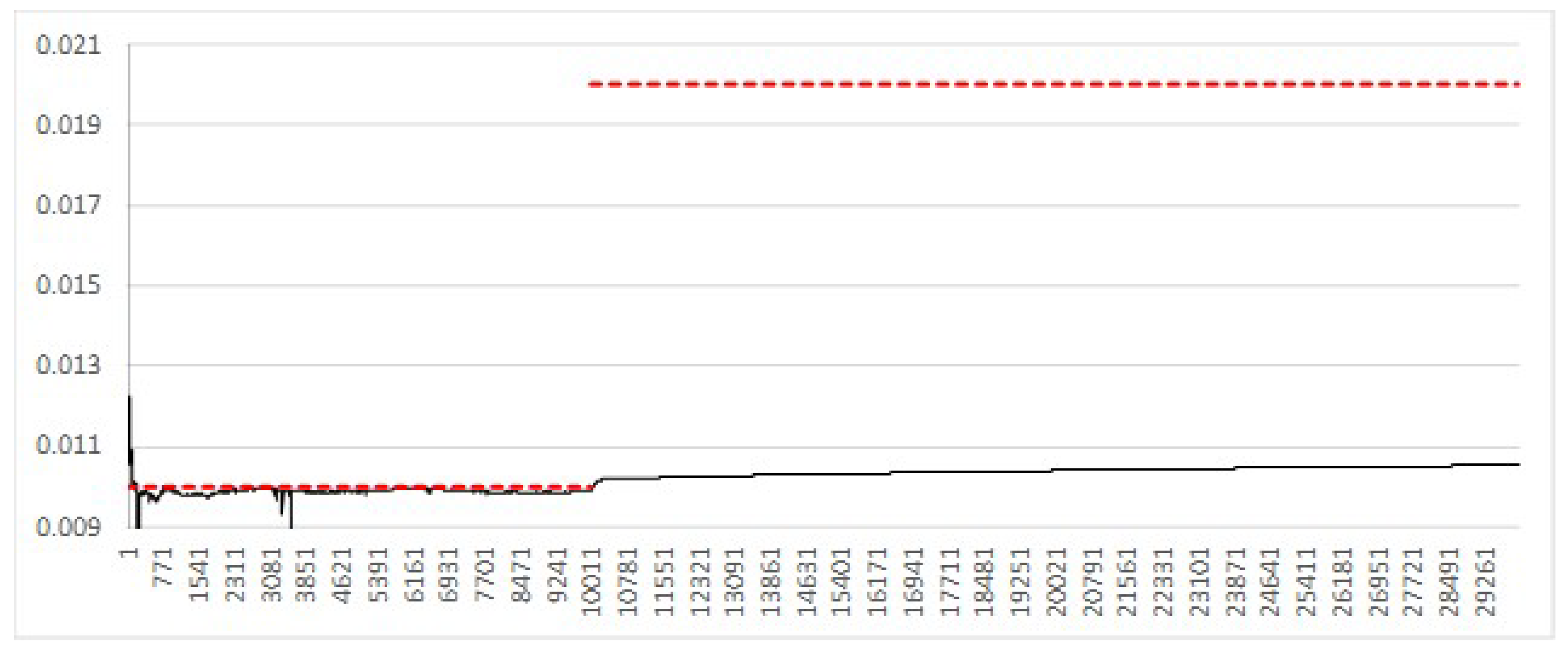
The Gaussian process as the underlying dynamic demonstrates the behaviour of the measure when the data generating process matches the assumption in the filter. As the estimated parameter posterior converges to the value of $\sigma$ used to generate the data, increasingly less perturbation is required, reflecting the correspondence between the filter assumption and underlying data. Simulation results shown in Figure 11 illustrate the convergence of $\varphi$ for different perturbation variance parameter $\gamma$. Unsurprisingly, high $\gamma$ results in noise in the convergence, highlighting the need for some implementation specific tuning of this parameter.

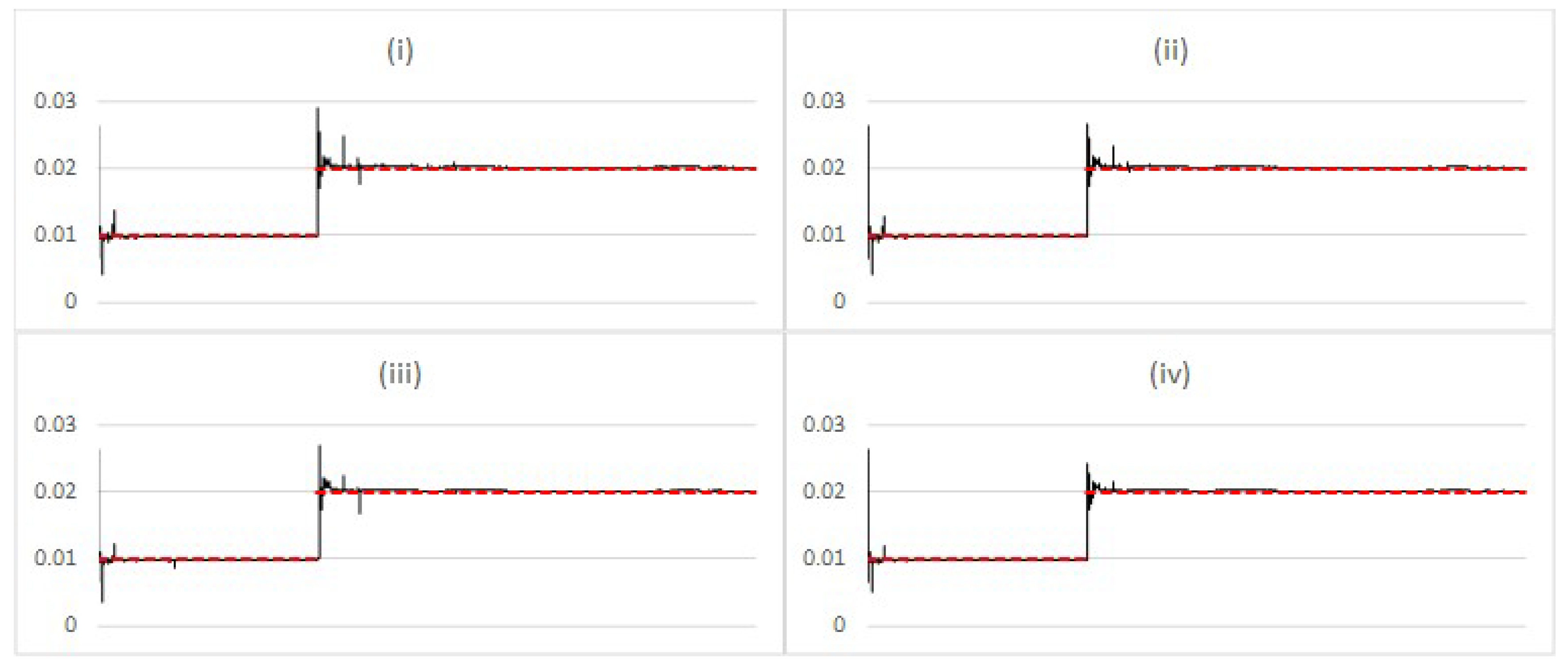
When the observations are generated by a stochastic dynamic with a regime shift in the volatility, the regime change is marked by a sharp increase in $\varphi$, reflecting sudden adaptation to the new model state. Before and after the regime change, the data-generating dynamics are Gaussian and therefore the behaviour of $\varphi$ is similar to the previous section. The rate of convergence of $\varphi$ is slower for the higher $\sigma$ following the regime change, indicating a relationship between the rate of convergence of $\varphi$ and $\sigma$. The results are shown in Figure 12 for varying levels of $\gamma$.

If the filter assumption does not match the dynamics of the underlying data, $\varphi$ will not tend to converge to zero. This becomes particularly clear in the case of stochastic volatility, where $\varphi$ tends towards a constant value reflecting the changing volatility. Figure 13 shows some examples of the behaviour of $\varphi$ for varying levels of volatility of volatility in the dynamics generating the observations, using $\gamma =0.001$ corresponding to chart (iii) in Figure 11.

4. Conclusions

By evolving a particle–specific kernel–smoothing parameter according to a genetic algorithm, we have obtained a sequential filter which is able to adapt rapidly to both stochastic volatility and volatility regime shifts. This is despite the fact that the stochastic dynamics assumed for the purpose of calculating the likelihood used in the update step of the particle filter display neither of these features. Essentially, the filter construction is agnostic about the presence of stochastic volatility and volatility regime shifts, but nevertheless the filtering output rapidly reflects these features if present. The approach illustrated here for the volatility parameter of an arithmetic Brownian motion can be applied to the fixed parameters of any baseline model, with the filtering algorithm providing a diagnostic on whether the data are consistent with constant parameters, or whether it reflects continuous or discontinuous changes in these parameters.