Abstract
The key to understanding the dynamics of stock markets, particularly the mechanisms of their changes, is in the concept of the market regime. It is regarded as a regular transition from one state to another. Although the market agenda is never the same, its functioning regime allows us to reveal the logic of its development. The article employs the concept of financial turbulence to identify hidden market regimes. These are revealed through the ratio of the components, which describe single changes of correlated risks and volatility. The combinations of typical and atypical variates of correlational and magnitude components of financial turbulence allowed four hidden regimes to be revealed. These were arranged by the degree of financial turbulence, conceptually analyzed and assessed from the perspective of their duration. The empirical data demonstrated ETF day trading profits for S&P 500 sectors, covering the period of January 1998–August 2020, as well as day trade profits of the Russian blue chips within the period of October 2006–February 2021. The results show a significant difference in regard to the market performance and volatility, which depend on hidden regimes. Both sample data groups demonstrated similar contemporaneous and lagged effects, which allows the prediction of volatility jumps in the periods following atypical correlations.
1. Introduction
The year 2020 was a real challenge for all global stock markets. The spread of the new virus, COVID-19, beyond the borders of China and the follow-up pandemic had a negative impact on the global economy and triggered a serious economic crisis. According to extensive research (Matos et al. 2021; Naidu and Ranjeeni 2021; O’Donnell et al. 2021; Seven and Yılmaz 2021), its consequences may well be compared with those during the contemporary history of economics, particularly, Black Monday of 1987, the Asian Financial Crisis of 1997, the Russian Financial Crisis of 1998, the Dotcom Bubble Crash of 2000 and, of course, the Global Financial Crisis of 2008–2010. The ex-post analysis of such events fails to answer a number of questions about how to model the dynamics of stock market performance in order, for example, to predict stock market turnarounds.
Although the reasons for such events may be different, the events themselves are assumed to reveal similar patterns and follow almost the same logic. Thus, both the participants of stock markets and the academic community seek opportunities to identify the common pattern of all crises observed in developed and emerging markets. Due to price volatility implied greater risks in trading, such as political risk, inflation rate and change or exchange rate, financial investments conducted in emerging markets are regarded as risky. However, the investors can take higher risk for obtaining higher risk premium in comparison with developed markets. What is more, fast growing potential of emerging markets contributes to the high return of financial investments. The primary focus of this research is on the S&P 500 market index measured the performance of the most capitalized companies in the most developed stock market. The secondary focus is on the main Russian equity index, the RTSI index, which measured the performance of the most capitalized companies in the emerging markets of BRIC.
In regard to this, it seems really important to develop a methodology which can help to forecast economic crises and create a system for their early prevention based on the understanding of hidden regimes (Costa and Kwon 2019; Nystrup et al. 2018). The functioning of stock markets is regarded as a sustainable regime-switching framework, involving the alternation of states. Throughout the dynamics of market performance, the regime detects comparable changes, or shifts. Thus, the regime characterizes the regular shifts rather than the particular state of the market. Although it is believed that the observed regime of any stock market follows a particular stage of the economic cycle at a point of time, it is difficult to use it as a basis for investment decisions. In this paper, we use the concept of a hidden regime with a view to describing complex dynamics of the market via the dynamics of financial turbulence. The latter is not a regular and, therefore, observable phenomenon. There are many reasons that account for such a deep interest in stock market regimes in the sphere of financial modeling. First, the idea of regime-switching framework is inherent for the market and, therefore, intuitively understandable. Hidden regimes were first mentioned in connection with the description of business cycles (Hamilton 1989). The aim was to predict recession and recognize long-term trends in business activities. Second, the modeling of the market processes across its regime enables us to consider nonlinear effects and, thus, ensure more accurate forecasting of more complicated processes.
One of the basic tools used to identify the latent changes in a market’s behavior is the Hidden Markov Model, introduced by Hamilton (1989) and Diebold et al. (1994). While Hamilton used the model with regular probabilities of switching from one state to another, Diebold assumed there could be a model with probabilities changing over the time.
At present, there are ongoing lively discussions among scholars on the subject of using the concept of hidden regimes to explain some theoretical and practical financial issues.
2. Literature Review
In regard to the former, the obtained results demonstrate the specifics of modeling and forecasting market performance and volatility. For example, Paolella et al. (2019) developed a multivariate model of financial asset returns across a switching framework, which takes into account asymmetry and heavy-tailed distribution. The use of the hidden regime concept allows more accurate predictions of risk assessment and may help develop the strategy of dynamic risks control, thus considerably reducing losses when the regime switches. Another study (van Beek et al. 2020) discussed the options of generalizing the hidden Markov model in case of self-similar processes. Liu et al. (2020) modified the GARCH model by applying the Markov switching model. The results of the study are consistent with the volatility timeline structure. The application of a regime-switching framework does not necessarily mean using the Markov models. Szulczyk and Zhang (2020) delivered another quite interesting approach towards the development of switching regression models. These are more effective in explaining the situations and phenomena in comparison with the well-known linear models with factor specifications.
In regard to the applied research issues, Nystrup et al. (2018) obtained promising results after using the hidden Markov model with time-varying parameters to forecast the numerical characteristics of the returns distribution in the framework of a dynamic approach for the evaluation of portfolio performance. The study demonstrates the effectiveness of this approach through the review of risk assets in the portfolio across the detected regime. This idea was further developed in the study by Costa and Kwon (Costa and Kwon 2019). In addition to the applied portfolio’s performance, the hidden regime concept is used in order to find arbitrage opportunities in a stock market across the dynamics of the corresponding futures market (Alemany et al. 2020).
Most of the studies mentioned above (see, among others, Chevallier and Goutte 2015; Kirkby and Nguyen 2020), consider hidden regime-switchers in the context of jump risks. However, jump risks should be regarded as a result of regime switching, revealing neither their character nor their reasons.
We assume that the change of another undiversified risk, namely, correlation risk, is what underlies the mechanism of regime switching. Thus, it is logical to conduct a further analysis in terms of correlation and its impact on financial turbulence.
At present, correlation mechanisms are widely used by economists when dealing with applied tasks in stock markets both from a static perspective (when diversifying idiosyncratic risks in non-turbulent periods of correlation consistency) and a dynamic perspective (if it is necessary to account for losses across failed diversification (Andersson et al. 2008; Engle 2002; Endovitsky et al. 2017; Endovitsky et al. 2018)). This approach was developed in the study by Page and Panariello (2018). The authors analyzed the correlations between financial tools from a dynamic perspective, thus clearly demonstrating that diversification definitely requires considering risks resulting from events which refer to the left tail of the returns distribution. This is where the portfolio performance is most sensitive. On the basis of their calculations as well as the results obtained by Baumeister and Johnson (Baumeister et al. 2001; Johnson et al. 2014), Page and Panariello showed that conditional correlations between asset classes are considerably higher for left tail returns than for right tail returns or the distribution in general. The study concludes that in order to increase the efficiency of the investment strategy, it is necessary to dynamically optimize them by the degree of downside risk.
While Page and Panariello did not consider cryptocurrencies as financial tools, the high interest in cryptocurrencies creates threats to the investment industry. Referring to Yuneline (2019), despite the discussions surrounding the nature of cryptocurrency, its legal and economic perspectives and whether it can qualify as money in a real economy, cryptocurrency may be considered as an investment asset rather than a currency. On the one hand, as an asset that is not issued by any central authorities, its values are not directly influenced by monetary policy. Corbet et al. (2018) document the increase regarding them as an investor “save heaven” or “protection asset”. On the other hand, cryptocurrency has no intrinsic value and it is not backed with any assets. Furthermore, the high price volatility and other risks may lead to the bubble panic and destroying investment value. Liu (2018) particularly focused on the influence of cryptocurrencies on portfolio diversification. Nunez (Núñez et al. 2019), however, provided a convincing argument showing that cryptocurrencies fail to maintain diversification in the case of a market crash. More recently, Foglia and Dai (2021) provided fresh evidence of the dynamic connectedness between economic policy uncertainty index (EPU; Baker et al. (2016)) and the cryptocurrency price uncertainty index. The authors found that EPUs have positive predictive power for cryptocurrency uncertainty, i.e., dictate the behavior in the cryptocurrency market. The investors who are likely to diversify their portfolio between the conventional assets or just trade in the cryptocurrency market should keep their eyes on the regular news, including economic growth, policy changes or any crises to predict dramatic price fluctuations.
The focus of this study is to develop a methodology for detecting the hidden regimes of stock markets caused by financial turbulence patterns, as well as the analysis of their impact on risk and return values.
The paper is hereafter structured as follows. Section 3 presents a consideration of the financial turbulence concept, with a focus on the methods of its calculation and decomposition into correlations and magnitudes. Section 4 describes a methodology for risk analyses and forecasting based on stock market hidden regimes, and whether the constructs of the financial turbulence demonstrate atypical patterns in comparison with the norms for a particular area. The calculations are based on the mechanism of a rolling estimation of current values of financial turbulence and its constructs for a given opportunity space. This section on approbation of the suggested approach delivers the results of a practical evaluation based on its application to the US and Russian stock markets. The practical relevance of the research lies in obtaining additional data on areas of investment from the components of financial turbulence with the help of simultaneous and lagged effects, which are typical of a market regime. These data allow us to increase the explanatory power and forecasting capacity of stock market analysis for investors. Section 5 provides the discussion of the significance of our findings. Section 6 draws the conclusions.
3. Methodology
As a rule, any discussions, including those among scholars, about the features of turbulent periods and regime switching are preceded by the “black swans” phenomenon, fraught with various financial crises (see, among others, Chow et al. 1999; Kritzman and Li 2010; Kritzman et al. 2012; Kinlaw and Turkington 2014). Each of these crises are unique in their reasons and the mechanism of development. However, all of them have one common feature, namely, the emergence and spread of abnormal trends in the market.
The identification of Chow’s turbulent periods (Chow et al. 1999) was suggested on the basis of multivariate outliers found with the Mahalonobis distance (Mahalanobis 1927; Mahalanobis 1936), and was initially applied to archaeology for the classification of human skulls:
where is a multivariate outlier at a time point ; is the vector of security asset returns for a time period ; is the vector of average historical return on assets; is the sample covariance matrix of historical asset returns.
Although the approach suggested by Chow et al. was to mainly generalize the Markowitz portfolio theory and observe various stock market regimes with a view to improving its sustainability, on the whole, it was the Mahalanobis distance concept that became the basis for developing special measures for measuring financial turbulence in a market.
The financial turbulence concept is well-developed in the paper by Kritzman and Li (2010), published almost 10 years later and following yet another financial crisis. The authors linked financial turbulence with the level of deviations in the complex multivariate system of the stock market. They developed a special system of measures to be used in a particular opportunity space for assessing the level of correlations and, thus, the investment capacity. According to Kritzman and Li, this would help to identify the deviation periods in which the patterns of security assets behave uncharacteristically. As a result, asset prices may fluctuate dramatically, thus weakening the correlations among some assets and strengthening them among others.
In order to measure financial turbulence, the Mahalanobis distance should be averaged by the number of assets allocated in a particular opportunity space:
where is the financial turbulence at a particular time point ; is the the number of assets in a particular investment opportunity space.
The obtained variate can be regarded as a measure of uncharacteristic asset behavior at the considered time point in regard to the preceding historical perspective. In other words, it is the measure of deviation at a particular time point.
It is important to distinguish financial turbulence from cross-sectional volatility, which measures the average cross-sectional dispersion of stocks returns (see, among others, Bali et al. 2011; Fu 2009). However, it fails to consider the average return on particular assets. Moreover, turbulence differs from the rolling volatility of a portfolio of stocks (see, among others, McMillan and Speight 2004; Fouque et al. 2017). This difference comes from the fact that turbulence describes deviations at a particular time point rather than the volatility of a portfolio of stocks over an extended period.
Kinlaw and Turkington (2014) extended the idea of Kritzman and Li (2010) and suggested a method for the decomposition of financial turbulence into correlations and magnitudes. The correlation components give a general description of the correlations in a particular investment opportunity space and shows how the correlations change over a historical period of time, i.e., the changes in market correlation risks.
The correlational component of financial turbulence is identified through the factorization of the “full-scale” financial turbulence into magnitude components:
where is the magnitude contribution for a time period ; is the random diagonal asset dispersion matrix from a historical perspective.
As follows from the expression (4) above, is a mean of standard asset returns for a particular time point. It only shows whether the deviation of asset returns for this time period is large or small relative to their historical means, i.e., it captures the extent of the price movement. By using the empirical distribution of , we can identify the time periods of atypical magnitude, which is more appropriate to regard as a jump risk. Financial instruments demonstrate magnitude surprise at periods when the observed values of are more to the right of the upper unilateral quantile of level of distribution:
The quantile is set exogenously.
We can observe the events with , called “correlation surprise”, when security assets demonstrate atypical correlations, i.e., correlations between some assets are weaker and between other assets are stronger. The episodes with (absence of “correlation surprise”) prove the correlations typical. Such an approach seems convenient for, at least, two reasons. Firstly, it summarizes and unifies the general atypicality of correlational interactions over a period of time in any investment opportunity space. Secondly, when calculating the correlation surprise, we focus not on whether the correlation is high or low but rather on its deviation from historical norms, whatever they were. It is by this that we detect changes in market correlation risks.
To develop intuition around the concept of correlation surprise, let us consider a single asset with an expected zero-beta return and finite variance . The turbulence of this asset is a squared standard value of its return:
Since the correlation coefficient for one asset is, by definition, equal to 1, the correlation surprise will equal precisely the financial turbulence.
If we consider two assets with zero-beta, it is easy to show that the financial turbulence is also a standardized variable:
Thus, the correlation in the financial turbulence of the two assets will look as follows:
The expression (7) demonstrates that the correlation contribution in the financial turbulence is a functional derivative only from the correlation coefficient and standard values of asset returns, i.e., values which are factorized in relation to volatility. Thus, the correlation surprise contains information not about risks but about how coordinated the price movement is in a given space.
If the asset returns are orthogonal (), the correlation surprise is equal to one, which means we should not expect any movement. If correlation interaction grows in a particular investment space, investors regard it as typical, and in this case the correlation value will be less than one. By contrast, in the case of a large correlational deviation, correlation will become increasingly atypical. It is possible to observe it through the values of correlation surprise as they will exceed one and, thus, increase the degree of market correlation risk.
Following these considerations, we can correlate the observed actual state of the market with one of the four hidden regimes from the perspective of whether there are any atypical patterns in the constructs of financial turbulence:
- The regime of full-scale financial turbulence. This is identified through atypical values of its two components. Deviations responsible for such a regime demonstrate the anticipated exposure to increasing risk. As the market correlational risks grow, asset returns among previously uncorrelated instruments may become positive, thus making the diversification effects shrink to zero. After a regime-switch, the lagged volatility grows and achieves an all-time high. During such periods, returns are low or even negative, which is why this regime may precede downward trends. Typically, this regime in the stock market accounts for about 5–8% of all regimes, which enables us to assume that it is due to the crisis phenomena (which are rare events). We also assume that during such periods, the developing markets can experience capital outflow, while the developed markets are able to control this process and ensure the outflow of capital into safe assets.
- The regime of financial turbulence across atypical correlations. This is highly frequent and accounts for 55–60% of all regimes. The changes in correlational risks revealed through atypical values of correlations in the financial turbulence do not largely affect the market exposure to the systemic risks. In such a regime, we can observe low values of both returns and volatility. The price performance is connected with low return magnitudes around means, which resembles some kind of random volatility. The absence of significant changes in asset prices allows the effective use of a portfolio optimization in risk management.
- The regime of financial turbulence across atypical magnitude. This is characterized by atypical price performance. The market correlational risks do not exceed the historical norms, and the asset returns change insignificantly, thus making the diversification effective in idiosyncratic risks management. Such dynamics fill market participants with optimism and make the risk premium higher. During such a regime, the market demonstrates the highest asset returns in contrast with the other regimes. Although the returns deviate from their historical means, they remain positive, thus showing the anticipation of upward trends. Usually, it accounts for 10–15% of all regimes.
- The regime with laminar conditions. It is characterized by the absolute absence of any abnormalities in the financial turbulence structure and fits within its historical means. In such a regime, the market, as a rule, follows regular patterns because the price movement is not strong enough to produce deviations. Alternatively, such a regime can be characterized as the situation of anticipation before changes start. Usually, it accounts for 17–30% of all regimes.
Let us examine the features of the above-mentioned stock market regimes. This research is based on two groups of data describing an attractive investment space, which corresponds to ETFs for the S&P 500 index and the blue-chip space, included in the RTSI index (Table 1).

Table 1.
Description of source data.
We made experimental calculations for both groups of investment options. The experiments included the following stages:
- Calculations of historical means of financial turbulence.
- Decomposition of financial turbulence into correlations and magnitudes, and calculation of their historical distribution.
- Division of observations of a sample into two groups:
- Showing atypical magnitude, i.e., located more to the right of the 20% upper (unilateral) quantile:
- Showing typical magnitude, i.e., located more to the left of the 20% upper (unilateral) quantile:
- Division of observations of a sample into two groups:
- Showing atypical correlations ();
- Showing typical correlations ();
- Formation of samples which correspond to the above-mentioned market regimes at the cross point of the two independent universes.
- Analysis of contemporaneous and lagged effects, determined by the hidden market regimes.
4. Results
4.1. Analysis of the Dynamics with Hidden Market Regimes
Consistent with the logic of our methodology, we computed the values of financial turbulence and its unobservable components for both groups of investment options, as shown in Figure 1. The charts show the effects of clustered values of financial turbulence and its magnitude components. The clusters with high values demonstrate the most turbulent periods in the stock market. The dynamics of correlation components is not so highly clustered. Thus, it is consistent with the assumption that both components are orthogonal, i.e., they demonstrate different information about the contemporaneous market regime.
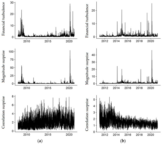
Figure 1.
Financial turbulence and its components for spaces of the (a) S&P 500 index and (b) RTSI index.
To identify the hidden regimes, we use two independent period groupings by the observable values of financial turbulence components. As a result, we have four samples, whose sizes are presented in Table 2. The first value in brackets refers to the space of the S&P 500 index and the second value refers to the space of the RTSI index. The ratios of the regimes, as we see, do not differ much.
Table 2.
The number of observations in the regime-based samples.
The examination of the features of hidden market regimes is based on the four respective groups of observations.
Let us consider the contemporaneous effects resulting from atypical magnitudes and atypical correlations, i.e., the effects within the full-scale financial turbulence and financial turbulence with atypical magnitude. Table 3 demonstrates the magnitude means for the considered samples. Interestingly, the samples with correlation surprise, on average, demonstrate a lower magnitude value than those without correlation surprise. This empirical evidence confirms that when volatility is high, we can observe typical correlation rather than atypical. The detected differences between the samples and, therefore, regimes have a statistical relevance.
Table 3.
Conditional mean value of risk on days with atypical magnitude.
Table 4 presents an analysis of the lagged effects in the magnitude dynamics over the full-scale regime of financial turbulence and financial turbulence across atypical magnitude. The calculations provide evidence that for each of the investment opportunity options, days with the highest atypical magnitude are preceded by days with atypical correlation. Consequently, it gives evidence that volatility coupled with an atypical correlation can be regarded as having a highly probable volatility prediction for the following day. The Kruskal–Wallis non-parametric test statistic and the respective p-value reveal significant differences in the observed magnitude values within samples with correlation surprise and without it for ETF space of S&P 500 sector indices. It was also found that RTSI equities demonstrate higher risk values, if preceded by an atypical correlation. This difference is of statistical relevance as well.
Table 4.
Conditional mean value of risk on days following the days with atypical risks.
The given result provides evidence that the volatility of a coming period is substantially different across the regime-based groups in the market.
It is obvious that investment decisions are often based on the evaluation of future returns. Now, using the above-mentioned samples for the two investment opportunity options (S&P 500 sector ETFs and RTSI equities), let us examine how market hidden regimes can affect the characteristics of a coming period. Table 5 and Table 6 demonstrate the results of asset return calculations for S&P 500 and RTSI indices, the number of days with positive returns as well as the total number of observations for each sample. The credibility of the research findings about the differences between the hidden market regimes, revealed through risks and returns characteristics, is also confirmed by a pair-wise consistency check and is given in Table 7 and Table 8. In these tables, the above-diagonal space contains Student’s t test statistics about the equality of the sample means, while the under-diagonal space contains Bartlett test statistics about the equality of sample dispersions. It is possible to state that almost all the regimes under consideration differ from one another in at least one statistical criterion.
Table 5.
Daily asset returns distribution for the S&P 500.
Table 6.
Daily asset returns distribution for the RTSI index.
Table 7.
Pair-wise consistency check of hidden regime features for the S&P 500 (the p-value is given in brackets).
Table 8.
Pair-wise consistency check of hidden regime features for the RTSI (the p-value is given in brackets).
The differences between the market regimes, as given above, provide evidence that the values of the investment characteristics have a conditional character and are affected by the processes, or regime, “observed” on the previous day. Thus, we managed to provide convincing empirical proof of the existence of contemporaneous and lagged effects in risks and returns across the financial turbulence components which affect the regime pattern.
The main benefits of hidden market regimes are contemporaneous and lagged effects in risks and returns across the financial turbulence components affected by the regime pattern. It is attractive for investment strategy development, and it would be rather hard to only use these regimes. As will be seen in the next section, hidden market regime switching based on components of financial turbulence occurs more often than Markov regime switching. Markov regimes are more sustainable over time and switch less frequently due to slow reflection of available information.
The empirical analysis below shows the relationship between our hidden market regimes and subsequent Markov regimes. The estimated parameters of the S&P 500 index for a four-regime Markov switching model obtained with the maximum likelihood method are reported in Table 9. When the market moves from regime 0 to regime 3, the estimated mean parameter decreases, while the estimated standard deviation parameter increases. From these arguments, our four regimes (0, 1, 2 and 3) have meaningful interpretations as the tranquil, volatile, turbulent or panic regimes, respectively. It is also evident that all estimated probabilities of permanence in a given regime, i.e., diagonal values of estimated transition probabilities matrix, are larger than 92%.
Table 9.
Four-regime Markov switching models: estimated parameters for the S&P 500 index returns (years 1999–2020). AIC and BIC are the Akaike and Bayesian Information Criterion, respectively.
We used smoothed probabilities to determine whether a given day belongs to the tranquil, volatile, turbulent or panic regimes. In Figure 2, we plot the identified Markov regimes. In Table 10, we report the percentage of time spent by the S&P 500 index in each one of the four considered regimes when considering the whole period (1999–2020) and the COVID-19 pandemic period (2020). During 2020, the turbulent regime is the most frequent, and the panic regime is observed three times more often than the entire period of 1999–2020.
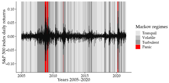
Figure 2.
Time-series plots for the S&P 500 returns and different regimes based on smoothed probabilities.
Table 10.
Percentage of time spent by the S&P 500 index in each regime.
In Table 11, we report the annualized mean returns and volatility for the S&P 500 index during Markov regime switching days to evaluate the relationship between hidden market regimes and subsequent Markov regimes. The average daily S&P 500 return on the days with Markov regime switching following laminar hidden regime was 0.7039, and the standard deviation 0.1261. In contrast, the days characterized by atypical volatility or correlation tended to exhibit negative average returns while Markov regime switching. Table 11 shows that the average return is lower and the standard deviation of returns is higher following any atypical patterns in the constructs of financial turbulence. Finally, Table 11 reveals that the percent of the days with positive returns is lowest following days characterized by full-scale turbulence regime.
Table 11.
Daily returns distribution for the S&P 500 during switches among four Markov regimes.
Next, we consider RTSI index in the same matter. Table 12 reports the estimated parameters for the returns of the RTSI index for the period of January 2005 to December 2020. As in the former case, we identified four regimes for the RTSI index returns representative of the tranquil, volatile, turbulent and panic states. In this case, the probability of permanence in each regime is no less than 92.1%. Transition probabilities matrix is close to the previous case. The percentage of time spent by the RTSI index in each regime reported in Table 13 is quite different from S&P 500 index. In particular, the most frequent regime is the volatile one during the first months of the COVID-19 crisis.
Table 12.
Four-regime Markov switching models: estimated parameters for the RTSI index returns (years 2005–2020). AIC and BIC are the Akaike and Bayesian Information Criterion, respectively.
Table 13.
Percentage of time spent by the RTSI index in each regime.
Figure 3 plots the different regimes based on smoothed probabilities, together with the time series plots, for the RTSI index.
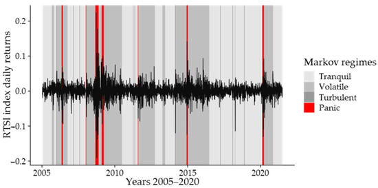
Figure 3.
Time-series plots for the RTSI index returns and different regimes based on smoothed probabilities.
In Table 14, we report the annualized mean returns and volatility for the RTSI index during Markov regime switching days to evaluate the relationship between hidden market regimes and subsequent Markov regimes. As in the S&P 500 index, the average return is lower and the standard deviation of returns is higher following any atypical patterns in the constructs of financial turbulence. Table 14 shows that the average daily RTSI return on the days with Markov regime switching following only laminar hidden regime was positive (0.5731), and the standard deviation was minimal (0.2361).
Table 14.
Daily returns distribution for the RTSI during switches among four Markov regimes.
4.2. Robustness Check
In this section, we provide an analysis of robustness of the proposed approach and, with this aim, we consider two sub-samples of the period of COVID-19. Performing the same regime switching analysis, we do not find any evidence that our hidden market regimes insignificantly influence S&P 500 (Table 15). In Table 16, we apply our analysis to the RTSI index. We find consistent results across both indices. Captured empirical regularity of asset returns and volatility reveals that the Markov regime switching following laminar hidden regime days is characterized by both high positive average return and low volatility.
Table 15.
Daily returns distribution for the S&P 500 index during switches among four Markov regimes in the COVID-19 crisis.
Table 16.
Daily returns distribution for the RTSI index during switches among four Markov regimes in the COVID-19 crisis.
These results suggest that our hidden market regimes contain incremental information about future return and volatility. Our four hidden market regimes, from the perspective of whether there are any atypical patterns in the constructs of financial turbulence, are useful candidates to devise an early warning system that is able to anticipate highly fluctuating Markov regime switching.
4.3. The Analysis of Market Hidden Regimes in Modern History
It seems important to turn now to some episodes and details in modern history. It will help to appreciate the practical implications of understanding the impact that hidden regimes, the full-scale regime in particular, have produced on stock market. One of the most striking examples of full-scale turbulence was the stock market crash in 2008, caused by liquidity failures of major US banks in the context of the preceding subprime mortgage crisis. Figure 4 demonstrates the stock market diagram for the S&P 500 index’s performance as well as the components of financial turbulence observed in the autumn of 2008. The horizontal lines in the charts mark the threshold values. If exceeded, they signal the occurrence of correlation surprise or magnitude surprise, respectively, or, in other words, full-scale financial turbulence.
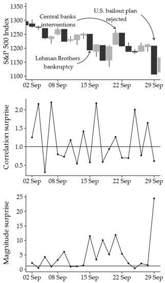
Figure 4.
Analysis of the financial turbulence, September 2008.
Within the considered timeline, the surprise correlation exceeded one nine times as much: it was observed on the 2nd, 3rd, 5th, 10th, 12th, 16th, 19th, 24th and 26th of September. Interestingly, the day Lehman Brothers, the biggest bank in US history, declared bankruptcy was preceded both by atypical correlation and atypical magnitude. On the very day of the officially declared bankruptcy, the 15th of September, the correlation surprise did not exceed 1. However, there was a volatility jump, reflected in the magnitude surprise on that day.
The average daily mean of the magnitude surprise for the days following a correlation surprise was 6.78, and the mean of the S&P 500 index’s performance reached 3.36%. By contrast, the average daily mean of the magnitude surprise for the days following periods without correlation surprise was 3.55, and the mean of the S&P 500 index’s performance reached 0.71%.
The biggest loss was observed on 29 September and reached 8.81%. The magnitude surprise on this particular day reached its all high—24.48. On the eve of this event, the correlation surprise was 1.65, but on 29 September, it struggled to reach 0.61.
The charts illustrate that the correlation surprise lasted for nine trading days. Thus, in the considered month, it is possible to observe not only atypical volatility, but also underlying changes in the asset correlation affected by the hidden regimes.
Let us consider another episode in the history of financial turbulence, namely, the US stock market crash in 2018 (Figure 5). In light of negative investment expectations resulting from monetary policy mistake by the Federal Reserve, rising interest rates, large amount of uncertainty in the global economy and tariffs on imported goods policy introduced by the Trump administration (Burggraf et al. 2020), the S&P 500 index lost almost 4% on just one day, the 10th of October. The crash was preceded by atypical correlation and magnitude, which are characteristics of full-scale financial turbulence. On the day before the crash, the correlation surprise reached almost its record of 4.19, but on the day of the crash, the 10th of October, it struggled to reach 0.45. The magnitude surprise changed its value from 0.64 on the day before the crash and became 7.71 on the day of the crash.
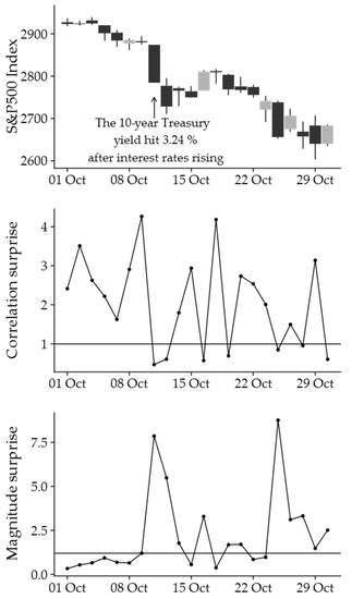
Figure 5.
Analysis of the financial turbulence, October 2018.
Finally, let us consider a third episode which relates to the market crash in the spring of 2020 (Figure 6). Atypical correlation and magnitude could be observed on the 26th of February. This was followed by a volatility jump the next day and the resulting loss reached 4.41%, according to the S&P 500 index. It was the most dramatic drop since September 2008. On the 6th of March atypical correlation and almost atypical risk was observed. The next day, losses reached 7.60%, according to the S&P 500 index.
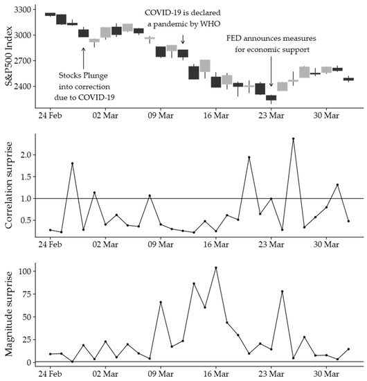
Figure 6.
Analysis of the financial turbulence, February–March 2020.
Next, on the 18th of March, many logically expected that the market had reached its minimum, and therefore, there was very little chance of sinking further as the correlation surprise did not exceed 1 and the magnitude surprise, though high, demonstrated a downward trend. However, on the 19th of March, both the correlation surprise and magnitude surprise showed high values, which meant there was an approaching period of financial turbulence. Over the next two days, the losses reached 6%, according to the S&P 500 index.
Now we will consider the first six months of 2020 for the Russia Stock Market. On the 20th–21st of January, the market experienced both atypical correlation surprise and magnitude, which provided evidence of full-scale financial turbulence (Figure 7a). These dates were then followed by sharp risk jumps and the index price dropped for four trading days in a row. The magnitude was highest on the fourth day (27th of January). The total loss over that period was slightly under 5%, according to the RTSI index.
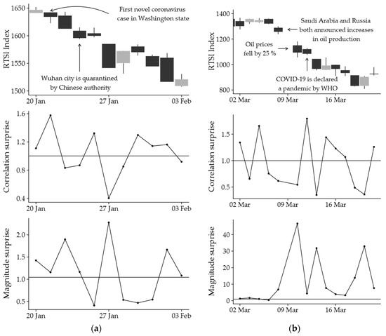
Figure 7.
Analysis of the financial turbulence: (a) January–February, (b) March 2020.
The next sharp drop caused by full-scale financial turbulence occurred on the 4th of March (Figure 7b). The magnitude slightly exceeded the threshold value. Over the next five trading days, the RTSI index decreased by almost 40% and the magnitude surprise on the 10th of March showed one of its records of 46.68.
5. Discussion
The conducted research contributes to the global knowledge pool, at minimum, in three aspects.
First, we suggest our own classification of the stock market hidden regimes. The examined regimes were given a consistent consideration and interpretation. We also used statistical tests to compare and contrast the stock market features within different regimes. The article provides the analysis of some episodes of regime switching occurring in financial history. The results obtained across the S&P 500 sample are consistent with the research conducted by many analysts (Ang and Timmermann 2012; Kinlaw and Turkington 2014). Armstrong and Bradfield (2015) revealed similar effects across African stock markets. This paper provides the data on regime switching patterns detected on the Russian stock market with reference to the events which took place in 2020.
Second, we propose a methodology to detect hidden market regimes. The methodology is based on capturing single changes in the degree of non-diversifiable orthogonal components of financial turbulence that describe correlation and jump risks. This study extends and summarizes the results of research into hidden market regimes in terms of correlation (Kritzman and Li 2010; Kinlaw and Turkington 2014) and volatility jumps (Chevallier and Goutte 2015; Kirkby and Nguyen 2020). The insight into the intrinsic features of the hidden market regimes provides fuller evidence about their characters and the reasons for behavioral patterns.
Third, we describe the impact that hidden market regimes have on asset risks and returns. The obtained results can be used to develop strategies for a turbulence-resistant investment portfolio with reference to the type of market regime (Page and Panariello 2018; Nystrup et al. 2018; Paolella et al. 2019), the systems of early predictive capacity (Golub et al. 2018; Liu et al. 2020) and also in exploring the patterns and dependency of different sectors of a financial market (Alemany et al. 2020).
6. Conclusions
It is obvious that stock markets are constantly developing, changing and updating themselves. This refers not only to institutional aspects but, first of all, to statistic aspects. Although unobservable, the latter aspects have quite tangible effects on the performance of assets and investment opportunities. Thus, their detection requires a specially designed methodology.
In this article, we provide a developed classification of hidden market regimes as well as providing a proper consideration of these from the perspective of contemporaneous and lagged effects, which affect the investment characteristics of financial instruments. In order to detect a hidden market regime, it is necessary to decompose the financial turbulence into correlation and magnitude components. The magnitude allows detecting atypical values of returns volatility in relation to their history. Correlations, irrespective of magnitudes, show the degree of atypical assets interaction over a time period. In other words, they show a risk correlation baseline in the stock market.
The research finds that the detection of a stock market regime provides additional evidence for future changes of assets performance. The particular examples of the stock markets in the US and Russia, both conceptually and empirically, show that these data have a predictive capacity to forecast volatility jumps over time periods following atypical correlations. The study also demonstrates that the considered hidden regimes have at least one different statistic criterion, i.e., that of returns or volatility.
The suggested methodology has a number of important empirical applications. If taken into consideration, a hidden regime pattern can ensure a proper decision-making model and, thus, improve the efficiency of asset risk algorithms.
Obviously, a number of issues are yet to be addressed. First, it is necessary to explore the clustering of the effects, resulting from regime switches. Second, it is important to investigate methods for forecasting the duration of the detected contemporaneous and lagged effects during a regime switch. Finally, it seems productive to analyze the character of transition from one regime to another with a view to detecting regular or correctly anticipated patterns.
Author Contributions
All authors contributed equally. All authors have read and agreed to the published version of the manuscript.
Funding
This research received no external funding.
Data Availability Statement
The data are available on request from the corresponding author.
Conflicts of Interest
The authors declare no conflict of interest.
References
- Alemany, Nuria, Vicent Aragó, and Enrique Salvador. 2020. Lead-Lag Relationship between Spot and Futures Stock Indexes: Intraday Data and Regime-Switching Models. International Review of Economics & Finance 68: 269–80. [Google Scholar] [CrossRef]
- Andersson, Magnus, Elizaveta Krylova, and Sami Vähämaa. 2008. Why Does the Correlation between Stock and Bond Returns Vary over Time? Applied Financial Economics 18: 139–51. [Google Scholar] [CrossRef]
- Ang, Andrew, and Allan Timmermann. 2012. Regime Changes and Financial Markets. Annual Review of Financial Economics 4: 313–37. [Google Scholar] [CrossRef]
- Armstrong, Joanne, and David Bradfield. 2015. Correlation Surprise: The African and South African Case. African Finance Journal 17: 55–83. [Google Scholar]
- Baker, Scott R., Nicholas Bloom, and Steven J. Davis. 2016. Measuring economic policy uncertainty. The Quarterly Journal of Economics 131: 1593–636. [Google Scholar] [CrossRef]
- Bali, Turan G., Nusret Cakici, and Robert F. Whitelaw. 2011. Maxing out: Stocks as Lotteries and the Cross-Section of Expected Returns. Journal of Financial Economics 99: 427–46. [Google Scholar] [CrossRef]
- Baumeister, Roy F., Ellen Bratslavsky, Catrin Finkenauer, and Kathleen D. Vohs. 2001. Bad Is Stronger than Good. Review of General Psychology 5: 323–70. [Google Scholar] [CrossRef]
- Van Beek, Misha, Michel Mandjes, Peter Spreij, and Erik Winands. 2020. Regime Switching Affine Processes with Applications to Finance. Finance and Stochastics 24: 309–33. [Google Scholar] [CrossRef]
- Burggraf, Tobias, Ralf Fendel, and Toan Luu Duc Huynh. 2020. Political news and stock prices: Evidence from Trump’s trade war. Applied Economics Letters 27: 1485–88. [Google Scholar] [CrossRef]
- Chevallier, Julien, and Stéphane Goutte. 2015. Detecting Jumps and Regime Switches in International Stock Markets Returns. Applied Economics Letters 22: 1011–19. [Google Scholar] [CrossRef][Green Version]
- Chow, George, Eric Jacquier, Mark Kritzman, and Kenneth Lowry. 1999. Optimal Portfolios in Good Times and Bad. Financial Analysts Journal 55: 65–73. [Google Scholar] [CrossRef]
- Corbet, Shaen, Andrew Meegan, Charles Larkin, Brian Lucey, and Larisa Yarovaya. 2018. Exploring the Dynamic Relationships between Cryptocurrencies and Other Financial Assets. Economics Letters 165: 28–34. [Google Scholar] [CrossRef]
- Costa, Giorgio, and Roy H. Kwon. 2019. Risk Parity Portfolio Optimization under a Markov Regime-Switching Framework. Quantitative Finance 19: 453–71. [Google Scholar] [CrossRef]
- Diebold, Francis X., Joon-Haeng Lee, and Gretchen C. Weinbach. 1993. Regime Switching with Time-Varying Transition Probabilities. Working Paper. Philadelphia, PA, USA: Federal Reserve Bank of Philadelphia, vol. 93, pp. 283–302. [Google Scholar]
- Endovitsky, Dmitry Aleksandrovich, Valery Vladimirovich Davnis, and Viacheslav Vladimirovich Korotkikh. 2017. On Two Hypotheses in Economic Analysis of Stochastic Processes. Journal of Advanced Research in Law and Economics 8: 2391–98. [Google Scholar] [CrossRef]
- Endovitsky, Dmitry Aleksandrovich, Valery Vladimirovich Davnis, and Viacheslav Vladimirovich Korotkikh. 2018. Adaptive Trend Decomposition Method in Financial Time Series Analysis. The Journal of Social Sciences Research SPI3: 104–9. [Google Scholar] [CrossRef]
- Engle, Robert. 2002. Dynamic Conditional Correlation. Journal of Business & Economic Statistics 20: 339–50. [Google Scholar] [CrossRef]
- Foglia, Matteo, and Peng-Fei Dai. 2021. “Ubiquitous uncertainties”: Spillovers across economic policy uncertainty and cryptocurrency uncertainty indices. Journal of Asian Business and Economic Studies. [Google Scholar] [CrossRef]
- Fouque, Jean-Pierre, Ronnie Sircar, and Thaleia Zariphopoulou. 2017. Portfolio Optimization and Stochastic Volatility Asymptotics. Mathematical Finance 27: 704–45. [Google Scholar] [CrossRef]
- Fu, Fangjian. 2009. Idiosyncratic Risk and the Cross-Section of Expected Stock Returns. Journal of Financial Economics 91: 24–37. [Google Scholar] [CrossRef]
- Golub, Bennett, David Greenberg, and Ronald Ratcliffe. 2018. Market-Driven Scenarios: An Approach for Plausible Scenario Construction. The Journal of Portfolio Management 44: 6–20. [Google Scholar] [CrossRef]
- Hamilton, James D. 1989. A New Approach to the Economic Analysis of Nonstationary Time Series and the Business Cycle. Econometrica 57: 357–84. [Google Scholar] [CrossRef]
- Johnson, Nicholas, Vasant Naik, Sébastien Page, Niels Pedersen, and Steve Sapra. 2014. The Stock–Bond Correlation. Journal of Investment Strategies 4: 3–18. [Google Scholar] [CrossRef][Green Version]
- Kinlaw, Will, and David Turkington. 2014. Correlation Surprise. Journal of Asset Management 14: 385–99. [Google Scholar] [CrossRef]
- Kirkby, J. Lars, and Duy Nguyen. 2020. Efficient Asian Option Pricing under Regime Switching Jump Diffusions and Stochastic Volatility Models. Annals of Finance 16: 307–51. [Google Scholar] [CrossRef]
- Kritzman, Mark, and Yuanzhen Li. 2010. Skulls, Financial Turbulence, and Risk Management. Financial Analysts Journal 66: 30–41. [Google Scholar] [CrossRef]
- Kritzman, Mark, Sébastien Page, and David Turkington. 2012. Regime Shifts: Implications for Dynamic Strategies (Corrected). Financial Analysts Journal 68: 22–39. [Google Scholar] [CrossRef]
- Liu, Weiyi. 2018. Portfolio Diversification across Cryptocurrencies. Finance Research Letters 29: 200–205. [Google Scholar] [CrossRef]
- Liu, Yue, Huaping Sun, Jijian Zhang, and Farhad Taghizadeh-Hesary. 2020. Detection of Volatility Regime-Switching for Crude Oil Price Modeling and Forecasting. Resources Policy 69: 101669. [Google Scholar] [CrossRef]
- Mahalanobis, P. Chandra. 1927. Analysis of Race-Mixture in Bengal. Journal of the Asiatic Society of Ben-Gal 23: 301–33. [Google Scholar]
- Mahalanobis, Prasanta Chandra. 1936. On the Generalized Distance in Statistics. Proceedings of the National In-Stitute of Sciences of India 2: 49–55. [Google Scholar]
- Matos, Paulo, Antonio Costa, and Cristiano da Silva. 2021. COVID-19, Stock Market and Sectoral Contagion in US: A Time-Frequency Analysis. Research in International Business and Finance 57: 101400. [Google Scholar] [CrossRef]
- McMillan, David G., and Alan E. H. Speight. 2004. Daily Volatility Forecasts: Reassessing the Performance of GARCH Models. Journal of Forecasting 23: 449–60. [Google Scholar] [CrossRef]
- Naidu, Dharmendra, and Kumari Ranjeeni. 2021. Effect of Coronavirus Fear on the Performance of Australian Stock Returns: Evidence from an Event Study. Pacific-Basin Finance Journal 66: 101520. [Google Scholar] [CrossRef]
- Núñez, José Antonio, Mario I. Contreras-Valdez, and Carlos A. Franco-Ruiz. 2019. Statistical Analysis of Bitcoin during Explosive Behavior Periods. PLoS ONE 14: e0213919. [Google Scholar] [CrossRef] [PubMed]
- Nystrup, Peter, Henrik Madsen, and Erik Lindström. 2018. Dynamic Portfolio Optimization across Hidden Market Regimes. Quantitative Finance 18: 83–95. [Google Scholar] [CrossRef]
- O’Donnell, Niall, Darren Shannon, and Barry Sheehan. 2021. Immune or At-Risk? Stock Markets and the Significance of the COVID-19 Pandemic. Journal of Behavioral and Experimental Finance 30: 100477. [Google Scholar] [CrossRef] [PubMed]
- Page, Sébastien, and Robert A. Panariello. 2018. When Diversification Fails. Financial Analysts Journal 74: 19–32. [Google Scholar] [CrossRef]
- Paolella, Marc S., Paweł Polak, and Patrick S. Walker. 2019. Regime Switching Dynamic Correlations for Asymmetric and Fat-Tailed Conditional Returns. Journal of Econometrics 213: 493–515. [Google Scholar] [CrossRef]
- Seven, Ünal, and Fatih Yılmaz. 2021. World Equity Markets and COVID-19: Immediate Response and Recovery Prospects. Research in International Business and Finance 56: 101349. [Google Scholar] [CrossRef]
- Szulczyk, Kenneth R., and Changyong Zhang. 2020. Switching-Regime Regression for Modeling and Predicting a Stock Market Return. Empirical Economics 59: 2385–403. [Google Scholar] [CrossRef]
- Yuneline, Mirza Hedismarlina. 2019. Analysis of cryptocurrency’s characteristics in four perspectives. Journal of Asian Business and Economic Studies 26: 206–19. [Google Scholar] [CrossRef]
Publisher’s Note: MDPI stays neutral with regard to jurisdictional claims in published maps and institutional affiliations. |
© 2021 by the authors. Licensee MDPI, Basel, Switzerland. This article is an open access article distributed under the terms and conditions of the Creative Commons Attribution (CC BY) license (https://creativecommons.org/licenses/by/4.0/).