Article

Numerical Algorithms for Reflected Anticipated Backward Stochastic Differential Equations with Two Obstacles and Default Risk

1
Department of Mathematics, University of Kaiserslautern, 67663 Kaiserslautern, Germany
2
Department of Mathematics, University of Kaiserslautern, Fraunhofer ITWM, 67663 Kaiserslautern, Germany
*
Author to whom correspondence should be addressed.
Risks 2020, 8(3), 72; https://doi.org/10.3390/risks8030072
Submission received: 27 April 2020 / Revised: 11 June 2020 / Accepted: 12 June 2020 / Published: 1 July 2020
(This article belongs to the Special Issue Computational Finance and Risk Analysis in Insurance)

Abstract

:
We study numerical algorithms for reflected anticipated backward stochastic differential equations (RABSDEs) driven by a Brownian motion and a mutually independent martingale in a defaultable setting. The generator of a RABSDE includes the present and future values of the solution. We introduce two main algorithms, a discrete penalization scheme and a discrete reflected scheme basing on a random walk approximation of the Brownian motion as well as a discrete approximation of the default martingale, and we study these two methods in both the implicit and explicit versions respectively. We give the convergence results of the algorithms, provide a numerical example and an application in American game options in order to illustrate the performance of the algorithms.

1. Introduction

The backward stochastic differential equation (BSDE) theory plays a significant role in financial modeling. Given a probability space ( Ω , F , P ) , where B : = ( B t ) t 0 is a d-dimensional standard Brownian motion, F : = ( F t ) t 0 is the associated natural filtration of B, F t = σ ( B s ; 0 s t ) , and F 0 contains all P-null sets of F . We first consider the following form of BSDE with the generator f and the terminal value ξ :
Y t = ξ + t T f ( s , Y s , Z s ) d s t T Z s d B s , t [ 0 , T ] .
The setting of this problem is to find a pair of F t -adapted processes ( Y , Z ) S F 2 ( 0 , T ; R ) × L F 2 ( 0 , T ; R d ) satisfying BSDE (1).
Linear BSDE was first introduced by Bismut (1973), when he studied maximum principle in stochastic optimal control. Pardoux and Peng (1990) studied the general nonlinear BSDEs under a smooth square integrability assumptions on the coefficient and the terminal value, and a Lipschitz condition for the generator f. Duffie and Epstein (1992) independently used a class of BSDEs to describe the stochastic differential utility function theory in uncertain economic environments. Tang and Li (1994) considered the BSDEs driven by a Brownian motion and an independent Poisson jump. Barles et al. (1997) completed the theoretical proofs of BSDE with Poisson jump. Cordoni and Di Persio (2014) studied the hedging, option pricing and insurance problems in a BSDE approach.
Cvitanic and Karatzas (1996) first studied reflected BSDEs with continuous lower obstacle and continuous upper obstacle under the smooth square integrability assumption and Lipschitz condition. A quadruple ( Y , Z , K + , K ) : = ( Y t , Z t , K t + , K t ) 0 t T is a solution RBSDE with the generator f, the terminal value ξ and the obstacles L and V:
Y t = ξ + t T f ( s , Y s , Z s ) d s + ( K T + K t + ) ( K T K t ) t T Z s d B s , t [ 0 , T ] ; V t Y t L t , t [ 0 , T ] ; 0 T ( Y t L t ) d K t + = 0 T ( V t Y t ) d K t = 0 .
where K + and K are continuous increasing processes, K + is to keep Y above L, while K is to keep Y under V in a minimal way. When V and K 0 (resp. L and K + 0 ), we obtain a reflected anticipated backward stochastic differential equation (RABSDE) with one lower (resp. upper) obstacle. The existence of the solution of RBSDE with two obstacles can be obtained under one of the following assumptions: (1) one of the obstacles L and V are regular (see e.g., Cvitanic and Karatzas 1996; Hamadene et al. 1997); (2) Mokobodski’s condition (see e.g., Hamadene and Lepeltier 2000; Lepeltier and Xu 2007), which means the existence of a difference of non-negative super-martingales between obstacles L and V. However, both of them have disadvantages, assumption (1) is somewhat restrictive, (2) is difficult to verify in practice. In this paper, we use the Assumption 5 for the obstacles.
Peng and Yang (2009) studied a new type of BSDE, anticipated BSDE (ABSDE) whose generator includes the values of both the present and the future,
{ Y t = ξ T + t T f s , Y s , E G s [ Y s + δ ] , Z s , E G s [ Z s + δ ] d s t T Z s d B s , t [ 0 , T ] ; Y t = ξ t , t ( T , T + T δ ] ; Z t = α t , t ( T , T + T δ ] .
under the smooth square integrability assumption of the anticipated processes ξ and α , and Lipschitz condition of the generator f. Peng and Yang (2009) gave the existence and uniqueness theorem and the comparison theorem of anticipated BSDE (3). Øksendal et al. (2011) extended this topic to ABSDEs driven by a Brownian motion and an independent Poisson random measure. Jeanblanc et al. (2017) studied ABSDEs driven by a Brownian motion and a single jump process.
Default risk is the risk that an investor suffers a loss due to the inability of getting back the initial investment, it arises from a borrower failing to make required payments. This loss may be complete or partial (more see Kusuoka 1999). Peng and Xu (2009) introduced BSDE with default risk and gave the relative existence and uniqueness theorem and comparison theorem. Jiao and Pham (2011) studied the optimal investment with counterparty risk. Jiao et al. (2013) continued the research on the optimal investment under multiple default risk through a BSDE approach. Cordoni and Di Persio (2016) studied the BSDE with delayed generator in a defaultable setting. In this paper, we focus on the study of reflected anticipated BSDE with two obstacles and default risk.
For the numerical methods of BSDEs, Peng and Xu (2011) studied numerical algorithms for BSDEs driven by Brownian motion. Xu (2011) introduced a discrete penalization scheme and a discrete reflected scheme for RBSDE with two obstacles. Later Dumitrescu and Labart (2016) extended to RBSDE with two obstacles driven by Brownian motion and an independent compensated Poisson process. Lin and Yang (2014) studied the discrete BSDE with random terminal horizon.
The paper is organized as follows, we first introduce the basics of the defaultable model in Section 1.1 and the reflected anticipated BSDE (4) with two obstacles and default risk in Section 1.3. Section 2 illustrates the discrete time framework. We study the implicit and the explicit methods of two discrete schemes, i.e., the discrete penalization scheme in Section 3 and the discrete reflected scheme in Section 4. Section 5 completes the convergence results of the numerical algorithms which were provided in the previous sections. In Section 6, we illustrate the performance of the algorithms by a simulation example and an application in American game options in the defaultable setting. The proofs of the convergence results in Section 5 can be found in the Appendix A.

1.1. Basics of the Defaultable Model

Let τ = { τ i ; i = 1 , k } be k non-negative random variables on a probability space ( Ω , G , P ) satisfying
P ( τ i > 0 ) = 1 ; P ( τ i > t ) > 0 , t > 0 ; P ( τ i = τ j ) = 0 , i j .
For each i = 1 , k , we define a right-continuous default process H i : = ( H t i ) t 0 , where H t i : = 1 { τ i t } , denote by H i : = ( H t i ) t 0 the associated filtration H t i : = σ ( H s i ; 0 s t ) . We assume that F 0 is trivial (it follows that G 0 is trivial as well). For a fixed terminal time T 0 , there are two kinds of information: one is from the asset prices, denoted by F : = ( F t ) 0 t T ; the other is from the default times { τ i ; i = 1 , , k } , denoted by { H i ; i = 1 , , k } .
The enlarged filtration considered is denoted by G : = ( G t ) 0 t T , where G t = F t H t 1 H t k . Generally, a G -stopping time is not necessarily a F -stopping time. Let G : = G t , where G t = P ( τ > t | F t ) , i.e., G t i = P ( τ i > t | F t ) , for each i = 1 , , k . In the following, G i is assumed to be continuous, then the random default time τ i is totally inaccessible G -stopping time. The processes H i ( i = 1 , , k ) are obviously G -adapted, but they are not necessarily F -adapted. We need the following assumptions (see Kusuoka 1999; Bielecki et al. 2007):
Assumption 1.
There exist F -adapted processes γ i 0 ( i = 1 , , k ) such that
M t i = H t i 0 t 1 { τ i > s } γ s i d s
are G -martingales under P . γ i is the G -intensity of the default time τ i :
γ t i = lim Δ 0 P ( t < τ i t + Δ | F t ) Δ P ( τ i > t | F t ) , t [ 0 , T ] ;
Assumption 2.
Every F -local martingale is a G -local martingale.

1.2. Basic Notions

  • L 2 ( G T ; R ) : = { φ R | φ is a G T -measurable random variable and E | φ | 2 < } ;
  • L G 2 ( 0 , t ; R d ) : = { φ : Ω × [ 0 , t ] R d | φ t is G t -progressively measurable and E 0 t | φ s | 2 d s < } ;
  • S G 2 ( 0 , t ; R ) : = { φ : Ω × [ 0 , t ] R | φ t is G t -progressively measurable rcll process and E sup 0 s t | φ s | 2 < } ;
  • L G 2 , τ ( 0 , t ; R k ) : = { φ : Ω × [ 0 , t ] R k | φ t is G t -progressively measurable and satisfies E 0 t | φ s | p 1 { τ > s } γ s d s = E 0 t i = 1 k | φ i , s | 2 1 { τ i > s } γ s i d s < } ;
  • A G 2 ( 0 , T ; R ) : = { K : Ω × [ 0 , T ] R | K t is a G t -adapted rcll increasing process and K 0 = 0 , K T L p ( G T ; R ) } ;

1.3. Reflected Anticipated BSDEs with Two Obstacles and Default Risk

Consider the RABSDE below with two obstacles and default risk with coefficient ( f , ξ , δ , L , V ) . ( Y , Z , U , K + , K ) : = ( Y t , Z t , U t , K t + , K t ) 0 t T + δ is a solution for RABSDE with the generator f, the terminal value ξ T , the anticipated processes ξ , the anticipated time δ ( δ > 0 is a constant), and the obstacles L and V, such that
{ Y t = ξ T + t T f s , Y s , E G s [ Y s + δ ] , Z s , U s d s + ( K T + K t + ) ( K T K t ) t T Z s d B s t T U s d M s , t [ 0 , T ] ; V t Y t L t , t [ 0 , T ] ; Y t = ξ t , t ( T , T + δ ] ; 0 T ( Y t L t ) d K t + = 0 T ( V t Y t ) d K t = 0 ,
where Y S G 2 ( 0 , T + δ ; R ) , Z L G 2 ( 0 , T ; R d ) , U L G 2 , τ ( 0 , T ; R k ) , K ± A G 2 ( 0 , T ; R ) . We further state the following assumptions for RABSDE (4):
Assumption 3.
The anticipated process ξ L G 2 ( T , T + δ ; R d ) , α L G 2 ( T , T + T δ ; R d ) , here ξ is a given process, and ξ T is the terminal value;
Assumption 4.
The generator f ( w , t , y , y ¯ r , z , z ¯ r , u , u ¯ r ) : Ω × [ 0 , T + T δ ] × R × S G 2 ( t , T + T δ ; R ) × R d × L G 2 ( t , T + T δ ; R d ) × R k L G 2 , τ ( t , T + T δ ; R k ) satisfies:
(a) 
f ( · , 0 , 0 , 0 , 0 ) L G 2 ( 0 , T + δ ; R ) ;
(b) 
Lipschitz condition: for any t [ 0 , T ] , r [ t , T + δ ] , y, y R , z, z R d , u, u R k , y ¯ , y ¯ L G 2 ( t , T + δ ; R ) , there exists a constant L 0 such that
| f ( t , y , y ¯ r , z , u ) f ( t , y , y ¯ r , z , u ) | L | y y | + E G t | y ¯ r y ¯ r | + | z z | + | u u | 1 { τ > t } γ t ;
(c) 
for any t [ 0 , T ] , r [ t , T + δ ] , y, y R , z, z R d , u, u R k , y ¯ , y ¯ L G 2 ( t , T + T δ ; R ) , the following holds:
f ( t , y , y ¯ r , z , u ˜ i 1 ) f ( t , y , y ¯ r , z , u ˜ i ) ( u i u ˜ i ) 1 { τ i > t } γ t i > 1 ,
where u ˜ i = ( u ˜ 1 , u ˜ 2 , , u ˜ i , u i + 1 , , u k ) , u i is the i-th element of u.
Assumption 5.
The obstacle processes satisfy L, V S G 2 ( 0 , T + δ ; R ) :
(a) 
for any t [ 0 , T ] , V T ξ L T , L and V are separated, i.e., V t > L t , P a . s . ;
(b) 
L and V are rcll and their jumping times are totally inaccessible and satisfy
E sup 0 t T ( L t + ) 2 < , E sup 0 t T ( V t ) 2 < ;
(c) 
there exists a process of the following form:
X t = X 0 0 t σ s ( 1 ) d B s 0 t σ s ( 2 ) d M s + A t + A t ,
where X T = ξ T , σ ( 1 ) L G 2 ( 0 , T ; R d ) , σ ( 2 ) L G 2 , τ ( 0 , T ; R k ) , A + and A are G -adapted increasing processes, E [ | A T + | 2 + | A T | 2 ] < , such that
V t X t L t , t [ 0 , T ] , P a . s .

2. Discrete Time Framework

In order to discretize [ 0 , T ] , for n N , we introduce Δ n : = T n and an equidistant time grid ( t i ) i = 0 , 1 , n , n δ with step size Δ n , where t i : = i Δ n , n δ = n + δ Δ n .

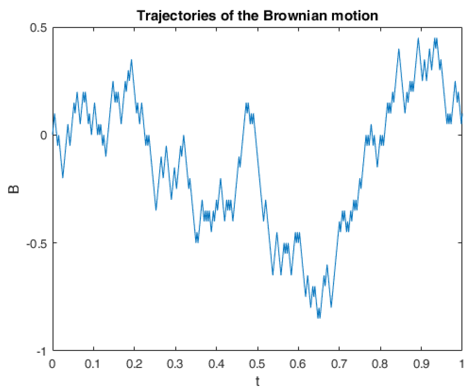
2.1. Random Walk Approximation of the Brownian Motion

We use a random walk to approximate the 1-dimensional standard Brownian motion:
B 0 n = 0 ; B t n : = Δ n j = 1 [ t / Δ n ] ϵ j n , t ( 0 , T ] ; Δ B i n : = B i n B i 1 n = Δ n ϵ i n , i [ 1 , n δ ] ,
where ( ϵ i n ) i = 1 , n is a { 1 , 1 } -value i.i.d. Bernoulli sequence with P ( ϵ i n = 1 ) = P ( ϵ i n = 1 ) = 1 2 . Denote F i n = σ { ϵ 1 n , ϵ i n } , for any i [ 1 , n δ ] . By Donsker’s invariance principle and the Skorokhod representation theorem, there exists a probability space, such that sup 0 t T + δ | B t n B t | 0 , in L 2 ( G T + δ ) , as n .

2.2. Approximation of the Defaultable Model

We consider a defaultable model of a single uniformly distributed random default time τ ( 0 , T ] . We define the discrete default process h i n = h t i n = 1 { τ t i } ( i [ 1 , n ] ). Particularly, when i [ n + 1 , n δ ] , h i n = 1 (since default case already happened). We have the conditional expectations of h i n in G i 1 n :
E h i n = 1 | h i 1 n = 1 = P ( τ t i | τ t i 1 ) = 1 , E h i n = 1 | h i 1 n = 0 = P ( τ t i | τ > t i 1 ) = Δ n T t i 1 , E h i n = 0 | h i 1 n = 0 = P ( τ > t i | τ > t i 1 ) = T t i T t i 1 , i [ 1 , n ] .
We have the following approximation for the discrete martingale M t n directly based on the definition of the martingale M (Assumption 1):
M 0 n = 0 ; M t n : = h [ t / Δ n ] n Δ n j = 1 [ t / Δ n ] ( 1 h j n ) γ j n , t ( 0 , T ] ; Δ M i n : = h i n h i 1 n Δ n ( 1 h i n ) γ i n , i [ 1 , n ] ,
where the discrete intensity process γ i n = γ t i n 0 is an F i n -adapted process. Denote G : = { G i n ; i [ 0 , n δ ] } , G 0 n = { Ω , } , for i [ 1 , n ] , G i n = σ { ϵ 1 n , ϵ i n , h i n } ; for i [ n + 1 , n δ ] , G i n = σ { ϵ 1 n , ϵ i n , h n n } , where h i is independent from ϵ 1 n , … ϵ i n . From the martingale property of M i , we can get
E G i 1 n Δ M i n = E G i 1 n h i n h i 1 n Δ n ( 1 h i n ) γ i n = 0 , i [ 1 , n ] ,
therefore, the discrete intensity process has the following form (by the projection on F i 1 n ):
γ i n = P ( t i 1 < τ t i | F i 1 n ) Δ n P ( τ > t i | F i 1 n ) = 1 T t i , i [ 1 , τ Δ n ] .
Note that γ i n = 0 , when i = 0 and i [ τ Δ n + 1 , n ] . If we set γ ^ t n = γ [ t / Δ n ] n ( t [ 0 , T ] ), then as n , it follows that γ ^ t n converges to γ t .

2.3. Computing the Conditional Expectations

When i [ 1 , n 1 ] , we use the following formula to compute the conditional expectation for the function f : R i + 2 R :
E G i n f ϵ 1 n , , ϵ i + 1 n , h i + 1 n = 1 2 f ϵ 1 n , , ϵ i n , 1 , 1 | ϵ i + 1 n = 1 , h i n = 1 + f ϵ 1 n , , ϵ i n , 1 , 1 | ϵ i + 1 n = 1 , h i n = 1 + Δ n 2 ( T t i ) f ϵ 1 n , , ϵ i n , 1 , 1 | ϵ i + 1 n = 1 , h i n = 0 , h i + 1 n = 1 + f ϵ 1 n , , ϵ i n , 1 , 1 | ϵ i + 1 n = 1 , h i n = 0 , h i + 1 n = 1 + T t i + 1 2 ( T t i ) f ϵ 1 n , , ϵ i n , 1 , 0 | ϵ i + 1 n = 1 , h i n = 0 , h i + 1 n = 0 + f ϵ 1 n , , ϵ i n , 1 , 0 | ϵ i + 1 n = 1 , h i n = 0 , h i + 1 n = 0 .
When i [ n , n δ ] , we have the following conditional expectation for the function f : R i + 2 R :
E G i n f ϵ 1 n , , ϵ i + 1 n , h n n = 1 2 f ϵ 1 n , ϵ i n , 1 , 1 | ϵ i + 1 n = 1 + 1 2 f ϵ 1 n , ϵ i n , 1 , 1 | ϵ i + 1 n = 1 .

2.4. Approximations of the Anticipated Processes and the Generator

Consider the approximation ξ n n of the terminal value ξ , we have the following assumption:
Assumption 6.
( ξ i n ) i [ n , n δ ] is G i n -measurable, Ψ : { 1 , 1 } n R is a real analytic function, such that
ξ i n = Ψ ϵ 1 n , ϵ i n , h i n , i [ n , n δ ] ,
particularly, the terminal value ξ n n = Ψ ϵ 1 n , ϵ n n , h i n is G n n -measurable.
For the approximation f n ( t i , y , y ¯ , z , u ) i [ 0 , n ] of the generator f:
Assumption 7.
for any i [ 0 , n ] , f n ( t i , y , y ¯ , z , u ) is G i n -adapted, and satisfies:
(a) 
there exists a constant C > 0 , such that for all n > 1 + 2 L + 4 L 2 ,
E Δ n i = 0 n 1 | f n ( · , 0 , 0 , 0 , 0 ) | 2 < C .
(b) 
for any i [ 0 , n 1 ] , y, y R , z, z R , u, u R , y ¯ , y ¯ S G 2 ( t , T + δ ; R ) , there exists a constant L 0 , such that
| f n ( t i , y , y ¯ i , z , u ) f n ( t i , y , y ¯ i , z , u ) | L | y y | + E G t | y ¯ i y ¯ i | + | z z | + | u u | 1 { τ > t i } γ i ,
where y ¯ i = E G i n [ y i ¯ ] , i ¯ = i + δ Δ n .
As n , f n ( t Δ n , y , y ¯ , z , u ) converges to f ( t , y , y ¯ , z , u ) in S G 2 ( 0 , T + δ ; R ) .

2.5. Approximation of the Obstacles

( L i n ) i [ 0 , n ] and ( V i n ) i [ 0 , n ] are the discrete versions of L and V, by Assumption 5, we can have the following approximations:
L i n = L 0 + Δ n j = 0 i 1 l j ( 1 ) + j = 0 i 1 l j ( 2 ) Δ B j + 1 n + j = 0 i 1 l j ( 3 ) Δ M j + 1 n ; V i n = V 0 + Δ n j = 0 i 1 v j ( 1 ) + j = 0 i 1 v j ( 2 ) Δ B j + 1 n + j = 0 i 1 v j ( 3 ) Δ M j + 1 n ,
where l j ( k ) = l t j ( k ) , v j ( k ) = v t j ( k ) ( k = 1 , 2 , 3 ). By the Burkholder–Davis–Gundy inequality, it follows
V i n L i n , sup n E sup i ( L i n ) + 2 + sup i ( V i n ) 2 < .
We introduce the discrete version of Assumption 5 (c):
Assumption 8.
There exists a process X i n with the following form:
X i n = X 0 n j = 0 i 1 σ j ( 1 ) Δ B i + 1 n j = 0 i 1 σ j ( 2 ) Δ M i + 1 n + A i + n A i n ,
where A i + n and A i n are G i n -adapted increasing processes, E | A n + n | 2 + | A n n | 2 < , such that
L i n X i n V i n , i [ 0 , n ] .
We introduce two numerical algorithms below, discrete penalization scheme in Section 3 and discrete reflected scheme in Section 4. For each scheme, we study the implicit and explicit versions.

3. Discrete Penalization Scheme

We first use the methodology of penalization for the discrete scheme below. El Karoui et al. (1997a) proved the existence of RBSDE with one obstacle under a smooth square integrability assumption and Lipschitz condition through penalization method. Lepeltier and Martín (2004) used the similar penalization method to prove the existence theorem of RBSDE with two obstacles and Poisson jump. Similarly to Lemma 4.3.1 in Wang (2020), we consider the following special case of the penalized ABSDE for RABSDE (2):
d Y t p = f n t , Y t p , E G t [ Y t + δ p ] , Z t p , U t p d t + d K t + p d K t p Z t p d B t U t p d M t , t [ 0 , T ] , Y t p = ξ t , t [ T , T + δ ] ,
where
K t + p = p t T ( Y s p L s ) d s , K t p = p t T ( Y s p V s ) + d s .
By the existence and uniqueness theorem for ABSDEs with default risk (Theorem 4.3.3 in Wang 2020), there exists the unique solution for this penalized ABSDE (6). We will give the convergence of penalized ABSDE (6) to RABSDE (2) in Theorem 1 below.

3.1. Implicit Discrete Penalization Scheme

We first introduce the implicit discrete penalization scheme. In this scheme, p represents the penalization parameter. In practice, we can choose p which is independent of n and much larger than n, this will be illustrated in the simulation Section 6.
y i p , n = y i + 1 p , n + f n ( t i , y i p , n , y ¯ i p , n , z i p , n , u i p , n ) Δ n + k i + p , n k i p , n z i p , n Δ B i + 1 n u i p , n Δ M i + 1 n , i [ 0 , n 1 ] ; k i + p , n = p Δ n ( y i p , n L i n ) , i [ 0 , n 1 ] ; k i p , n = p Δ n ( y i p , n V i n ) + , i [ 0 , n 1 ] ; y i p , n = ξ i n , i [ n , n δ ] ,
where y ¯ i p , n = E G i n [ y i ¯ p , n ] , i ¯ = i + δ Δ n .
For the theoretical convergence results in Section 5, we first prove the convergence (Theorem 2) of implicit discrete penalization scheme (7) to the penalized ABSDE (6), then combining with Theorem A2, we can get the convergence of the explicit discrete penalization scheme. By Theorem A3 and Theorem 1, we can prove the convergence of the implicit discrete reflected scheme (13).
From Section 2.3, taking conditional expectation in G i n , we can calculate y ¯ i p , n as follows:
E G i n [ y i ¯ p , n ] = 1 2 y i ¯ p , n | ϵ i ¯ n = 1 , h i n = 1 + y i ¯ p , n | ϵ i ¯ n = 1 , h i n = 1 + δ 2 ( T t i ) y i ¯ p , n | ϵ i ¯ n = 1 , h i n = 0 , h i ¯ n = 1 + y i ¯ p , n | ϵ i ¯ n = 1 , h i n = 0 , h i ¯ n = 1 + T t i δ 2 ( T t i ) y i ¯ p , n | ϵ i ¯ n = 1 , h i n = 0 , h i ¯ n = 0 + y i ¯ p , n | ϵ i ¯ n = 1 , h i n = 0 , h i ¯ n = 0 , i ¯ [ i , n 1 ] ; 1 2 ξ i ¯ n | ϵ i ¯ n = 1 + ξ i ¯ n | ϵ i ¯ n = 1 , i ¯ [ n , n δ ] .
Similarly, z i p , n and u i p , n ( i [ 0 , n 1 ] ) are given by
z i p , n = E G i n y i + 1 p , n Δ B i + 1 n E G i n [ ( Δ B i + 1 n ) 2 ] = E G i n y i + 1 p , n Δ n ϵ i + 1 n E G i n [ ( Δ n ϵ i + 1 n ) 2 ] = 1 Δ n E G i n y i + 1 p , n ϵ i + 1 n = y i + 1 p , n | ϵ i + 1 = 1 y i + 1 p , n | ϵ i + 1 = 1 2 Δ n ; u i p , n = E G i n y i + 1 p , n Δ M i + 1 n E G i n [ ( Δ M i + 1 n ) 2 ] = E G i n y i + 1 p , n h i + 1 n h i n Δ n ( 1 h i + 1 n ) γ i + 1 E G i n [ ( h i + 1 n h i n Δ n ( 1 h i + 1 n ) γ i + 1 ) 2 ] = y i + 1 p , n Δ n | h i = 0 , h i + 1 = 1 y i + 1 p , n ( T t i + 1 ) Δ n γ i + 1 | h i = 0 , h i + 1 = 0 Δ n + ( T t i + 1 ) ( Δ n γ i + 1 ) 2 .
Note that u i p , n only exists on [ 0 , τ Δ n 1 ] (i.e., before the default event happens). By taking the conditional expectation of (7) in G i n , it follows:
y i p , n = ( Φ p , n ) 1 E G i n [ y i + 1 n ] , i [ 0 , n 1 ] ; k i + p , n = p Δ n ( y i p , n L i n ) , i [ 0 , n 1 ] ; k i p , n = p Δ n ( y i p , n V i n ) + , i [ 0 , n 1 ] ; y i p , n = ξ i n , i [ n , n δ ] ; z i p , n = 1 Δ n E G i n y i + 1 p , n ϵ i + 1 n , i [ 0 , n 1 ] ; u i p , n = E G i n y i + 1 p , n h i + 1 n h i n Δ n ( 1 h i + 1 n ) γ i + 1 E G i n [ ( h i + 1 n h i n Δ n ( 1 h i + 1 n ) γ i + 1 ) 2 ] , i [ 0 , τ Δ n 1 ] .
where Φ p , n ( y ) = y f n ( t i , y , y ¯ i p , n , z i p , n , u i p , n ) Δ n p Δ n ( y L i n ) + p Δ n ( y V i n ) + . For the continuous time version ( Y t p , n , Z t p , n , U t p , n , K t + p , n , K t p , n ) 0 t T :
Y t p , n : = y [ t / Δ n ] p , n , Z t p , n : = z [ t / Δ n ] p , n , U t p , n : = u [ t / Δ n ] p , n , K t + p , n : = i = 0 [ t / Δ n ] k i + p , n , K t p , n : = i = 0 [ t / Δ n ] k i p , n .

3.2. Explicit Discrete Penalization Scheme

In many cases, the inverse of mapping Φ is not easy to get directly, for example, if f is not a linear function on y. We replace y i p , n in f n by E G i n [ y i + 1 p , n ] in (7), it follows
y ˜ i p , n = y ˜ i + 1 p , n + f n ( t i , E G i n [ y ˜ i + 1 p , n ] , y ˜ ¯ i p , n , z ˜ i p , n , u ˜ i p , n ) Δ n + k ˜ i + p , n k ˜ i p , n z ˜ i p , n Δ B i + 1 n u ˜ i p , n Δ M i + 1 n , i [ 0 , n 1 ] ; k ˜ i + p , n = p Δ n ( y ˜ i p , n L i n ) , i [ 0 , n 1 ] ; k ˜ i p , n = p Δ n ( y ˜ i p , n V i n ) + , i [ 0 , n 1 ] ; y ˜ i p , n = ξ i n , i [ n , n δ ] ,
where y ˜ ¯ i p , n , z ˜ i p , n and u ˜ i p , n can be calculated as (8) and (9). By Section 2.3, we computer E G i n [ y i + 1 p , n ] as follows:
E G i n [ y ˜ i + 1 p , n ] = 1 2 y ˜ i + 1 p , n | ϵ i + 1 n = 1 , h i n = 1 + y ˜ i + 1 p , n | ϵ i + 1 n = 1 , h i n = 1 + Δ n 2 ( T t i ) y ˜ i + 1 p , n | ϵ i + 1 n = 1 , h i n = 0 , h i + 1 n = 1 + y ˜ i + 1 p , n | ϵ i + 1 n = 1 , h i n = 0 , h i + 1 n = 1 + T t i + 1 2 ( T t i ) y ˜ i + 1 p , n | ϵ i + 1 n = 1 , h i n = 0 , h i + 1 n = 0 + y ˜ i + 1 p , n | ϵ i + 1 n = 1 , h i n = 0 , h i + 1 n = 0 .
By taking the conditional expectation of (11) in G i n , we have the following explicit penalization scheme:
y ˜ i p , n = E G i n y ˜ i + 1 p , n + f n ( t i , E G i n [ y ˜ i + 1 p , n ] , y ˜ ¯ i p , n , z ˜ i p , n , u ˜ i p , n ) Δ n + k ˜ i + p , n k ˜ i p , n , i [ 0 , n 1 ] ; k ˜ i + p , n = p Δ n 1 + p Δ n E G i n y ˜ i + 1 p , n + f n ( t i , E G i n [ y ˜ i + 1 p , n ] , y ˜ ¯ i p , n , z ˜ i p , n , u ˜ i p , n ) Δ n L i n , i [ 0 , n 1 ] ; k ˜ i p , n = p Δ n 1 + p Δ n E G i n y ˜ i + 1 p , n + f n ( t i , E G i n [ y ˜ i + 1 p , n ] , y ˜ ¯ i p , n , z ˜ i p , n , u ˜ i p , n ) Δ n V i n + , i [ 0 , n 1 ] ; y ˜ i p , n = ξ i n , i [ n , n δ ] ; z ˜ i p , n = 1 Δ n E G i n y ˜ i + 1 p , n ϵ i + 1 n , i [ 0 , n 1 ] ; u ˜ i p , n = E G i n y ˜ i + 1 p , n h i + 1 n h i n Δ n ( 1 h i + 1 n ) γ i + 1 E G i n [ ( h i + 1 n h i n Δ n ( 1 h i + 1 n ) γ i + 1 ) 2 ] , i [ 0 , τ Δ n 1 ] .
For the continuous time version ( Y ˜ t p , n , Z ˜ t p , n , U ˜ t p , n , K ˜ t + p , n , K ˜ t p , n ) 0 t T :
Y ˜ t p , n : = y ˜ [ t / Δ n ] p , n , Z ˜ t p , n : = z ˜ [ t / Δ n ] p , n , U ˜ t p , n : = u ˜ [ t / Δ n ] p , n , K ˜ t + p , n : = i = 0 [ t / Δ n ] k ˜ i + p , n , K ˜ t p , n : = i = 0 [ t / Δ n ] k ˜ i p , n .
Remark 1.
We give the following explanations of the derivation of k ˜ i + p , n and k ˜ i p , n :
  • If V i n > y ˜ i p , n > L i n , we can get k ˜ i + p , n = k ˜ i p , n = 0 ;
  • If y ˜ i p , n L i n , we can get k ˜ i + p , n = p Δ n 1 + p Δ n ( E G i n y ˜ i + 1 p , n + f n ( t i , E G i n [ y ˜ i + 1 p , n ] , y ˜ ¯ i p , n , z ˜ i p , n , u ˜ i p , n ) Δ n L i n ) , k ˜ i p , n = 0 . From (12), we know that p should be much larger than n to keep y ˜ i p , n above the lower obstacle L i n ;
  • If y ˜ i p , n V i n , we can get k ˜ i p , n = p Δ n 1 + p Δ n ( E G i n y ˜ i + 1 p , n + f n ( t i , E G i n [ y ˜ i + 1 p , n ] , y ˜ ¯ i p , n , z ˜ i p , n , u ˜ i p , n ) Δ n V i n ) + , k ˜ i + p , n = 0 . From (12), we know that p should be much larger than n to keep y ˜ i p , n under the upper obstacle V i n .

4. Discrete Reflected Scheme

We can obtain the solution Y by reflecting between the two obstacles and get the increasing processes K + and K directly.

4.1. Implicit Discrete Reflected Scheme

We have the following implicit discrete reflected scheme,
y i n = y i + 1 n + f n ( t i , y i n , y ¯ i n , z i n , u i n ) Δ n + k i + n k i n z i n Δ B i + 1 n u i n Δ M i + 1 n , i [ 0 , n 1 ] ; V i n y i n L i n , i [ 0 , n 1 ] ; k i + n 0 , k i n 0 , k i + n k i n = 0 , i [ 0 , n 1 ] ; ( y i n L i n ) k i + n = ( y i n V i n ) k i n = 0 , i [ 0 , n 1 ] ; y i n = ξ i n , i [ n , n δ ] .
where y ¯ i n , z i n and u i n can be calculated as (8) and (9). By taking conditional expectation of (13) in G i n , it follows
y i n = E G i n [ y i + 1 n ] + f n ( t i , y i n , y ¯ i n , z i n , u i n ) Δ n + k i + n k i n , i [ 0 , n 1 ] ; V i n y i n L i n , i [ 0 , n 1 ] ; k i + n 0 , k i n 0 , k i + n k i n = 0 , i [ 0 , n 1 ] ; ( y i n L i n ) k i + n = ( y i n V i n ) k i n = 0 , i [ 0 , n 1 ] ; y i n = ξ i n , i [ n , n δ ] ; z i n = 1 Δ n E G i n y i + 1 n ϵ i + 1 n , i [ 0 , n 1 ] ; u i n = E G i n y i + 1 n h i + 1 n h i n Δ n ( 1 h i + 1 n ) γ i + 1 E G i n [ ( h i + 1 n h i n Δ n ( 1 h i + 1 n ) γ i + 1 ) 2 ] , i [ 0 , τ Δ n 1 ] .
If Δ n is small enough, similarly to Section 4.1 in Xu (2011), (14) is equivalent to
y i n = Φ 1 E G i n [ y i + 1 n ] + k i + n k i n , i [ 0 , n 1 ] ; k i + n = E G i n [ y i + 1 n ] + f n ( t i , L i n , L ¯ i n , z i n , u i n ) Δ n L i n , i [ 0 , n 1 ] ; k i n = E G i n [ y i + 1 n ] + f n ( t i , V i n , V ¯ i n , z i n , u i n ) Δ n V i n + , i [ 0 , n 1 ] ; y i n = ξ i n , i [ n , n δ ] ; z i n = 1 Δ n E G i n y i + 1 n ϵ i + 1 n , i [ 0 , n 1 ] ; u i n = E G i n y i + 1 n h i + 1 n h i n Δ n ( 1 h i + 1 n ) γ i + 1 E G i n [ ( h i + 1 n h i n Δ n ( 1 h i + 1 n ) γ i + 1 ) 2 ] , i [ 0 , τ Δ n 1 ] .
here Φ ( y ) = y f n ( t i , y , y ¯ i n , z i n , u i n ) Δ n . For the continuous time version ( Y t n , Z t n , U t n , K t + n , K t n ) 0 t T :
Y t n : = y [ t / Δ n ] n , Z t n : = z [ t / Δ n ] n , U t n : = u [ t / Δ n ] n , K t + n : = i = 0 [ t / Δ n ] k i + n , K t n : = i = 0 [ t / Δ n ] k i n .

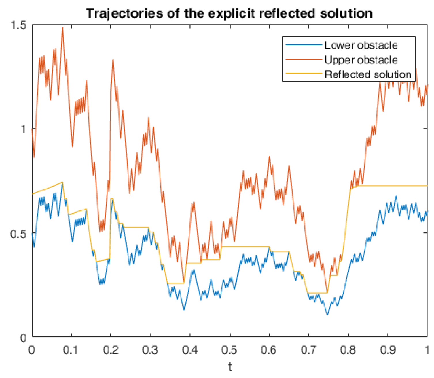
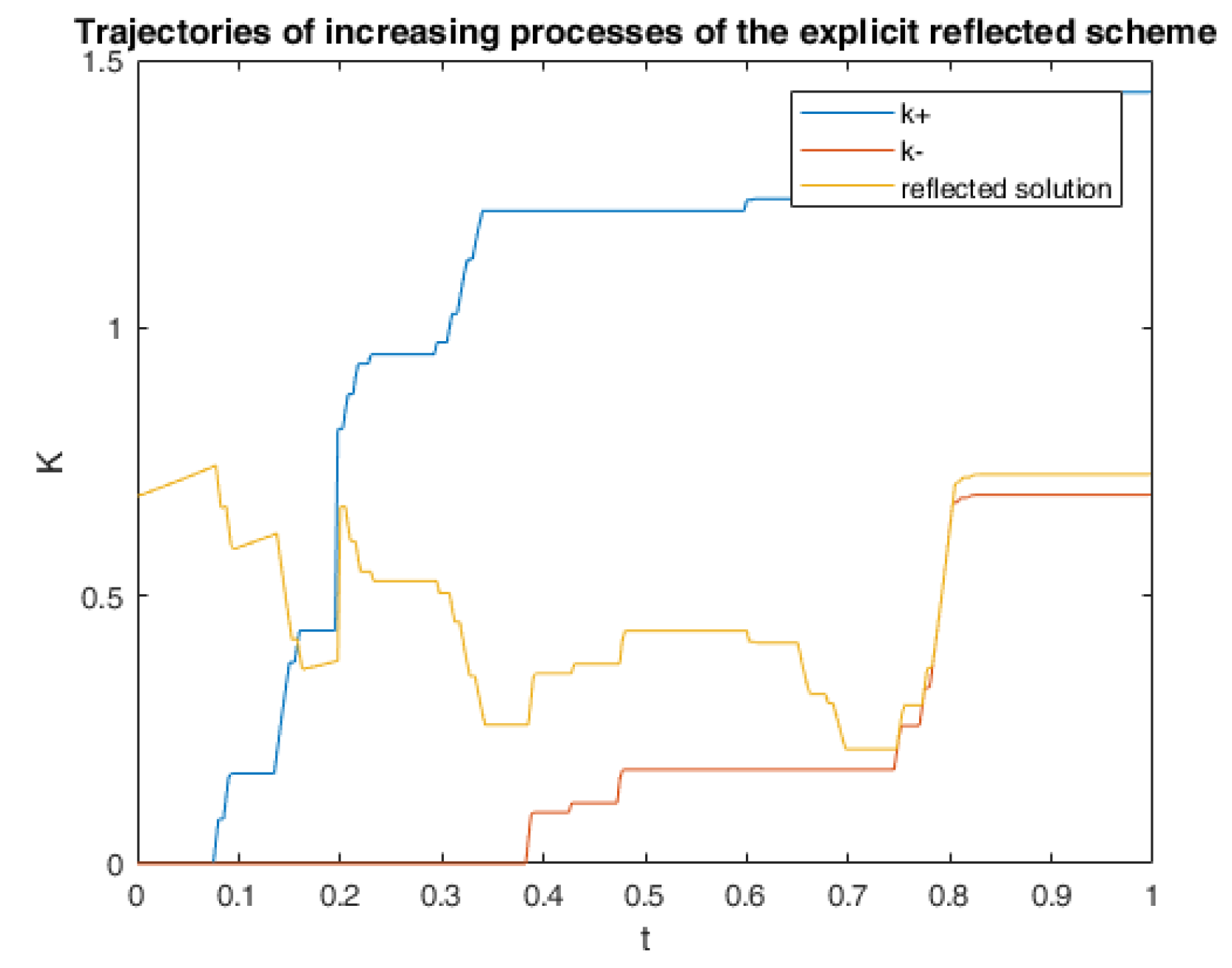
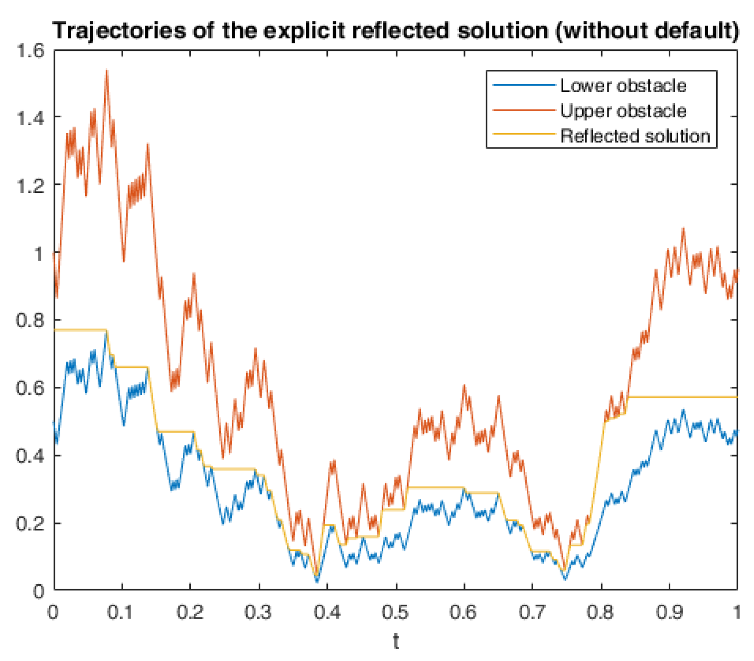
4.2. Explicit Discrete Reflected Scheme

We introduce the following explicit discrete reflected scheme by replacing y i n in the generator f n by E [ y i + 1 n | G i n ] in (13).
y ˜ i n = y ˜ i + 1 n + f n ( t i , E G i n [ y ˜ i + 1 n ] , y ˜ ¯ i n , z ˜ i n , u ˜ i n ) Δ n + k ˜ i + n k ˜ i n z ˜ i n Δ B i + 1 n u ˜ i n Δ M i + 1 n , i [ 0 , n 1 ] ; V i n y ˜ i n L i n , i [ 0 , n 1 ] ; k ˜ i + n 0 , k ˜ i n 0 , k ˜ i + n k ˜ i n = 0 , i [ 0 , n 1 ] ; ( y ˜ i n L i n ) k ˜ i + n = ( y ˜ i n V i n ) k ˜ i n = 0 , i [ 0 , n 1 ] ; y ˜ i n = ξ i n , i [ n , n δ ] .
where y ˜ ¯ i n , z ˜ i n and u ˜ i n can be calculated as (8) and (9). By taking conditional expectation of (16) in G i n :
y ˜ i n = E G i n [ y ˜ i + 1 n ] + f n ( t i , E G i n [ y ˜ i + 1 n ] , y ˜ ¯ i n , z ˜ i n , u ˜ i n ) Δ n + k ˜ i + n k ˜ i n , i [ 0 , n 1 ] ; V i n y ˜ i n L i n , i [ 0 , n 1 ] ; k ˜ i + n 0 , k ˜ i n 0 , k ˜ i + n k i n = 0 , i [ 0 , n 1 ] ; ( y ˜ i n L i n ) k ˜ i + n = ( y ˜ i n V i n ) k ˜ i n = 0 , i [ 0 , n 1 ] ; y ˜ i n = ξ i n , i [ n , n δ ] ; z ˜ i n = 1 Δ n E G i n y ˜ i + 1 n ϵ i + 1 n , i [ 0 , n 1 ] ; u ˜ i p , n = E G i n y ˜ i + 1 n h i + 1 n h i n Δ n ( 1 h i + 1 n ) γ i + 1 E G i n [ ( h i + 1 n h i n Δ n ( 1 h i + 1 n ) γ i + 1 ) 2 ] , i [ 0 , τ Δ n 1 ] .
Similarly to the implicit reflected case, we can obtain
y ˜ i n = E G i n [ y ˜ i + 1 n ] + f n ( t i , E G i n [ y ˜ i + 1 n ] , y ˜ ¯ i n , z ˜ i n , u ˜ i n ) Δ n + k ˜ i + n k ˜ i n , i [ 0 , n 1 ] ; k ˜ i + n = E G i n [ y ˜ i + 1 n ] + f n ( t i , E G i n [ y ˜ i + 1 n ] , y ˜ ¯ i n , z ˜ i n , u ˜ i n ) Δ n L i n , i [ 0 , n 1 ] ; k ˜ i n = E G i n [ y ˜ i + 1 n ] + f n ( t i , E G i n [ y ˜ i + 1 n ] , y ˜ ¯ i n , z ˜ i n , u ˜ i n ) Δ n V i n + , i [ 0 , n 1 ] ; y ˜ i n = ξ i n , i [ n , n δ ] ; z ˜ i n = 1 Δ n E G i n y ˜ i + 1 n ϵ i + 1 n , i [ 0 , n 1 ] ; u ˜ i p , n = E G i n y ˜ i + 1 n h i + 1 n h i n Δ n ( 1 h i + 1 n ) γ i + 1 E G i n [ ( h i + 1 n h i n Δ n ( 1 h i + 1 n ) γ i + 1 ) 2 ] , i [ 0 , τ Δ n 1 ] .
For the continuous time version ( Y ˜ t n , Z ˜ t n , U ˜ t n , K ˜ t + n , K ˜ t n ) 0 t T :
Y ˜ t n : = y ˜ [ t / Δ n ] n , Z ˜ t n : = z ˜ [ t / Δ n ] n , U ˜ t n : = u ˜ [ t / Δ n ] n , K ˜ t + n : = i = 0 [ t / Δ n ] k ˜ i + n , K ˜ t n : = i = 0 [ t / Δ n ] k ˜ i n .

5. Convergence Results

We first state the convergence result from the Penalized ABSDE (19) to RABSDE (2) in Theorem 1, which is the basis of the following convergence results of the discrete schemes we have studied above. We prove the convergence (Theorem 2) from the implicit discrete penalization scheme (7) to the penalized ABSDE (6) with the help of Lemma 1. Combining with Theorem A2, we can get the convergence (Theorem 3) of the explicit discrete penalization scheme (11). By Theorem A3, Lemma 1 and Theorem 1, we can prove the convergence of the implicit discrete reflected scheme (13). By Theorem A3, Theorem A4 and Lemma A4, the convergence (Theorem 5) of the explicit penalization discrete scheme (16) then follows. The proofs of Theorem 1, Lemma 1, Theorem 2 and Theorem 4 can be seen in Appendix A.

5.1. Convergence of the Penalized ABSDE to RABSDE (2)

Theorem 1.
Suppose that the anticipated process ξ, the generator f satisfy Assumption 3 and Assumption 4, f ( t , y , y ¯ r , z , u ) is increasing in y ¯ , the obstacles L and V satisfy Assumption 5. We can consider the following special case of the penalized ABSDE for RABSDE (2):
d Y t p = f n t , Y t p , E G t [ Y t + δ p ] , Z t p , U t p d t + d K t + p d K t p Z t p d B t U t p d M t , t [ 0 , T ] ; K t + p = 0 t p ( Y s p L s ) d s , t [ 0 , T ] ; K t p = 0 t p ( Y s p V s ) + d s , t [ 0 , T ] ; Y t p = ξ t , t [ T , T + δ ] .
Then we have the limiting process ( Y , Z , U , K + , K ) of ( Y p , Z p , U p , K + p , K p ) , i.e., as p , Y t p Y t in S G 2 ( 0 , T + δ ; R ) , Z t p Z t weakly in L G 2 ( 0 , T ; R ) , U t p U t weakly in L G 2 , τ ( 0 , T ; R ) , K t + p ( K t p ) K t + ( K t ) weakly in A G 2 ( 0 , T ; R ) . Moreover, there exists a constant C ξ , f , L , V depending on ξ, f ( t , 0 , 0 , 0 , 0 ) , L and V, such that
E [ sup 0 t T | Y t p Y t | 2 + 0 T | Z t p Z t | 2 d t + 0 T | U t p U t | 2 1 { τ > t } γ t d t + sup 0 t T | ( K t + p K t + ) ( K t p K t ) | 2 ] 1 p C ξ , f , L , V .

5.2. Convergence of the Implicit Discrete Penalization Scheme

We first introduce the following lemma to prove the convergence result of the penalized ABSDE (19) to the implicit penalization scheme.
Lemma 1.
Under Assumption 6 and Assumption 7, ( Y t p , n , Z t p , n , U t p , n ) converges to ( Y t p , Z t p , U t p ) in the following sense:
lim n E sup 0 t T | Y t p , n Y t p | 2 + 0 T | Z t p , n Z t p | 2 d t + 0 T | U t p , n U t p | 2 1 { τ > t } γ t d t = 0 ,
for any t [ 0 , T ] , as n , K t + p , n K t p , n K t + p K t p in L G 2 ( 0 , T ; R ) .
Theorem 2.
(Convergence of the implicit discrete penalization scheme) Under Assumption 3 and Assumption 7, ( Y t p , n , Z t p , n , U t p , n ) converges to ( Y t , Z t , U t ) in the following sense:
lim p lim n E sup 0 t T | Y t p , n Y t | 2 + 0 T | Z t p , n Z t | 2 d t + 0 T | U t p , n U t | 2 1 { τ > t } γ t d t = 0 ,
for any t [ 0 , T ] , as p , n , K t + p , n K t p , n K t + K t in L G 2 ( 0 , T ; R ) .

5.3. Convergence of the Explicit Discrete Penalization Scheme

By Theorem 2 and Theorem A2, we can obtain the following convergence result of the explicit penalization discrete scheme.
Theorem 3.
(Convergence of the explicit discrete penalization scheme) Under Assumption 3 and Assumption 7, ( Y ˜ t p , n , Z ˜ t p , n , U ˜ t p , n ) converges to ( Y t , Z t , U t ) in the following sense:
lim n E sup 0 t T | Y ˜ t p , n Y t | 2 + 0 T | Z ˜ t p , n Z t | 2 d t + 0 T | U ˜ t p , n U t | 2 1 { τ > t } γ t d t = 0 ,
for any t [ 0 , T ] , as n , K ˜ t + p , n K ˜ t p , n K t + K t in L G 2 ( 0 , T ; R ) .

5.4. Convergence of the Implicit Discrete Reflected Scheme

Theorem 4.
(Convergence of the implicit discrete reflected scheme) Under Assumption 7 and Assumption 3, ( Y t n , Z t n , U t n ) converges to ( Y t , Z t , U t ) in the following sense:
lim n E sup 0 t T | Y t n Y t | 2 + 0 T | Z t n Z t | 2 d t + 0 T | U t n U t | 2 1 { τ > t } γ t d t = 0 ,
and for any t [ 0 , T ] , as n , K t + n K t n K t + K t in L G 2 ( 0 , T ; R ) .

5.5. Convergence of the Explicit Discrete Reflected Scheme

By Theorem A3, Theorem A4 and Lemma A4, we can get the convergence result of the explicit penalization discrete scheme.
Theorem 5.
(Convergence of the explicit discrete reflected scheme) Under Assumption 3 and Assumption 7, ( Y ˜ t n , Z ˜ t n , U ˜ t n ) converges to ( Y t , Z t , U t ) in the following sense:
lim n E sup 0 t T | Y ˜ t n Y t | 2 + 0 T | Z ˜ t n Z t | 2 d t + 0 T | U ˜ t n U t | 2 1 { τ > t } γ t d t = 0 ,
for any t [ 0 , T ] , as n , K ˜ t + n K ˜ t n K t + K t in L G 2 ( 0 , T ; R ) .

6. Numerical Calculations and Simulations

6.1. One Example of RABSDE with Two Obstacles and Default Risk

For the convenience of computation, we consider the case when the terminal time T = 1 , the calculation begins from y n n = ξ n , and proceeds backward to solve ( y i n , z i n , u i n , k i + n , k i n ) for i = n 1 , n 2 , , 1 , 0 . We use Matlab for the simulation. We consider a simple situation: the terminal value ξ T = Φ ( B T , M T ) and anticipated process ξ t = Φ ( B t ) ( t ( T , T + δ ] ); the obstacles L t = Ψ 1 ( t , B t , M t ) and V t = Ψ 2 ( t , B t , M t ) , where Φ , Ψ 2 and Ψ 3 are real analytic functions defined on R , [ 0 , T ] × R and [ 0 , T ] × R respectively. We take the following example ( n = 200 , anticipated time δ = 0.3 ):
f ( t , y , y ¯ , z , u ) = y 2 + y ¯ 2 + z + u , t [ 0 , T ] ; Φ ( B t ) = | B t | + M T , t [ T , T + δ ] ; Ψ 1 ( t , B t , M t ) = | B t | + M t + T t , t [ 0 , T ] ; Ψ 2 ( t , B t , M t ) = | B t | + M t + 2 T t , t [ 0 , T ] ;
This example satisfies the Assumption 3, Assumption 4 and Assumption 5 in the theoretical Section 1.3. We choose the default time τ as a uniformly distributed random variable.
As the inverse for both implicit schemes in (10) and (15) is not easy to get directly, we only use explicit schemes below. We are going to illustrate the behaviors of the explicit reflected scheme by looking at the pathwise behavior for n = 400 . Further, we will compare the explicit reflected scheme with the explicit penalization scheme for different values of the penalization parameter.
Figure 1 represents one path of the Brownian motion, Figure 2 and Figure 3 represent one path of the Brownian motion and one path of the default martingale when the default time τ = 0.7 and 0.2 respectively.
Figure 4 and Figure 5 represent the paths of the solution y ˜ n , increasing processes K ˜ + n and K ˜ n in the explicit reflected scheme where the random default time τ = 0.7 . We can see that for all i, y ˜ i n stays between the lower obstacle L i n and the upper obstacle V i n , the increasing process K ˜ i + n (resp. K ˜ i n ) pushes y ˜ i n upward (resp. downward), and they can not increase at the same time. In this example for n = 400 , default time τ = 0.7 , we can get the reflected solution y ˜ 0 n = 1.2563 from the explicit reflected scheme.
Figure 4 and Figure 6 illustrate the influence of the jump on the solution y ˜ n at the different random default times, the reflected solution y ˜ n moves downwards after the default time (which can not be shown in Figure 7). From the approximation of the default martingale (5), M n is larger with a larger default time.
Table 1 and contains the comparison between the explicit reflected scheme and the explicit penalization scheme by the values of y ˜ 0 n and y ˜ 0 p , n with respect to the parameters n and p. As n increases, the reflected solution y ˜ 0 n increases because of the choice of the coefficient. For fixed n, as the penalization parameter p increases, the penalization solution y ˜ 0 p , n converges increasingly to the reflected solution y ˜ 0 n , which is obvious from the comparison theorem of BSDE with default risk. If p and n have a smaller difference (when n = 10 3 , p = 10 3 ), the penalization solution y ˜ 0 p , n is far from the reflected solution y ˜ 0 n . Hence, the penalization parameter p should be chosen as large as possible. Table 2 illustrates the comparison between the reflected solution y ˜ 0 n and y ˜ 0 n . Figure 7 represents the situation without the default risk, the reflected solution y ˜ 0 n has a larger value than in the situation when the default case happens (Figure 4).

6.2. Application in American Game Options in a Defaultable Setting

6.2.1. Model Description

Hamadene (2006) studied the relation between American game options and RBSDE with two obstacles driven by Brownian motion. In our paper, we consider the case with default risk. An American game option contract with maturity T involves a broker c 1 and a trader c 2 :
  • The broker c 1 has the right to cancel the contract at any time before the maturity T, while the trader c 2 has the right to early exercise the option;
  • the trader c 2 pays an initial amount (the price of this option) which ensures an income L τ 1 from the broker c 1 , where τ 1 [ 0 , T ] is an G -stopping time;
  • the broker has the right to cancel the contract before T and needs to pay V τ 2 to c 2 . Here, the payment amount of the broker c 1 should be greater than his payment to the trader c 2 (if trader decides for early exercise), i.e., V τ 2 L τ 2 , V τ 2 L τ 2 is the premium that the broker c 1 pays for his decision of early cancellation. τ 2 [ 0 , T ] is an G -stopping time;
  • if c 1 and c 2 both decide to stop the contract at the same time τ , then the trader c 2 gets an income equal to Q τ 1 { τ < T } + ξ 1 { τ = T } .

6.2.2. The Hedge for the Broker

Consider a financial market M , we have a riskless asset C t R with risk-free rate r:
d C t = r C t d t , t ( 0 , T ] , C 0 = c 0 , t = 0 ;
one risky asset S t R :
d S t = S t μ d t + σ d B t + χ d M t , t ( 0 , T ] , S 0 = s 0 , t = 0 ,
where B t is a 1-dimensional Brownian Motion, μ is the expected return, σ is the volatility, χ is the parameter related to the default risk.
Consider a self-financing portfolio π R d with strategy π = β s ( 1 ) , β s ( 2 ) s [ t , T ] trading on C and S respectively on the time interval [ t , T ] . A π , α is the wealth process with the value α A at time t, here is a non-negative F t -measurable random variable.
A s π , α = β s ( 1 ) C s + β s ( 2 ) S s , s [ t , T ] ; A s π , α = α A + t s β u ( 1 ) d C u + t s β u ( 2 ) d S u , s [ t , T ] ; t T | β u ( 1 ) | + ( β u ( 2 ) S u ) 2 d u < ;
Let L π , α be a positive local martingale with the following form:
d L t π , α = L t π , α σ 1 ( μ r ) d B t , t ( 0 , T ] , L 0 π , α = 1 , t = 0 ,
By Girsanov’s theorem, let P π , α be the equivalent measure of P :
P π , α P | G T = L T π , α = exp σ 1 ( μ r ) B T 1 2 σ 1 ( μ r ) 2 T ,
here let E π , α be the expectation, B π , α and M π , α be the Brownian motion and the default martingale under the measure P π , α :
B t π , α : = B t + σ 1 ( μ r ) t ; M t π , α : = M t .
Hence, the risky asset S t defined in (26) can be converted into the following form under measure P π , α :
d S t = S t r d t + σ d B t π , α + χ d M t π , α , t ( 0 , T ] , S 0 = s 0 , t = 0 .
Denote by ( π , θ ) a hedge for the broker against the American game option after t, where π is defined in (27), θ [ t , T ] is a stopping time, satisfying
A s π , α R ( s , θ ) : = V θ 1 { θ < s } + L s 1 { s < θ } + Q s 1 { θ = s < T } + ξ 1 { θ = s = T } , s [ t , T ] , P a . s .
here R ( s , θ ) is the amount that the broker c 1 has to pay if the option is exercised by c 2 at s or canceled at time θ . Similarly to El Karoui et al. (1997b) and Karatzas and Shreve (1998), we define the value of the option at time t by J t , where ( J t ) 0 t T is an rcll (right continuous with left limits) process, for any t [ 0 , T ] ,
J t : = e s s inf { α A 0 ; G t - measurable such that there exists a hedge ( π , θ ) after t , where π is a self - financing portfolio after t whose value at t is α A . }
Consider the following RBSDE with two obstacles and default risk, for any t [ 0 , T ] , there exist a stopping time θ t , a process Z s π , α t s T and increasing processes K s π , α + t s T and K s π , α t s T , such that
Y t π , α = Y θ t π , α + K θ t π , α , + K s π , α , + K θ t π , α K s π , α s θ t Z u π , α d B u π , α s θ t U u π , α d M u π , α , s [ t , θ t ] ; Y T π , α = e r T ξ ; e r s L s Y s π , α e r s V s , s [ t , T ] ; t θ t ( Y u π , α e r u L u ) d K u π , α + = t θ t ( e r u V u Y u π , α ) d K u π , α = 0 ;
For any s [ t , T ] , e r t Y t π , α is a hedge for the broker c 1 against the game option, i.e., J t = e r t Y t π , α (see Theorem A5 in the Appendix). Similarly to Proposition 4.3 in Hamadene (2006), we set
θ t : = inf s t ; Y t π , α = e r s V s T = inf s t ; K s π , α > 0 ; v t : = inf s t ; Y t π , α = e r s L s T = inf s t ; K s π , α + > 0 ,
therefore, we can get
R ^ t ( v , θ t ) Y t π , α = R ^ t ( v t , θ t ) R ^ t ( v t , θ ) ,
where
R ^ t ( v , θ ) : = E π , α e r θ V θ 1 { θ < v } + e r v L v 1 { v < θ } + e r θ Q θ 1 { θ = v < T } + e r T ξ 1 { θ = v = T } | G t , P a . s .

6.2.3. Numerical Simulation

We use the same calculation method as in Section 6.1, starting from Y n π , α = ξ , and proceeding backward to solve ( Y i π , α , Z i π , α , U i π , α , K i π , α + , K i π , α ) for i = n 1 , , 1 , 0 with step size Δ n . The forward SDEs (25) and (26) can be numerically approximated by the Euler scheme on the time grid ( t i ) i = 0 , 1 , n :
C i + 1 = C i + r C i Δ n ; S i + 1 = S i + S i μ Δ n + σ Δ B i n + χ Δ M i n .
In this case, we consider parameters as below:
s 0 = 1.5 , T = 1 , r = 1.1 , μ = 1.5 , σ = 0.5 , χ = 0.2 , L t = S t 1 + , V t = 2 S t 1 + , ξ = 1.2 S T 1 + ,
In the case n = 400 , Figure 8 represents one path of the Brownian motion, Figure 9 and Figure 10 represent the paths of the solution Y π , α , increasing processes K π , α and K π , α in the explicit reflected scheme where the random default time τ = 0.2 . We can see that Y t π , α stays between the lower obstacle e r t L t and the upper obstacle e r t V t . In this example for n = 400 , default time τ = 0.2 , we can get the solution Y 0 π , α = 0.6857 from the explicit reflected scheme, i.e., the hedge for the broker c 1 against the game option at t = 0 in the defaultable model. In the case without the default risk, Y 0 π , α = 0.7704 , which means the occurrence of the default event could reduce the value of Y π , α . Figure 11 represents the situation without the default risk, the solution Y π , α has a larger value than in the situation when the default case happens (Figure 9).

Author Contributions

Both two authors have contributed to the final version of the manuscript, and have read and agreed to the published version of the manuscript. This paper is one part of Jingnan Wang’s doctoral dissertation (Wang 2020), Ralf Korn is Jingnan Wang’s PhD supervisor. For this manuscript, Jingnan Wang developed the theoretical formalism and completed the numerical simulations through Matlab. Ralf Korn supervised the work, discussed several versions of the research with Jingnan Wang and assisted in the transformation of the research to this article format. All authors have read and agreed to the published version of the manuscript.

Funding

Jingnan Wang’s work has been carried out as a member of the DFG Research Training Group 1932 “Stochastic Models for Innovations in the Engineering Sciences. The funding by DFG is gratefully aknowledged.

Acknowledgments

We acknowledge the PhD seminar held in our department every week to exchange research progress and bring new insights.

Conflicts of Interest

The authors declare no conflict of interest.

Appendix A

Lemma A1.
(Discrete Gronwall’s Inequality) (Lemma 2.2 in Mémin et al. 2008)
Suppose that a, b and c are positive constants, b Δ < 1 , ( β i ) i N is a sequence with positive values, such that
β i + c a + b Δ j = 1 i β j , i N ,
then it follows
sup i n β i + c a F Δ ( b ) ,
where F Δ ( b ) is a convergent series with the following form:
F Δ ( b ) = 1 + n = 1 b n n ( 1 + Δ ) 1 + ( n 1 ) Δ .
Theorem A1.
(Itô’s formula for rcll semi-martingale) (Protter 2005)
Let X : = ( X t ) 0 t T be a rcll semi-martingale, g is a real value function in C 2 , therefore, g ( X ) is also a semi-martingale, such that
g ( X t ) = g ( X 0 ) + 0 t g ( X s ) d X s + 1 2 0 t g ( X s ) d [ X ] s c + 0 < s t g ( X s ) g ( X s ) g ( X s ) Δ X s .
where [ X ] is the second variation of X, [ X ] c is the continuous part of [ X ] , Δ X s = Δ X s Δ X s .
We give the proofs of Theorem 1, Lemma 1, Theorem 2 and Theorem 4 can be seen in Section 5.
Proof of Theorem 1. 
Firstly, we introduce the following ABSDE:
d Y t p , q = f t , Y t p , q , E G t [ Y t + δ p , q ] , Z t p , q , U t p , q d t + q ( Y t p , q L t ) d t p ( Y t p , q V t ) + d t Z t p , q d B t U t p , q d M t , t [ 0 , T ] .
By the existence and uniqueness theorem for ABSDEs with default risk (Theorem 4.3.3 in Wang 2020), there exists the unique solution for ABSDE (A1). It follows that as q , Y t p , q Y ̲ t p in S G 2 ( 0 , T + δ ; R ) , Z t p , q Z ̲ t p in L G 2 ( 0 , T ; R ) , U t p , q U ̲ t p in L G 2 , τ ( 0 , T ; R ) , 0 t q ( Y s p , q L s ) d s K ̲ t p in A G 2 ( 0 , T ; R ) . ( Y ̲ p , Z ̲ p , U ̲ p , K ̲ p ) is a solution of the following RABSDE with one obstacle L:
d Y ̲ t p = f t , Y ̲ t p , E G t [ Y ̲ t + δ p ] , Z ̲ t p , U ̲ t p d t + d K ̲ t p p ( Y ̲ t p V t ) + d t Z ̲ t p d B t U ̲ t p d M t , t [ 0 , T ] .
Let p , it follows that Y ̲ t p Y t in S G 2 ( 0 , T + δ ; R ) , Z ̲ t p Z t in L G 2 ( 0 , T ; R ) , U ̲ t p U t in L G 2 , τ ( 0 , T ; R ) . By the comparison theorem for ABSDEs with default risk (Theorem 2.3.1 in Wang 2020), we know that K ̲ t p is increasing, then K ̲ T p K T + p and K ̲ T p + 1 K ̲ T p sup 0 t T [ K ̲ t p + 1 K ̲ t p ] 0 , therefore, K ̲ t p K t + p in A G 2 ( 0 , T ; R ) . Hence, there exists a constant C 1 depending on ξ , f ( t , 0 , 0 , 0 , 0 ) , δ , L and V, such that
E sup 0 t T Y ̲ t p Y t 2 + 0 T Z ̲ t p Z t 2 d t + 0 T U ̲ t p U t 2 1 { τ > t } γ t d t C 1 p .
Similarly, let p in (A1), it follows that Y t p , q Y ¯ t q in S G 2 ( 0 , T + δ ; R ) , Z t p , q Z ¯ t p in L G 2 ( 0 , T ; R ) , U t p , q U ¯ t p in L G 2 , τ ( 0 , T ; R ) , 0 t p ( Y ̲ s p V s ) + d s K ¯ t q in A G 2 ( 0 , T ; R ) . ( Y ¯ q , Z ¯ q , U ¯ q , K ¯ q ) is a solution of the following RABSDE with one obstacle V:
d Y ¯ t q = f t , Y ¯ t q , E G t [ Y ¯ t + δ q ] , Z ¯ t q , U ¯ t q d t + q ( Y ¯ t q L t ) d t d K ¯ t q Z ¯ t q d B t U ¯ t q d M t , t [ 0 , T ] .
Letting q , it follows that Y ¯ t q Y t in S G 2 ( 0 , T + δ ; R ) , Z ¯ t q Z t in L G 2 ( 0 , T ; R ) , U ¯ t q U t in L G 2 , τ ( 0 , T ; R ) , K ¯ t p K t p in A G 2 ( 0 , T ; R ) . Moreover, there exists a constant C 2 depending on ξ , f ( t , 0 , 0 , 0 , 0 ) , δ , L and V, such that
E sup 0 t T Y ¯ t q Y t 2 + 0 T Z ¯ t q Z t 2 d t + 0 T U ¯ t q U t 2 1 { τ > t } γ t d t C 2 q .
By the comparison theorem for ABSDEs with default risk, it follows that Y ̲ t p Y t p Y ¯ t p , for any t [ 0 , T ] . Therefore,
E sup 0 t T Y t p Y t 2 C 3 p ,
where C 3 0 is a constant. Applying Itô formula for rcll semi-martingale (Theorem A1), we can obtain
E 0 T | Z t p Z t | 2 d t + 0 T | U t p U t | 2 1 { τ > t } γ t d t C 4 p ,
where C 4 0 is a constant. Since
K t + p K t p = Y 0 p Y t p 0 t f s , Y s p , E G s [ Y s + δ p ] , Z s p , U s p d s 0 t Z s p d B s 0 t U s p d M s ; K t + K t = Y 0 Y t 0 t f s , Y s , E G s [ Y s + δ ] , Z s , U s d s 0 t Z s d B s 0 t U s d M s .
By the convergence of Y p , Z p , U p and the Lipschitz condition of f, it follows
E sup 0 t T | ( K t + p K t + ) ( K t p K t ) | 2 λ E sup 0 t T Y t p Y t 2 + 0 T | Z t p Z t | 2 d t + 0 T | U t p U t | 2 1 { τ > t } γ t d t C 5 p ,
where λ , C 5 0 are constants. Since E [ | K T + p | 2 + | K T p | 2 ] < , there exist processes K ^ + and K ^ in A G 2 ( 0 , T ; R ) are the weak limits of K + p and K p respectively. Since for any t [ 0 , T ] , Y ̲ t p Y t p Y ¯ t p , we can get
d K t + p = p ( Y t p L t ) d t p ( Y ¯ t p L t ) d t = d K ¯ t + p ; d K t p = p ( Y t p V t ) + d t p ( Y ̲ t p V t ) + d t = d K ̲ t p .
Therefore, d K ^ t + d K t + , d K ^ t d K t , it follows that d K ^ t + d K ^ t d K t + d K t . On the other hand, the limit of Y p is Y, so d K ^ t + d K ^ t = d K t + d K t , it follows that d K ^ t + = d K t + , d K ^ t = d K t , then K ^ t + = K t + , K ^ t = K t . □
Proof of Lemma 1.
Step 1. Firstly, we consider the continuous and discrete time equations by Picard’s method.
In the continuous case, we set Y p , , 0 = Z p , , 0 = U p , , 0 = 0 , ( Y t p , , m + 1 , Z t p , , m + 1 , U t p , , m + 1 ) is the solution of the following BSDE:
Y t p , , m + 1 = ξ T + t T f n s , Y s p , , m , E G s [ Y s + δ p , , m ] , Z s p , , m , U s p , , m d s + t T q ( Y s p , , m L s ) d s t T p ( Y s p , , m V s ) + d s t T Z s p , , m + 1 d B s t T U s p , , m + 1 d M s , t [ 0 , T ] ; Y t p , , m + 1 = ξ t , t ( T , T + δ ] ,
where ( Y t p , , m , Z t p , , m , U t p , , m ) is the Picard approximation of ( Y t p , Z t p , U t p ) .
In the discrete case, we set y i p , n , 0 = z i p , n , 0 = u i p , n , 0 = 0 (for any i = 0 , 2 , n ), ( y i p , n , m + 1 , z i p , n , m + 1 , u i p , n , m + 1 ) is the solution of the following BSDE:
y i p , n , m + 1 = y i + 1 p , n , m + 1 + f n ( t i , y i p , n , m , y ¯ i p , n , m , z i p , n , m , u i p , n , m ) Δ n z i p , n , m + 1 Δ B i + 1 n u i p , n , m + 1 Δ M i + 1 n + p Δ n ( y i p , n L i n ) p Δ n ( y i p , n V i n ) + , i [ 0 , n 1 ] ; y i p , n , m + 1 = ξ i n , i [ n , n δ ] .
here ( Y t p , n , m , Z t p , n , m , U t p , n , m ) is the continuous time version of the discrete Picard approximation of ( y i p , n , m , z i p , n , m , u i p , n , m ) .
Step 2. Then, we consider the following decomposition:
Y p , n Y p = Y p , n Y p , n , m + Y p , n , m Y p , , m + Y p , , m Y p .
From Proposition 1 and Proposition 3 in Lejay et al. (2014) and the definition of L i n and V i n , it follows (20). □
Proof of Theorem 2.
By Lemma 1 and Theorem 1, as p , n , it follows
E sup 0 t T | Y t p , n Y t | 2 + 0 T | Z t p , n Z t | 2 d t + 0 T | U t p , n U t | 2 1 { τ > t } γ t d t 2 E sup 0 t T | Y t p , n Y t p | 2 + 0 T | Z t p , n Z t p | 2 d t + 0 T | U t p , n U t p | 2 1 { τ > t } γ t d t + 2 E sup 0 t T | Y t p Y t | 2 + 0 T | Z t p Z t | 2 d t + 0 T | U t p U t | 2 1 { τ > t } γ t d t 0 .
For the increasing processes K + p , n and K p , n , by Theorem 1, we can obtain
E K t + p , n K t p , n K t + K t 2 2 E K t + p , n K t p , n K t + p K t p 2 + C p ,
where C 0 is a constant depending on ξ , f ( t , 0 , 0 , 0 , 0 ) , δ , L and V. For each fixed p,
K t + p , n K t p , n = Y 0 p , n Y t p , n 0 t f n s , Y s p , n , E G s [ Y s + δ p , n ] , Z s p , n , U s p , n d s 0 t Z s p , n d B s n 0 t U s p , n d M s n ; K t + p K t p = Y 0 p Y t p 0 t f s , Y s p , E G s [ Y s + δ p ] , Z s p , U s p d s 0 t Z s p d B s 0 t U s p d M s .
From Corollary 14 in Briand et al. (2002), we know that as n , 0 · Z s p , n d B s n 0 · Z s p d B s in S G 2 ( 0 , T ; R ) , 0 · U s p , n d M s n 0 · U s p d M s in S G 2 ( 0 , T ; R ) . By the Lipschitz condition of f and the convergence of Y p , n , it follows that K t + p , n K t p , n K t + K t in L G 2 ( 0 , T ; R ) . □
Proof of Theorem 4. 
Firstly, we prove (23).
From Theorem A3, Lemma 1 and Theorem 1. For fixed p N , as n , it follows
E sup 0 t T | Y t n Y t | 2 + 0 T | Z t n Z t | 2 d t + 0 T | U t n U t | 2 1 { τ > t } γ t d t 3 E sup 0 t T | Y t n Y t p , n | 2 + 0 T | Z t n Z t p , n | 2 d t + 0 T | U t n U t p , n | 2 1 { τ > t } γ t d t + 3 E sup 0 t T | Y t p , n Y t p | 2 + 0 T | Z t p , n Z t p | 2 d t + 0 T | U t p , n U t p | 2 1 { τ > t } γ t d t + 3 E sup 0 t T | Y t p Y t | 2 + 0 T | Z t p Z t | 2 d t + 0 T | U t p U t | 2 1 { τ > t } γ t d t 3 E sup 0 t T | Y t p , n Y t p | 2 + 0 T | Z t p , n Z t p | 2 d t + 0 T | U t p , n U t p | 2 1 { τ > t } γ t d t + 3 p C ξ , f , L , V + 3 p λ L , T , δ C f n , ξ n , L n , V n 0 .
For increasing processes, for fixed p N , as n ,
E K t + n K t n K t + K t 2 3 E K t + n K t n K t + p , n K t p , n 2 + 3 E K t + p , n K t p , n K t + p K t p 2 + 3 E K t + p K t p K t + K t 2 3 E K t + p , n K t p , n K t + p K t p 2 + 3 p C ξ , f , L , V + 3 p λ L , T , δ C f n , ξ n , L n , V n 0 .
 □
We give the proof of the following Lemma A2. Lemma A3 and Lemma A4 below have the similar proof method.
Lemma A2.
(Estimation result of implicit discrete penalization scheme) Under Assumption 6 and Assumption 7, for each p N and Δ n , when Δ n + 3 Δ n L + 4 Δ n L 2 + ( Δ n L ) 2 < 1 , there exists a constant λ L , T , δ depending on the Lipschitz coefficient L, T and δ, such that
E [ sup i | y i p , n | 2 + Δ n j = 0 n 1 | z j p , n | 2 + Δ n j = 0 n 1 | u j p , n | 2 ( 1 h j + 1 n ) γ j + 1 + 1 p Δ n j = 0 n 1 | k j + p , n | 2 + | k j p , n | 2 ] λ L , T , δ C ξ n , f n , L n , V n ,
where C ξ n , f n , L n , V n 0 is a constant depending on ξ n , f n ( t j , 0 , 0 , 0 , 0 ) , ( L n ) + and ( V n ) . □
Proof of Lemma A2. 
By the definition of implicit penalization discrete scheme (7), applying Itô formula for rcll semi-martingale (Theorem A1) to | y j p , n | 2 on j [ i , n 1 ] , it follows
E | y i p , n | 2 + Δ n j = i n 1 | z j p , n | 2 + Δ n j = i n 1 | u j p , n | 2 ( 1 h j + 1 n ) γ j + 1
= E ξ n n 2 + 2 Δ n E j = i n 1 y j p , n f n ( t j , y j p , n , y ¯ j p , n , z j p , n , u j p , n ) + 2 E j = i n 1 y j p , n k j + p , n y j p , n k j p , n ,
since
y j p , n k j + p , n = 1 p Δ n k j + p , n 2 + L j n k j + p , n ; y j p , n k j p , n = 1 p Δ n k j p , n 2 + V j n k j p , n .
Moreover, by the Lipschitz condition of f n , we can obtain
E | y i p , n | 2 + Δ n 2 j = i n 1 | z j p , n | 2 + Δ n 2 j = i n 1 | u j p , n | 2 ( 1 h j + 1 n ) γ j + 1 + 2 p Δ n j = i n 1 | k j + p , n | 2 + | k j p , n | 2 E ξ n n 2 + Δ n L j = n + 1 n δ 1 ξ j n 2 + Δ n E j = i n 1 | f n ( t j , 0 , 0 , 0 , 0 ) | 2 + Δ n + 3 Δ n L + 4 Δ n L 2 + ( Δ n L ) 2 E j = i n 1 | y j n | 2 + 1 λ 1 E j = i n 1 k j + p , n 2 + λ 1 E sup i j n 1 ( ( L j n ) + ) 2 + 1 λ 1 E j = i n 1 k j p , n 2 + λ 1 E sup i j n 1 ( ( V j n ) ) 2 .
By Assumption 8, applying techniques of stopping times for the discrete case, it follows
E j = i n 1 k j + p , n 2 + E j = i n 1 k j p , n 2 C ξ n , f n , X n 1 + Δ n E j = i n 1 | z j p , n | 2 + | u j p , n | 2 ( 1 h j + 1 n ) γ j + 1 .
where C ξ n , f n , X n 0 is a constant depending on ξ n , f n ( t j , 0 , 0 , 0 , 0 ) , X n . Since X n can be dominated by L n and V n , we can replace it by L n and V n . By the discrete Gronwall’s inequality (Lemma A1), when Δ n + 3 Δ n L + 4 Δ n L 2 + ( Δ n L ) 2 < 1 , we can obtain
sup i E | y i p , n | 2 + E [ Δ n j = 0 n | z j p , n | 2 + Δ n j = 0 n | u j p , n | 2 ( 1 h j + 1 n ) γ j + 1 + 1 p Δ n j = 0 n | k j + p , n | 2 + | k j p , n | 2 ] λ L , T , δ C ξ n , f n , L n , V n ,
where C ξ n , f n , L n , V n 0 is a constant depending on ξ n , f n ( t j , 0 , 0 , 0 , 0 ) , ( L n ) + and ( V n ) . Reconsidering (A7), we take square, sup and sum over j, then take expectation, by Burkholder-Davis-Gundy inequality for the martingale parts, it follows
E sup i y i p , n 2 C ξ n , f n , L n , V n + C Δ n i = 0 n 1 E y i p , n 2 C ξ n , f n , L n , V n + C T sup i E y i p , n 2 .
It follows (A6). □
We present the proof of the following Theorem A2. Theorem A3 and Theorem A4 below have the similar proof method.
Theorem A2.
(Distance between implicit discrete penalization and explicit discrete penalization schemes) Under Assumption 6 and Assumption 7, for any p N :
E [ sup 0 t T | Y ˜ t p , n Y t p , n | 2 + 0 T | Z ˜ t p , n Z t p , n | 2 d t + 0 T | U ˜ t p , n U t p , n | 2 1 { τ > t } γ t d t + K ˜ t + p , n K ˜ t p , n K t + p , n K t p , n 2 ] λ L , T , δ C f n , ξ n , L n , V n , p ( Δ n ) 2 .
where λ L , T , δ 0 is a constant depending on the Lipschitz coefficient L, the terminal T and δ, C f n , ξ n , Δ n , L n , V n , p 0 is a constant depending on f n ( t j , 0 , 0 , 0 , 0 ) , ξ n , ( L n ) + , ( V n ) and p.
Proof of Theorem A2.
From the definitions of implicit discrete penalization scheme (7) and explicit discrete penalization scheme (11), and the Lipschitz condition of f n , it follows
E y ˜ j p , n y j p , n 2 + Δ n z ˜ j p , n z j p , n 2 + Δ n u ˜ j p , n u j p , n 2 ( 1 h j + 1 n ) γ j + 1 2 Δ n L E [ ( | E G j n [ y ˜ j + 1 p , n ] y j p , n | + | y ˜ ¯ j p , n y ¯ j p , n | + | z ˜ j p , n z j p , n | + | u ˜ j p , n u j p , n | ( 1 h j + 1 n ) γ j + 1 ) y ˜ j p , n y j p , n ] ,
Summing from j = i , , n 1 , it follows
E y ˜ i p , n y i p , n 2 + Δ n 2 j = i n 1 z ˜ j p , n z j p , n 2 + Δ n 2 j = i n 1 u ˜ j p , n u j p , n 2 ( 1 h j + 1 n ) γ j + 1 2 Δ n L E j = i n 1 E G j n [ y ˜ j + 1 p , n ] y j p , n | y ˜ j p , n y j p , n | + Δ n ( 2 L + 4 L 2 ) E j = i n 1 y ˜ j p , n y j p , n 2 .
By (17), (11) and the Lipschitz condition of f n , we can obtain
2 Δ n L E j = i n 1 E G j n [ y ˜ j + 1 p , n ] y j p , n | y ˜ j p , n y j p , n | ( Δ n L ) 2 E j = i n 1 2 | y ˜ j p , n | 2 + | z ˜ j p , n | 2 + | u ˜ i p , n | 2 ( 1 h i + 1 n ) γ i + 1 + ( Δ n ) 2 E j = i n 1 f n ( t j , 0 , 0 , 0 , 0 ) 2 + ( p Δ n ) 2 E j = i n 1 ( y ˜ i p , n L i n ) 2 + ( y ˜ i p , n V i n ) + 2 + 8 ( Δ n L ) 2 + 2 Δ n L E i = j n 1 y ˜ j p , n y j p , n 2 + ( Δ n L ) 2 E i = n n δ 1 | ξ j n | 2 ,
hence, there exists a constant C f n , ξ n , L n , V n 0 depending on f n ( t j , 0 , 0 , 0 , 0 ) , ξ n , ( L n ) + and ( V n ) , such that
E y ˜ i p , n y i p , n 2 + Δ n 2 j = i n 1 z ˜ j p , n z j p , n 2 + Δ n 2 j = i n 1 u ˜ j p , n u j p , n 2 ( 1 h j + 1 n ) γ j + 1 C f n , ξ n , L n , V n ( Δ n ) 2 + 8 ( Δ n L ) 2 + 4 Δ n L + 4 Δ n L 2 E j = i n 1 y ˜ j p , n y j p , n 2 .
By the discrete Gronwall’s inequality (Lemma A1), when 8 ( Δ n L ) 2 + 4 Δ n L + 4 Δ n L 2 < 1 , we can get
sup i E y ˜ i p , n y i p , n 2 C f n , ξ n , L n , V n ( Δ n ) 2 e 8 Δ n L 2 + 4 L + 4 L 2 T ,
therefore, it follows
E j = i n 1 z ˜ j p , n z j p , n 2 + j = i n 1 u ˜ j p , n u j p , n 2 ( 1 h j + 1 n ) γ j + 1 C f n , ξ n , L n , V n ( Δ n ) 2 .
Reconsidering (A9), we take square, sup and sum over j, then take expectation, by Burkholder-Davis-Gundy inequality for the martingale parts, we can get
E sup i y ˜ i p , n y i p , n 2 C Δ n i = 0 n 1 E y ˜ i p , n y i p , n 2 C T sup i E y ˜ i p , n y i p , n 2 ,
hence,
E sup i y ˜ i p , n y i p , n 2 + Δ n j = 0 n 1 z ˜ j p , n z j p , n 2 + Δ n j = 0 n 1 u ˜ j p , n u j p , n 2 ( 1 h j + 1 n ) γ j + 1 λ L , T , δ C f n , ξ n , L n , V n , p ( Δ n ) 2 .
For the increasing processes, by the Lipschitz condition of f n and (A10), it follows, for each fixed p,
E K ˜ t + p , n K ˜ t p , n K t + p , n K t p , n 2 λ L , T , δ C f n , ξ n , L n , V n , p ( Δ n ) 2 .
It follows (A8). □
Similarly to the proof method of Lemma A2, we can get the following Lemma A3.
Lemma A3.
(Estimation result of implicit discrete reflected scheme) Under Assumption 6 and Assumption 7, for each p N and Δ n , when Δ n + 3 Δ n L + 4 Δ n L 2 + ( Δ n ) 2 L 2 < 1 , there exists a constant λ L , T , δ depending on the Lipschitz coefficient L and the terminal time T, such that
E sup i | y i n | 2 + Δ n j = 0 n 1 | z j n | 2 + Δ n j = 0 n 1 | u j n | 2 ( 1 h j + 1 n ) γ j + 1 + j = 0 n 1 k j + n 2 + j = 0 n 1 k j n 2 λ L , T , δ C ξ n , f n , L n , V n ,
where C ξ n , f n , L n , V n 0 is a constant depending on ξ n , f n ( t j , 0 , 0 , 0 , 0 ) , ( L n ) + and ( V n ) .
Similarly to the proof method of Theorem A2, we can obtain the Theorem A3 below.
Theorem A3.
(Distance between implicit discrete penalization and implicit discrete reflected schemes) Under Assumption 6 and Assumption 7, for any p N :
E [ sup 0 t T | Y t n Y t p , n | 2 + 0 T | Z t n Z t p , n | 2 d t + 0 T | U t n U t p , n | 2 1 { τ > t } γ t d t + K t + n K t n K t + p , n K t p , n 2 ] λ L , T , δ C f n , ξ n , L n , V n 1 p ,
where λ L , T , δ 0 is a constant depending on the Lipschitz coefficient L, the terminal time T and δ, C f n , ξ n , L n , V n 0 is a constant depending on f n ( t j , 0 , 0 , 0 , 0 ) , ξ n , L n and V n .
Similarly to the proof of Lemma A2, we can get the following Lemma A4.
Lemma A4.
(Estimation result of explicit discrete reflected scheme) Under Assumption 6 and Assumption 7, for each p N and Δ n , when 7 Δ n 4 + 2 Δ n L + 12 Δ n L 2 + 10 ( Δ n L ) 2 < 1 , there exists a constant λ L , T , δ depending on the Lipschitz coefficient L, T and δ, such that
E sup i | y ˜ i n | 2 + Δ n j = 0 n 1 | z ˜ j n | 2 + Δ n j = 0 n 1 | u ˜ j n | 2 ( 1 h j + 1 n ) γ j + 1 + j = 0 n 1 k ˜ j + n 2 + j = 0 n 1 k ˜ j n 2 λ L , T , δ C ξ n , f n , L n , V n ,
where C ξ n , f n , L n , V n 0 is a constant depending on ξ n , f n ( t j , 0 , 0 , 0 , 0 ) , ( L n ) + and ( V n ) .
Similarly to the proof method of Theorem A2, we can obtain the Theorem A4 below.
Theorem A4.
(Distance between implicit discrete reflected and explicit discrete reflected schemes) Under Assumption 3 and Assumption 7, for any p N :
E [ sup 0 t T Y ˜ t n Y t n 2 + 0 T Z ˜ t n Z t n 2 d t + 0 T U ˜ t n U t n 2 1 { τ > t } γ t d t + K ˜ t + n K ˜ t n K t + n K t n 2 ] λ L , T , δ C f n , ξ n , L n , V n , p ( Δ n ) 2 .
where λ L , T , δ 0 is a constant depending on Lipschitz coefficient L, T and δ, C f n , ξ n , Δ n , L n , V n , p 0 is a constant depending on f n ( t j , 0 , 0 , 0 , 0 ) , ξ n , L n , V n and p.
Theorem A5.
For any s [ t , T ] , e r t Y t π , α is a hedge for the broker c 1 against the game option, i.e., J t = e r t Y t π , α .
Proof of Theorem A5.
Step 1. We first prove J t e r t Y t π , α .
Similarly to the proof method of Theorem 5.1 in Hamadene (2006), for any fixed time t [ 0 , T ] , ( π , θ ) is a hedge after t for the broker against the American game option. By (29) and (30), it follows that θ t , π = β s ( 1 ) , β s ( 2 ) s [ t , T ] is a self-financing portfolio whose value at time t is A, satisfying A s π , α R ( s , θ ) , here s [ t , T ] . By (27) and Itô formula for rcll semi-martingale (Theorem A1), we can obtain
e r ( s θ ) A s θ π , α = e r t α A + t s θ β u ( 2 ) e r u S σ u d B u π , α + t s θ β u ( 2 ) e r u χ S u d M u π , α e r ( s θ ) R ( s , θ )
Let v [ t , T ] be a G -stopping time, setting s = v and taking the conditional expectation in (A15), it follows
e r t α A E π , α e r ( v θ ) R ( v , θ ) | G t .
Hence, similarly to the result of Proposition 4.3 in Hamadene (2006),
e r t α A e s s sup v t E π , α e r ( v θ ) R ( v , θ ) | G t e s s inf θ t e s s sup v t E π , α e r ( v θ ) R ( v , θ ) | G t = Y t π , α .
It follows J t e r t Y t π , α .
Step 2. Then prove J t e r t Y t π , α .
By the definition of θ t in (32), it follows
Y s θ t π , α = Y t π , α K s θ t π , α , + + t s θ t Z u π , α d B u π , α + t s θ t U u π , α d M u π , α .
Since
Y θ t π , α 1 { θ t < T } = e r θ t U θ t 1 { θ t < T } e r θ t Q θ t 1 { θ t < T } ,
therefore, by (A16), we can obtain
Y s θ t π , α = Y s π , α 1 { s < θ t } + Y θ t π , α 1 { θ t < s } + Y θ t π , α 1 { s = θ t < T } + ξ 1 { s = θ t < T } e r s L s 1 { s < θ t } + e r θ t U θ t 1 { θ t < T } + e r θ t Q θ t 1 { s = θ t < T } + ξ 1 { s = θ t < T } = e r ( s θ t ) R ( s , θ t ) .
It follows
Y t π , α + t s θ t Z u π , α d B u π , α + t s θ t U u π , α d M u π , α e r ( s θ t ) R ( s , θ t ) , s [ t , T ] .
Set
A ¯ s = e r s Y t π , α + t s θ t Z u π , α d B u π , α + t s θ t U u π , α d M u π , α ; β s 2 = e r s Z s π , α ( σ S s ) 1 + U s π , α ( χ S s ) 1 1 { s θ t } ; β s 1 = A ¯ s β ( 2 ) S s C s 1 .
Obviously, A ¯ s = β s ( 1 ) C s + β s ( 2 ) S s . Applying Itô formula for rcll semi-martingale (Theorem A1), we can obtain
A ¯ s = e r t Y t π , α + t s r A ¯ u d u + t s e r u Z u π , α 1 { s θ t } d B u π , α + t s e r u U u π , α 1 { s θ t } d M u π , α = e r s Y t π , α + t s e r u β u ( 1 ) d C u + t s e r u β u ( 2 ) d S u .
So π = β s ( 1 ) , β s ( 2 ) s [ t , T ] is a self-financing portfolio with value e r t Y t π , α at time t. Since for any s [ t , T ] , A ¯ s θ t R ( s , θ t ) , then ( π , θ t ) is a hedge strategy against this American game option, it follows that J t e r t Y t π , α . □

References

  1. Barles, Guy, Rainer Buckdahn, and Étienne Pardoux. 1997. Backward stochastic differential equations and integral-partial differential equations. Stochastics: An International Journal of Probability and Stochastic Processes 60: 57–83. [Google Scholar] [CrossRef]
  2. Bielecki, Tomasz, Monique Jeanblanc, and Marek Rutkowski. 2007. Introduction to Mathematics of Credit Risk Modeling. Stochastic Models in Mathematical Finance. Marrakech: CIMPA–UNESCO–MOROCCO School, pp. 1–78. [Google Scholar]
  3. Bismut, Jean Michel. 1973. Conjugate convex functions in optimal stochastic control. Journal of Mathematical Analysis and Applications 44: 384–404. [Google Scholar] [CrossRef]
  4. Briand, Philippe, Bernard Delyon, and Jean Mémin. 2002. On the robustness of backward stochastic differential equations. Stochastic Processes and their Applications 97: 229–53. [Google Scholar] [CrossRef] [Green Version]
  5. Cordoni, Francesco, and Luca Di Persio. 2014. Backward stochastic differential equations approach to hedging, option pricing, and insurance problems. International Journal of Stochastic Analysis 2014: 152389. [Google Scholar] [CrossRef]
  6. Cordoni, Francesco, and Luca Di Persio. 2016. A bsde with delayed generator approach to pricing under counterparty risk and collateralization. International Journal of Stochastic Analysis 2016: 1059303. [Google Scholar] [CrossRef] [Green Version]
  7. Cvitanic, Jaksa, and Ioannis Karatzas. 1996. Backward stochastic differential equations with reflection and dynkin games. Annals of Probability 24: 2024–56. [Google Scholar] [CrossRef]
  8. Duffie, Darrell, and Larry Epstein. 1992. Stochastic differential utility. Econometrica: Journal of the Econometric Dociety 60: 353–94. [Google Scholar] [CrossRef] [Green Version]
  9. Dumitrescu, Roxana, and Céline Labart. 2016. Numerical approximation of doubly reflected bsdes with jumps and rcll obstacles. Journal of Mathematical Analysis and Applications 442: 206–43. [Google Scholar] [CrossRef] [Green Version]
  10. El Karoui, Nicole, Christophe Kapoudjian, Étienne Pardoux, Shige Peng, and Marie Claire Quenez. 1997a. Reflected solutions of backward sdes and related obstacle problems for pdes. Annals of Probability 25: 702–37. [Google Scholar] [CrossRef]
  11. El Karoui, Nicole, Étienne Pardoux, and Marie Claire Quenez. 1997b. Reflected backward sdes and american options. Numerical Methods in Finance 13: 215–31. [Google Scholar]
  12. Hamadène, Said. 2006. Mixed zero-sum stochastic differential game and american game options. SIAM Journal on Control and Optimization 45: 496–518. [Google Scholar]
  13. Hamadène, Said, Jean Pierre Lepeltier, and Anis Matoussi. 1997. Double barrier backward sdes with continuous coefficient. Pitman Research Notes in Mathematics Series 41: 161–76. [Google Scholar]
  14. Hamadène, Said, and Jean Pierre Lepeltier. 2000. Reflected bsdes and mixed game problem. Stochastic Processes and Their Applications 85: 177–88. [Google Scholar] [CrossRef] [Green Version]
  15. Jeanblanc, Monique, Thomas Lim, and Nacira Agram. 2017. Some existence results for advanced backward stochastic differential equations with a jump time. ESAIM: Proceedings and Surveys 56: 88–110. [Google Scholar] [CrossRef]
  16. Jiao, Ying, Idris Kharroubi, and Huyen Pham. 2013. Optimal investment under multiple defaults risk: A bsde-decomposition approach. The Annals of Applied Probability 23: 455–91. [Google Scholar] [CrossRef] [Green Version]
  17. Jiao, Ying, and Huyên Pham. 2011. Optimal investment with counterparty risk: A default-density model approach. Finance and Stochastics 15: 725–53. [Google Scholar] [CrossRef]
  18. Karatzas, Ioannis, and Steven Shreve. 1998. Methods of Mathematical Finance. New York: Springer, vol. 39. [Google Scholar]
  19. Kusuoka, Shigeo. 1999. A remark on default risk models. Advances in Mathematical Economics 1: 69–82. [Google Scholar]
  20. Lejay, Antoine, Ernesto Mordecki, and Soledad Torres. 2014. Numerical approximation of backward stochastic differential equations with jumps. Research report. inria-00357992v3. Available online: https://hal.inria.fr/inria-00357992v3/document (accessed on 30 June 2020).
  21. Lepeltier, Jean Pierre, and Jaime San Martín. 2004. Backward sdes with two barriers and continuous coefficient: An existence result. Journal of Applied Probability 41: 162–75. [Google Scholar] [CrossRef]
  22. Lepeltier, Jean Pierre, and Mingyu Xu. 2007. Reflected backward stochastic differential equations with two rcll barriers. ESAIM: Probability and Statistics 11: 3–22. [Google Scholar] [CrossRef]
  23. Lin, Yin, and Hailiang Yang. 2014. Discrete-time bsdes with random terminal horizon. Stochastic Analysis and Applications 32: 110–27. [Google Scholar] [CrossRef] [Green Version]
  24. Mémin, Jean, Shige Peng, and Mingyu Xu. 2008. Convergence of solutions of discrete reflected backward sdes and simulations. Acta Mathematicae Applicatae Sinica, English Series 24: 1–18. [Google Scholar] [CrossRef]
  25. Øksendal, Bernt, Agnes Sulem, and Tusheng Zhang. 2011. Optimal control of stochastic delay equations and time-advanced backward stochastic differential equations. Advances in Applied Probability 43: 572–96. [Google Scholar] [CrossRef]
  26. Pardoux, Étienne, and Shige Peng. 1990. Adapted solution of a backward stochastic differential equation. Systems and Control Letters 14: 55–61. [Google Scholar] [CrossRef]
  27. Peng, Shige, and Mingyu Xu. 2011. Numerical algorithms for backward stochastic differential equations with 1-d brownian motion: Convergence and simulations. ESAIM: Mathematical Modelling and Numerical Analysis 45: 335–60. [Google Scholar] [CrossRef] [Green Version]
  28. Peng, Shige, and Xiaoming Xu. 2009. Bsdes with random default time and their applications to default risk. arXiv arXiv:0910.2091. [Google Scholar]
  29. Peng, Shige, and Zhe Yang. 2009. Anticipated backward stochastic differential equations. Annals of Probability 37: 877–902. [Google Scholar] [CrossRef] [Green Version]
  30. Potter, Philip. 2005. Stochastic Integration and Differential Equations. Berlin/Heidelberg: Springer. [Google Scholar]
  31. Tang, Shanjian, and Xunjing Li. 1994. Necessary conditions for optimal control of stochastic systems with random jumps. SIAM: Journal on Control and Optimization 32: 1447–75. [Google Scholar] [CrossRef]
  32. Wang, Jingnan. 2020. Reflected anticipated backward stochastic differential equations with default risk, numerical algorithms and applications. Doctoral dissertation, University of Kaiserslautern, Kaiserslautern, Germany. [Google Scholar]
  33. Xu, Mingyu. 2011. Numerical algorithms and simulations for reflected backward stochastic differential equations with two continuous barriers. Journal of Computational and Applied Mathematics 236: 1137–54. [Google Scholar] [CrossRef] [Green Version]
Figure 1. One path of the Brownian motion.
Risks 08 00072 g001
Figure 2. One path of the default martingale ( τ = 0.7 ).
Risks 08 00072 g002
Figure 3. One path of the default martingale ( τ = 0.2 ).
Risks 08 00072 g003
Figure 4. One path of y ˜ n in the explicit reflected scheme ( τ = 0.7 ).
Risks 08 00072 g004
Figure 5. The paths of the increasing processes in the explicit reflected scheme ( τ = 0.7 ).
Risks 08 00072 g005
Figure 6. One path of y ˜ n in the explicit reflected scheme ( τ = 0.2 ).
Risks 08 00072 g006
Figure 7. One path of y ˜ n in the explicit reflected scheme without default risk.
Risks 08 00072 g007
Figure 8. One path of the Brownian motion.
Risks 08 00072 g008
Figure 9. One path of Y π , α in the explicit reflected scheme ( τ = 0.2 ).
Risks 08 00072 g009
Figure 10. One path of the increasing processes in the explicit reflected scheme ( τ = 0.2 ).
Risks 08 00072 g010
Figure 11. The paths of Y π , α in the explicit reflected scheme without default risk.
Risks 08 00072 g011
Table 1. The values of the penalization solution y ˜ 0 p , n ( τ = 0.7 ).
y ˜ 0 p , n p = 10 3 p = 10 4 p = 10 5 p = 10 6
n = 200 1.2369 1.2394 1.2428 1.2452
n = 400 1.2458 1.2482 1.2496 1.2511
n = 1000 1.2343 1.2497 1.2527 1.2630
Table 2. The values of the reflected solution y ˜ 0 n ( τ = 0.7 ) and y ˜ 0 n .
y ˜ 0 n y ˜ 0 n
n = 200 1.2469 1.5451
n = 400 1.2563 1.5507
n = 1000 1.2644 1.5614

