The Dynamics of the S&P 500 under a Crisis Context: Insights from a Three-Regime Switching Model

Abstract

This paper provides an econometric analysis aiming at evidencing the dynamics showed by the S&P 500 market index during the period of 4 January 2001–28 April 2020, in which the subprime crisis has taken place and the COVID-19 crisis has begun. In particular, we fit a three-regime switching model that allows market parameters to behave differently during economic downturns, with the regimes representative of the tranquil, volatile, and turbulent states. We document that the tranquil regime is the most frequent for the whole period, while the dominant regime is the volatile one for the crisis of 2008 and the turbulent one for the first four months of 2020. We fit the same model to the returns of the Dow Jones Industrial Average index and find that during the same period of investigation, the most frequent regime has been the tranquil one, while the volatile and turbulent regimes share the same frequencies. Additionally, we use a multinomial logit model to describe the probabilities of volatile or turbulent regimes. We show that, in the case of the S&P 500 index, the returns from the Volatility Index (VIX) index are significant for both the volatile and the turbulent regimes, while the gold, WTI oil, and the dollar indices have some explanatory power only for the turbulent regime.

1. Introduction

With the COVID-19 outbreak in February 2020, severe repercussions on the world economy took place within a few weeks. Immediate effects from the COVID-19 pandemic can be observed on the side of the real economy through the reduction of production and demand. A dramatic increase in volatility has also been observed in financial markets. Even if mid- and long-term effects are hard to predict at the time of writing, some differences with the “Great Recession” of 2007–2009 are worth highlighting. In detail, we focus on the impact of the two crises on stock markets by means of an econometric analysis.

In the academic literature concerned with the determinants of various financial crises, the analysis of changes in volatility1 patterns is a central issue. This is done, for instance, in Charles and Darné (2014), who focus on a time-series of almost one century. The authors of Schwert (2011) go back more than two centuries. In the same spirit, Pape et al. (2016) propose a novel method to detect changes in multivariate variance and apply their methodology to a group of DAX-listed assets. The main conclusion of this strand of literature is that financial instabilities are always associated with long periods characterized by highly fluctuating stock returns, thus advocating for econometric techniques that take into account structural changes in stock volatility.

One of the most prominent examples of econometric tools able to incorporate breaks in volatility patterns is the class of Markov regime switching models originally introduced in Hamilton (1989, 1990). Regime switching models capture those breaks and, hence, the fat tails affecting the financial data distribution, by allowing the parameters to assume different values in different time periods according to a process that generates switches among regimes. In this paper, we use Markov regime switching models to evaluate changes of the volatility pattern in the S&P 500 stock market index during the period of 4 January 2001 to 28 April 2020, a period comprising two crises: the subprime mortgage crisis and the COVID-19 pandemic.2 Our aim is to detect periods of high fluctuations in order to seek analogies and differences between the two crises.

The relevant literature documents a large amount of evidence of cyclical changes in the distributions of return in stock markets. Pioneering works in this area are Perez-Quiros and Timmermann (2000) and Coakley and Fuertes (2006). In this context, the Markov regime switching approach is extensively used to identify volatility cycles. For instance, Maheu and McCurdy (2000) identify all the most important changes in volatility patterns over a period of 160 years. The authors of Chen (2009) use macroeconomic indicators to predict periods of high fluctuations. In the same spirit, Hauptmann et al. (2014) devise an early warning procedure to anticipate high fluctuating regimes. An alternative approach to the regime switching methodology, based on nonparametric estimation, is proposed in Candelon et al. (2008).

The focus of this paper is on the role that Markov regime switching models may play concerning the effects generated by a crisis on financial markets, like the current crisis due to the COVID-19 pandemic or the recent one generated by the subprime mortgages. The model we chose stems from the well-known empirical evidence that asset returns are generally characterized by stochastic volatility patterns and fatter tails than the standard normal model, dynamics which could be magnified during a crisis occurrence. As a consequence, regime switching models may be useful candidates to appropriately model the market risks, being a simple tool that permits overcoming the problems affecting the Black and Scholes (1973) framework. In this context, we provide an econometric analysis aiming at evidencing the dynamics of the S&P 500 index throughout the period of 4 January 2001–28 April 2020 that includes both the subprime crisis and COVID-19 pandemic.

The empirical analysis shows that if we consider a regime switching model, based on three different regimes, namely tranquil, volatile, and turbulent regimes, which are characterized by different parameter values, the behavior of the S&P 500 market index differs according to the considered time period. The main relevant aspect is that, whenever we concentrate on the year when each crisis peaked, the dominant regime is the turbulent one for both the crises. We also use a multinomial logit model to identify variables that could explain the probability of observing the volatile or turbulent regime.

The primary focus of this paper is on the main US stock market index, the S&P 500, because this index measures the performance of the most capitalized companies in the US market. The two papers mostly related to our work are Chen (2009) and Hauptmann et al. (2014). Both papers use a Markov regime switching model with two regimes to identify periods of market turbulence. The authors of Chen (2009) use logistic regression to identify a set of macroeconomic variables that explain the occurrence of each regime. Furthermore, Hauptmann et al. (2014) characterize the turbulent regime in bullish and bearish periods, and use financial indicators to device an early warning system that is able to anticipate crises. We extend these papers by introducing a three-regime Markov switching model that better describes the dynamics of the S&P 500. In order to explain the occurrence of each regime, we use commodities (gold and WTI oil), the dollar index, and the Cboe Volatility Index (VIX). Our results differ from those of Chen (2009) and Hauptmann et al. (2014) in that we find, for the S&P 500, that the VIX explains both the volatile and turbulent regimes. However, the dollar index, gold, and WTI oil futures are able to explain only the turbulent regime. In addition, we perform the same analysis on the Dow Jones Industrial Average (DJIA) index, to show the robustness of our analysis. They indicate that only the VIX index is able to explain the volatile regime.

The paper is hereafter structured as follows. Section 2 summarizes the chronicle of salient facts occurred during the “Great Recession” and the current health emergency. Section 3 provides the presentation of the regime switching risk model used to carry out the econometric analysis given in Section 4, where numerical results are presented and discussed. Finally, Section 5 draws the conclusions.

2. A Tale of Two Crises

In this section, we place the two crises into the appropriate economic contexts in which they have occurred. Moreover, we stress the different nature of causes that can be referred to their origin. This circumstance supports the importance of our study in revealing the presence of common facts that describe the two mentioned events from a financial perspective.

2.1. The Great Recession of 2007–2009

During the period spanning December 2007 to June 2009, the worldwide economic and financial systems experienced the so-called Great Recession, which determined the longest period of economic decline since the Great Depression occurred in the 1930s.

The route to the real economy downturn during the Great Recession can be briefly described starting from the financial crisis of 2007–2008 (or “subprime mortgage crisis”), which occurred in the US at the end of the period that started in the 1980s and was characterized by prolonged economic prosperity conditions. In detail, since May 2000, the monetary policy conducted by the Federal Reserve (Fed) dropped interest rates from $6.5\%$ to $1.75\%$ up to 2005. This caused (and encouraged) access to credit, with the inclusion of high-risk customers through higher ratios (subprime lending). As a result, the proportion of subprime mortgages among home loans increased approximately from $2.5\%$ to $15\%$ per year up to 2004–2007 (the “housing bubble”), see, e.g., Center of Hellenic Studies (2008). The growth of the subprime lending practice was paired with loans securitization and their introduction in capital markets as bonds (mortgage-backed securities). Such a habit turned in great profits for banks and, in the context of Reaganian deregulation in the US and along with the ideological belief known as “too big to fail”, it continued as the housing bubble proceeded and spread in many parts of the world. After peaking halfway through 2006, the demand for housing declined in the US. This, in part, was determined by the rise of interest rates in 2005, which made it difficult to refinance loans by borrowers, so that foreclosures and the supply of houses for sale increased. As a consequence, prices dropped (by September 2008, in the US such prices had decreased by over $20\%$), as reported in The Economist (2008). A severe loss of trust in bank institutions determined the liquidity crisis: interbank credit froze and financing ability was drastically reduced. This aspect determined an important depreciation of assets in stock markets: Dow Jones, which peaked in October 2007 exceeding $14,000$ points, entered a pronounced decline and, by March 2009, reached a trough of around 6600 points; similarly, the S&P 500 decreased by $25.9\%$ between September and October 2008. The VIX index, a measure of stock market volatility, and the TED spread, an indicator of perceived credit risk in the general economy, both peaked in October 2008. Not all financial institutions were equally affected by the Great Recession. The insurance sector was hit later and less than the banking sector. However, the effect on insurance companies was double, as they were exposed on both sides of their balance sheets. For most insurers the direct impact of the subprime mortgage crisis was limited, but the financial crisis reduced their investment portfolio value due to the decline of both financial instruments and and real activity valuations, as reported in Schich (2010). Many life insurers experienced financial stress resulting from contracts with minimum return guarantees protecting beneficiaries from stock prices decline.

The strong contraction of liquidity in financial markets that started in 2007 affected the US and worldwide real economies through the downturn of consumption and investments, widespread unemployment, and the reduction of aggregate demand.

2.2. The COVID-19 Impact

The recession that started with the “great lockdown” has been compared to that of the “great depression” of the 1930s and, in its first estimates, is causing about a $3\%$ drop in world GDP, well above the $0.1\%$ loss of the global GDP during the financial crisis in 2007–2008 (see Gopinath 2019). The economic crisis is certainly due to the lockdown affecting around a third of the world population, which led to the collapse of some sectors such as the tourism, air transport, and automotive sectors, and poor recovery prospects are envisaged. Because of the lockdown, the first major impact was the drop in global demand for most goods. In particular, the drop in the demand for oil led to the disagreement between $OPEC+$ countries on production cuts to support the price. This resulted in the collapse of the oil price in 2020.

The market crash started in February 2020. On 12 February 2020, the main American stock market indexes reached an all-time peak despite the signs of an epidemic spreading in China and some apparently isolated cases in the world. In fact, expectations that China could recover quickly together with the belief of the pandemic containment seemed to prevail, as reported in Imbert (2020).

From the week beginning on 24 February, however, there was a noticeable drop in the main world stock exchanges following the significant increase of cases of COVID-19 outside China, in particular in South Korea and Italy. The 2020 stock market crash had begun (see e.g., McLean et al. 2020).

The sales panic manifested itself in all its evidence in the stock exchange sessions in the week of black Monday, on 9 March, the worst market fall since the 2007–2008 financial crisis, followed by black Thursday, on 12 March, and black Monday II, on 16 March, with all stock market indexes collapsing. As an example, the fall of the DJIA index was about $9\%$, its biggest one-day fall since the 1987 black Monday. On the same day, the FTSE-Mib index lost $16.9\%$, the worst stock exchange session since the index was created (see Partington et al. 2020). At the same time, the VIX index closed at its highest level in history (see Banerji 2020).

Between February and March 2020, the stock market crash was at least $25\%$ worldwide with sessions of partial recovery and extreme volatility on all markets. The relocation of investors to long-term bonds brought the fall in the yield of the 30-year US Treasury below $1\%$ for the first time in its history. The collapse of oil prices continued. On 24 March 2020, the best day since 2008, on rumors of massive financial stimulus measures by the American government, the S&P 500 recovered by $9.4\%$ and the DJIA by $11\%$. Nonetheless, signs of crisis come from the real economy, such as the request for access to unemployment benefits by approximately 33.5 million Americans over a 7-week period (see Bartash 2020).

At the time of writing, it is way too early to assess the impact of the COVID-19 pandemic on the economy as a whole and on the insurance sector specifically. However, the 2020 first quarterly statements of (re)insurance companies already give a measure of its first strong impact. As an example, Munich Re’s quarterly statement estimates about €800 million COVID-19 pandemic related losses across various property and casualty lines of business, and discloses an equity value reduction from the level at the start of the year (from €30,576 million to €29,116 million), due to a fall in valuation reserves on equities, while it considers as still non-measurable the potential impact on life business (see Munich Re 2020).

3. Material and Methods

3.1. Data, Sources and Software

With the aim of comparing the effects of the two crises on the dynamics of the S&P 500 index, we have downloaded daily adjusted closing prices for the S&P 500 index covering the the period from January 2001 to the end of April 2020 (4726 observations), downloaded from Yahoo Finance. The data we analyzed cover both the subprime mortgage crisis and the crisis due to the COVID-19 pandemic, which, at the time this article is being written, is still underway. As a robustness check we also analyzed returns from the Dow Jones Industrial Average index over the same period.

We ran our analysis using the open source statistical software R (R Core Team 2019) in conjunction with the packages MSwM of Sanchez-Espigares and Lopez-Moreno (2018) (used to estimate the Markov switching model) and mlogit of Croissant (2018) (used to estimate the multinomial logit model presented in Section 4.2).

3.2. Methods

In this section, we describe the Markov regime switching setup of Hamilton (1990) and the multinomial logit model, which are the econometric methodologies used, at first, to analyze the dynamics of S&P 500 index and, then, to provide a robustness analysis of the proposed model when applied to the Dow Jones Industrial Average index. On a probability space $(\Omega ,\mathcal{F},\mathcal{P})$, with $\mathcal{P}$ identifying the real-world probability measure, we consider a market where trading takes place during the interval $[0,T]$. The asset dynamics parameters may switch according to a homogeneous and stationary Markov process, $ϵ\left(t\right)$, on the state space $\mathcal{L}=\{0,1,\dots ,L-1\}$ where the matrix $A\in {\mathbb{R}}^{L\times L}$,

$$A=\left(\begin{array}{cccc}{a}_{0,0}& a_{0,1}& \dots & a_{0,L-1}\\ a_{1,0}& a_{1,1}& \dots & a_{1,L-1}\\ ⋮& ⋮& \ddots & ⋮\\ a_{L-1,0}& a_{L-1,1}& \dots & a_{L-1,L-1}\end{array}\right),$$

(1)

governs the probabilities of the process transitions from one state to the others. The matrix generating the transition probabilities in the interval $[t,t+\Delta t]$ is defined as:

$$P=e^{A\Delta t}=\sum _{n=0}^{\infty }\frac{{(A\Delta t)}^n}{n!}=I+A\Delta t+o(\Delta t),$$

where I represents the identity matrix. To provide an example and ignoring terms of order superior to $\Delta t$, starting from regime 0 at time t, there will be a switch to regime 1 at time $t+\Delta t$ with probability $a_{0,1}\Delta t$, there will be a switch to regime 2 at time $t+\Delta t$ with probability $a_{0,2}\Delta t$, and so on; the probability of remaining in regime 0 is $1+a_{0,0}\Delta t$. The quantity $a_{0,0}=-{\sum }_{k=1}^{L-1}{a}_{0,k}$ represents the regime persistence parameter and identifies the probability of staying in regime 0 during the interval $[t,t+\Delta t]$.

In this framework, we analyze a regime switching lognormal model in which, conditional on a particular regime, logreturns present a normal distribution with mean and variance depending on that regime. Denoting by $S_t$ the stock price at time t, we therefore assume that log-returns $y_t$ have the following conditional distribution:

$$\left.y_t=log\frac{S_{t+1}}{S_t}\right|ϵ\left(t\right)=l\sim N({\mu }_l,{\sigma }_l^2),$$

(2)

where, conditional on the Markov state $ϵ\left(t\right)$ observed at time t, $\mu ={({\mu }_0,{\mu }_1,\dots ,{\mu }_{L-1})}^{\prime }$ is the vector with the mean parameters for the L regimes, and $\sigma ={({\sigma }_0,{\sigma }_1,\dots ,{\sigma }_{L-1})}^{\prime }$ is the vector of the stock volatilities.

Following the set-up of Hamilton (1994), we estimate the discrete-time model (2) by maximum likelihood. Let $\theta$ be the vector of the model parameters and ${\Omega }_t=\{y_t,\dots ,y_1\}$ the observations registered up to time t. In the L-regime economy hypothesized above, inference of model (2) implies to define the $L\times 1$ vectors ${\widehat{\xi }}_t$ with elements $P(ϵ\left(t\right)=l|{\Omega }_t,\theta )$, and ${\eta }_t$ with elements

$$f\left(y_t\right|ϵ\left(t\right)=l,{\Omega }_t;\theta )=\frac{1}{\sqrt{2\pi {\sigma }_l^2}}{e}^{-(y_t-{\mu }_l)/\left(2{\sigma }_l^2\right)},$$

where $l=0,\dots ,L-1$. The loglikelihood is given by

$$\ell \left(\theta \right)=\sum _{t=1}^{T}logf\left(y_t\right|{\Omega }_t;\theta ),$$

where the densities $f\left(y_t\right|{\Omega }_t;\theta )$ are updated recursively as

$$\begin{array}{c}\hfill f\left(y_t\right|{\Omega }_t;\theta )=\iota (P{\widehat{\xi }}_{t-1}\odot {\eta }_t),\\ \hfill {\widehat{\xi }}_t=\frac{P{\widehat{\xi }}_{t-1}\odot {\eta }_t}{f\left(y_t\right|{\Omega }_t;\theta )},\end{array}$$

where $\iota$ is the $1\times L$ vector of ones and ⊙ is the Hadamard (component-wise) product. Iterations start by setting vector $\widehat{\xi }$ to the unconditional probabilities, that is ${\widehat{\xi }}_0$ satisfies ${\widehat{\xi }}_0^{\prime }={\widehat{\xi }}_0^{\prime }P$.

The next step involves explaining the probabilities associated with each regime. To this end, we consider a multinomial logit model that has been frequently used in finance to describe, for instance, the probabilities associated with the joint occurrence of extreme price events among financial market indexes (Bae et al. 2003; Christiansen and Ranaldo 2009), energy commodities (Koch 2014) or agricultural commodities (Algieri et al. 2017). Let ${ϵ}_t$ be the categorical variable that takes on the values $0,1,\dots ,L-1$. This categorical variable is the dependent variable in the logit model. In particular, given a set of explanatory variables, ${\mathit{x}}_t$, the multinomial logit model describes the logarithm of the so-called odds ratio as a linear function of the explanatory variables. In particular, the logarithm of the ratio between the probability of observing regime j and the probability of observing regime 0 is modelled as

$$log\frac{P({ϵ}_t=j|{\mathit{x}}_t)}{P({ϵ}_t=0|{\mathit{x}}_t)}={\alpha }_{j|0}+{\mathit{x}}_t^{\prime }{\mathit{\beta }}_{j|0}\mathrm{for}j=1,\dots ,L-1,$$

where, in regime j, ${\alpha }_{j|0}$ and ${\mathit{\beta }}_{j|0}$ represent the intercept and the vector of coefficients associated with the explanatory variables ${\mathit{x}}_t$, respectively. Note that, in the case of a polytomous variable with L categories, only $L-1$ equations need to be estimated, since each regression compares the probability of occurrence of a given category with the probability of the baseline or reference category (i.e., ${ϵ}_t=0$). Details on the multinomial logit model and its estimation can be found, for instance, in Ch.18 of Greene (2018).

4. Results and Discussion

In this section, we report the results of the numerical analyses made by considering a three-regime switching model, first for the dynamic of S&P 500 index and then for the dynamics of the Dow Jones Industrial Average index, to show the robustness of the proposed model.

4.1. Analysis of the Dynamic of S&P 500 Index with a Three-Regime Switching Model

The estimated parameters of the S&P 500 index for a Markov regime switching model based on three regimes obtained with the maximum likelihood method are reported in

Table 1. 3-Regime Markov-switching models: estimated parameters for the S&P 500 index returns (years 2001–2020). AIC and BIC are the Akaike and Bayesian Information Criterion, respectively.

Panel A: Estimated Parameters
	$\widehat{\mu }$	$\widehat{\sigma }$
Regime 0	0.001	0.005
Regime 1	−3.036$\times {10}^{-4}$	0.012
Regime 2	−0.002	0.029
Log-Likelihhod	15,850.05
AIC	−31,694.1
BIC	−31,649.18
Panel B: Transition Probabilities
	Regime 0	Regime 1	Regime 2
Regime 0	0.977	0.023	4.94$\times {10}^{-13}$
Regime 1	0.027	0.967	0.006
Regime 2	5.23$\times {10}^{-12}$	0.027	0.973

. It can be observed that when one moves from regime 0 to regime 2, the estimated mean parameter decreases, while at the same time the estimated volatility parameter increases; hence the interpretation of the three regimes 0, 1, and 2 as the tranquil, volatile, or turbulent regimes, respectively. It is also evident that all three estimated probabilities of permanence in a given regime, i.e., $p_{jj}$, are larger than $96\%$. Furthermore, the probability of moving directly from the tranquil to the turbulent regime (or vise versa) is estimated to be negligible.

We use the algorithm of Kim (1994) based on the estimated parameters to derive smoothed probabilities, $P({ϵ}_t=j|{\Omega }_T;\theta )$, where T is the sample size. In turn, smoothed probabilities are used to determine whether a given day belongs to the tranquil, volatile, or turbulent regimes. In Figure 1, we plot the different regimes based on smoothed probabilities, together with the time series plots. For ease of visualization, Panel (b) and Panel (c) zoom into the years 2008 and 2020, respectively.

In

Table 2. Percentage of time spent by the S&P 500 index in each regime: ratio between number of days in regime i and number of days in the whole period.

Period	Tranquil	Volatile	Turbulent
2001–2020	48.91%	41.21%	9.88%
2008	0.79%	62.45%	36.76%
2020	17.72%	25.32%	56.96%

, we report the percentage of time spent by the S&P 500 index in each one of the three considered regimes when considering the whole period (2001–2020), the year in which the subprime financial crisis peaked (2008), and the year the COVID-19 pandemic started (2020). During 2008 the volatile regime dominates, while during 2020 the turbulent regime is the most frequent. The volatile regime has been more frequent than the turbulent one during the year of the peak of the subprime crisis, while the opposite is true for the analyzed four months of 2020, in which the COVID-19 crisis has begun. Moreover, if we focus on the entire 2001–2020 period, the frequency of the turbulent regime is about 10%.

4.2. Explaining the Regime Occurrence

In this section, we use the multinomial logit model illustrated in Section 3.2 to explain the probabilities associated with the three regimes. In particular, we focus on the regimes identified by the smoothed probabilities and use as the reference regime the tranquil one. Since the relationship between the stock market and implied volatility indexes has been investigated in several academic papers (see for instance Giot (2005) and Chiang (2012)) we include among the explanatory variables the VIX index. Furthermore, the literature presents many studies concerned with the interactions between crude oil prices, the US dollar exchange rate and the US stock markets, as in Hamilton (1983, 2003) and Roubaud and Arouri (2018). Therefore, we include as additional explanatory variables the WTI oil (front month futures, CL1) and the US dollar index (DXY). Another commodity that it is worth including in the analysis is gold, since it has been proven to be strictly related to equity markets (see Baur and Lucey 2010, among others). For each of the above variables, we use log-returns multiplied by 100.

Table 3. Descriptive statistics (Panel A) and correlation matrix (Panel B) of the variables used in the study. The data consist of log-returns (multiplied by 100) for the period of January 2001–April 2020.

Panel A: Descriptive Statistics
	S&P 500	DJIA	VIX	GOLD	CL1	DXY
Min.	−12.765	−13.842	−35.059	−9.821	−34.542	−2.745
1st Quartile	−0.453	−0.443	−3.957	−0.497	−1.259	−0.296
Median	0.059	0.049	−0.513	0.044	0.068	0.001
Mean	0.016	0.016	0.004	0.037	−0.007	−0.003
3rd Quartile	0.564	0.538	3.310	0.629	1.265	0.284
Max.	10.957	10.764	76.825	8.643	31.963	2.362
st. dev.	1.249	1.198	7.091	1.151	2.692	0.508
skewness	−0.392	−0.354	1.001	−0.258	−0.569	0.005
kurtosis	14.882	17.270	9.626	8.142	27.087	4.588
Panel B: Correlation Matrix
	S&P 500	DJIA	VIX	GOLD	CL1	DXY
S&P 500	1.000
DJIA	0.977	1.000
VIX	−0.727	−0.705	1.000
GOLD	−0.013	−0.023	0.017	1.000
CL1	0.236	0.224	−0.190	0.190	1.000
DXY	−0.068	−0.056	0.031	−0.393	−0.173	1.000

gives the descriptive statistics and the correlation matrix of the variables we employ in the present study.3

We can observe that the S&P 500 returns are negatively correlated with the returns from the VIX index and positively correlated with the ones of the WTI oil. The correlation with gold as well as with the dollar index is negative, though close to zero.

Table 4. Estimated parameters for the multinomial logit models to explain regimes for the S&P 500 index. Regimes are identified by smoothed probabilities based on the estimated 3-regime Markov switching models. ‘***’, ‘**’, and ‘*’ denote significance at the 1%, 5%, and 10% levels, respectively.

	Estimate	Std. Error	z-Value	p-Value
Regime 1: (intercept)	−0.171	0.030	−5.633	1.77$\times {10}^{-8}$ ***
Regime 2: (intercept)	−1.623	0.051	−31.830	<2.2$\times {10}^{-16}$ ***
Regime 1: VIX	0.012	0.007	1.744	0.081 *
Regime 2: VIX	0.041	0.012	3.417	0.001 ***
Regime 1: GOLD	0.011	0.029	0.373	0.709
Regime 2: GOLD	0.084	0.047	1.772	0.076 *
Regime 1: CL1	−0.012	0.012	−0.977	0.328
Regime 2: CL1	−0.070	0.018	−3.789	1.514$\times {10}^{-4}$ ***
Regime 1: DXY	−0.013	0.066	−0.196	0.845
Regime 2: DXY	0.208	0.107	1.946	0.052 *

reports the estimated parameters of the multinomial logit model. The estimated intercepts for the S&P 500 index are negative in both the equations for the volatile and the turbulent regimes. The result can be explained by the first row in Table 2 and by the fact that exponential of the intercept is equal to the ratio of the probability that the regime is j over the probability that the regime is the reference one (conditional on ${\mathit{x}}_t=\mathbf{0}$), i.e., $P({ϵ}_t=j|{\mathit{x}}_t=\mathbf{0})=P({ϵ}_t=0|{\mathit{x}}_t=\mathbf{0})exp\left({\alpha }_{j|0}\right)$. Since there are more tranquil days than volatile or turbulent days, both intercepts are estimated to be negative. Returns associated with the VIX index are characterized by a positive sign in the equation of both the volatile and turbulent regime. The variable is statistically significant for both regimes with a different significance level, and this result is consistent with the interpretation of VIX as the “fear” index: an increase in the returns associated with the VIX index increases the probability of observing volatile or turbulent days.4

The coefficients associated with gold are positive and significant only in the equation for the turbulent regime. The positive sign can be explained by the fact that investors, when they foresee a financial crisis, tend to increase their positions in gold (it being perceived as a safe haven). This aspect, in turn, increases the probability of observing volatile or turbulent days. Furthermore, the returns from WTI oil are negative in both the equations for the volatile and turbulent regimes but significant only for the latter. This fact implies that a decrease in oil returns increases the probability of observing the turbulent regime. The explanation could be the fact that decreasing oil prices are associated with a reduction of production, which has an impact on the real economy and hence on financial markets (that proxy the real economy). The coefficient associated with the dollar index is negative in the equation for the volatile regime and positive in the equation for the turbulent regime, but statistically significant only for the latter. The explanation for the positive and significant coefficient could be similar to the one for gold: investors typically buy dollars during periods of financial distress.

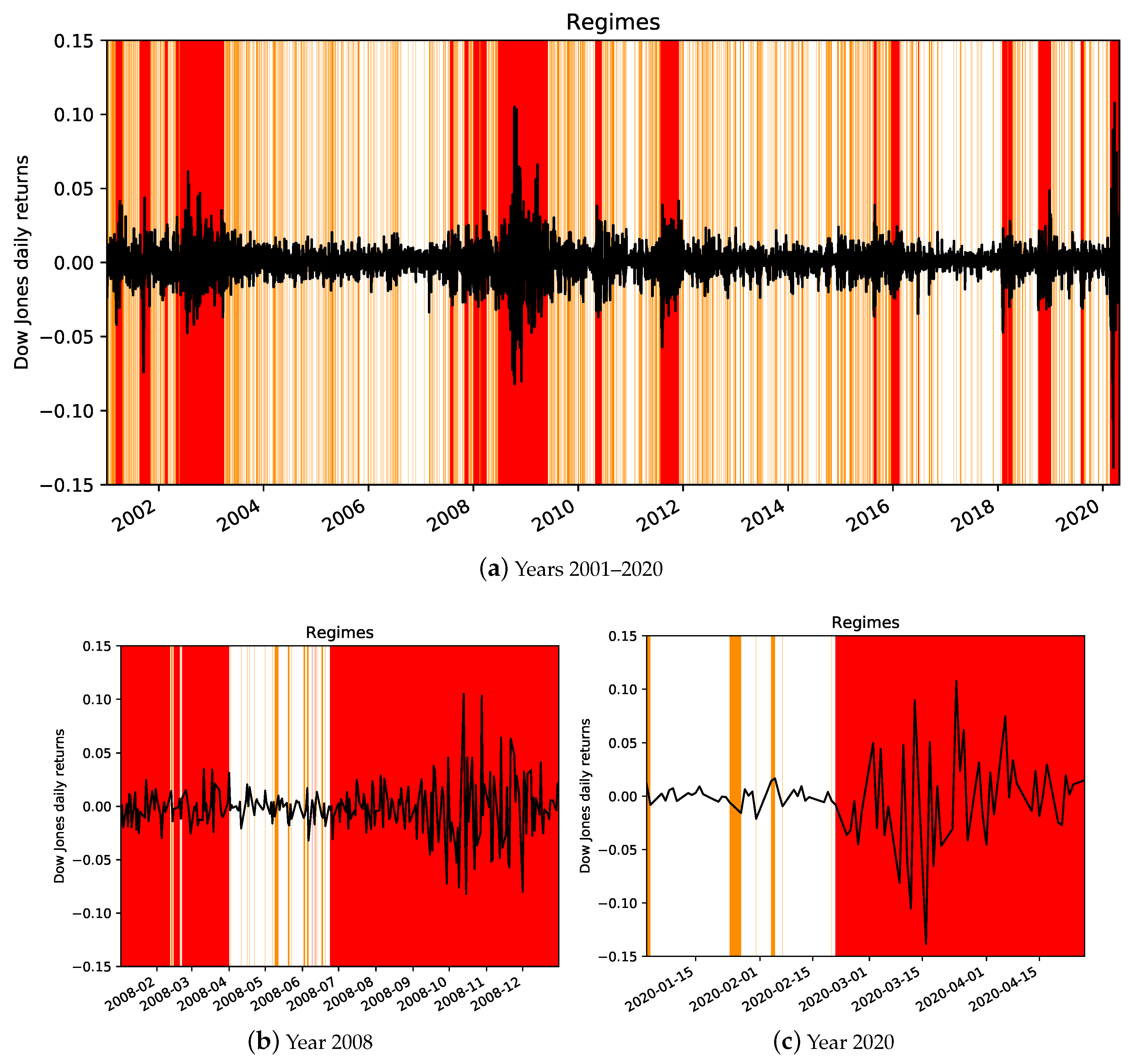
4.3. Analysis of Robustness

In this section, we provide an analysis of robustness of the proposed econometric model and, with this aim, we consider the DJIA index. The DJIA statistics, already reported in Table 3, are very close to the S&P 500 statistics. Furthermore, the DJIA index displays a high correlation with the S&P 500 index, and correlations similar to the ones of the S&P 500 index with the considered explanatory variables. As a consequence, for the DJIA index, we expect results similar to the ones of the S&P 500 for what concerns the multinomial logit model.

Table 5. 3-Regime Markov-switching models: estimated parameters for the Dow Jones Industrial Average index returns (2001–2020). AIC and BIC are the Akaike and Bayesian Information Criterion,  respectively.

Panel A: Estimated Parameters
	$\widehat{\mu }$	$\widehat{\sigma }$
Regime 0	0.001	0.005
Regime 1	−5.466$\times {10}^{-5}$	0.010
Regime 2	−0.001	0.022
Log-Likelihhod	15,861.07
AIC	−31,716.14
BIC	−31,671.21
Panel B: Transition Probabilities
	Regime 0	Regime 1	Regime 2
Regime 0	0.643	0.355	0.002
Regime 1	0.485	0.504	0.011
Regime 2	0.004	0.019	0.977

reports the estimated parameters for the returns of the DJIA index for the period of 4 January 2001 to 28 April 2020. As in the case of the S&P 500 returns, the three regimes identified for the DJIA index returns can be given the interpretation of tranquil, volatile, or turbulent regimes, respectively. In this case, the probability of permanence in the tranquil regime is approximately equal to $64\%$ and in the volatile regime is approximately $50\%$, whereas the probability of permanence in the turbulent regime is almost equal to $98\%$. These probabilities are different from the ones registered by the S&P 500 index, while a similarity is given by the probability of moving directly from the tranquil to the turbulent regime (or vise versa). Indeed, they are very close to zero, even if they are not negligible. A further difference between the two considered indexes is relative to the transition probability from the tranquil regime to the volatile one, which in the DJIA case is equal to $35.5\%$. By contrast, the transition probability equals $48.5\%$.

As before, we use the algorithm of Kim (1994) to derive smoothed probabilities, $P({ϵ}_t=j|{\Omega }_T;\theta )$, which are then used to determine whether a given day belongs to the tranquil, volatile, or turbulent regimes. Figure 2 plots the different regimes based on smoothed probabilities, together with the time series plots, for the DJIA index, while Panel (b) and Panel (c) zoom in on the years 2008 and 2020, respectively.

In

Table 6. Percentage of time spent by the Dow Jones Industrial Average index in each regime: ratio between number of days in regime i and number of days in the whole period.

Period	Tranquil	Volatile	Turbulent
2001–2020	58.69%	20.57%	20.74%
2008	13.83%	9.49%	76.68%
2020	31.25%	11.25%	57.50%

, we report the percentage of time spent in each one of the three considered regimes. We observe that during the entire period 2001–2020, the most frequent regime for the DJIA index is the tranquil one, as it is for the S&P 500 index, but when considering the year in which the subprime financial crisis peaked (2008) and the year the COVID-19 pandemic started (2020), the most frequent regime for the DJIA index is always the turbulent one (we recall that in the S&P 500 case in year 2008 the most frequent regime was the volatile one). Furthermore, while in the S&P 500 case the volatile regime has been more frequent than the tranquil one during the year of the peak of the subprime crisis and the four months of the COVID-19 crisis, the opposite happens in the DJIA case. If we focus on the entire 2001–2020 period, the frequency of the turbulent regime is about 10% for the S&P 500 index and close to 21% for the DJIA index.

Table 7. Estimated parameters for the multinomial logit models to explain regimes for the Dow Jones Industrial Average index. Regimes are identified by smoothed probabilities based on the estimated 3-regime Markov switching models. ‘***’, ‘**’, and ‘*’ denote significance at the 1%, 5%, and 10% levels, respectively.

	Estimate	Std. Error	z-Value	p-Value
Regime 1: (intercept)	−1.069	0.037	−28.514	<2.2$\times {10}^{-16}$ ***
Regime 2: (intercept)	−1.044	0.037	−28.243	<2.2$\times {10}^{-16}$ ***
Regime 1: VIX	0.020	0.005	3.695	2.2$\times {10}^{-4}$ ***
Regime 2: VIX	0.048	0.005	9.034	<2.2$\times {10}^{-16}$ ***
Regime 1: GOLD	0.008	0.035	0.222	0.824
Regime 2: GOLD	0.050	0.035	1.414	0.157
Regime 1: CL1	−0.029	0.015	−1.914	0.056 *
Regime 2: CL1	−0.042	0.014	−2.959	0.003 ***
Regime 1: DXY	0.050	0.080	0.633	0.527
Regime 2: DXY	0.037	0.079	0.467	0.640

reports the estimated parameters of the multinomial logit model for the DJIA index. As in the S&P 500 index, the estimated intercepts are negative in both the equations for the volatile and the turbulent regimes. Furthermore, returns associated with the VIX index are characterized by a positive sign in the equation of both the volatile and turbulent regimes and the variable is statistically significant for both regimes. Differently from the S&P case, in the turbulent regime, the coefficient associated with gold and the coefficient associated to the US dollar index are still positive but not statistically significant, while in the volatile regime the WTI oil coefficient is still negative but significant. Finally, it is worth mentioning that, for both the indexes, the coefficient associated with the WTI oil is negative and statistically significant at different levels.

5. Conclusions

In this paper, we have analyzed the dynamics of the S&P 500 index during the period 2001–2020, which comprises the two most recent financial crises: the COVID-19 pandemic and the subprime mortgage crisis. We used a three-regime switching model and shown that the three states of the underlying Markov chain can be interpreted as tranquil, volatile, and turbulent regimes. We show that for the considered 20-year period, the most frequent regime is the tranquil one, followed by the volatile one. Furthermore, for the year in which the subprime mortgage crisis peaked, the most frequent regime is the volatile one, while for the year in which COVID-19 pandemic began, the dominant regime is the turbulent one. As a comparison, we have estimated the same model to the returns of the Dow Jones Industrial Average index and documented that, in this case, the tranquil regime is dominant during the entire period, while during the two crisis peaks the most frequent regime was the turbulent one, followed by the tranquil one.

Using a multinomial logit model to describe the probabilities of volatile or turbulent spells, we found that, in the case of the S&P 500 index, the VIX index has some explanatory power for both the volatile and the turbulent regimes, while gold, WTI oil, and the dollar index are only significant in the equation for the turbulent regime. To further test the model applicability, we provided an additional analysis considering the Dow Jones Industrial Average index. We found that, for instance, differently from the S&P case, both in the volatile and turbulent regime, the gold and the US dollar indices have no explanatory power. On the contrary, the VIX index presents a high explanatory power for both regimes.

The methodology and findings in the present paper could be useful for both investors and regulators to assess and predict the probability that the market will experience volatile or turbulent regimes. Starting from this contribution, future studies will propose to use more sophisticated models, like regime switching models with jump components or stochastic volatility models, to name just a few, in order to test if they may help draw more detailed findings.

References

1. Algieri, Bernardina, Matthias Kalkuhl, and Nicolas Koch. 2017. A tale of two tails: Explaining extreme events in financialized agricultural markets. Food Policy 69: 256–69. [Google Scholar] [CrossRef]
2. Bae, Kee-Hong, G. Andrew Karolyi, and René M. Stulz. 2003. A new approach to measuring financial contagion. Review of Financial Studies 16: 717–63. [Google Scholar] [CrossRef]
3. Banerji, Gunjan. 2020. Traders Bet on Falling “Fear Gauge”. The Wall Street Journal. Available online: https://www.wsj.com/articles/traders-bet-on-falling-fear-gauge-11584466439 (accessed on 13 May 2020).
4. Bartash, Jeffry. 2020. The Record Number of People Applying for Jobless Benefits Is Even Worse Than It Looks. MarketWatch. Available online: https://www.marketwatch.com/story/the-record-number-of-people-applying-for-jobless-benefits-is-even-worse-than-it-looks-2020-05-07 (accessed on 13 May 2020).
5. Baur, Dirk. G., and Brian. M. Lucey. 2010. Is gold a hedge or a safe haven? An analysis of stocks, bonds and gold. Financial Review 45: 217–29. [Google Scholar] [CrossRef]
6. Black, Fischer, and Myron Scholes. 1973. The pricing of options and corporate liabilities. Journal of Political Economy 81: 637–59. [Google Scholar] [CrossRef] [Green Version]
7. Candelon, Bertrand, Jan Piplack, and Stefan Straetmans. 2008. On measuring synchronization of bulls and bears: The case of East Asia. Journal of Banking and Finance 32: 1022–35. [Google Scholar] [CrossRef]
8. Center of Hellenic Studies. 2008. The State of the Nation’s Housing. Joint Center for Housing Studies of Harvard University. Available online: http://www.jchs.harvard.edu/sites/jchs.harvard.edu/files/son2008.pdf (accessed on 13 May 2020).
9. Charles, Amelie, and Olivier Darné. 2014. Large shocks in the volatility of the Dow Jones Industrial Average index: 1928–2013. Journal of Banking and Finance 43: 188–99. [Google Scholar] [CrossRef] [Green Version]
10. Chen, Shiu-Sheng. 2010. Predicting the bear stock market: Macroeconomic variables as leading indicators. Journal of Banking and Finance 33: 211–23. [Google Scholar] [CrossRef]
11. Chiang, Shu-Mei. 2012. The relationships between implied volatility indexes and spot indexes. Procedia—Social and Behavioral Sciences 57: 231–35. [Google Scholar] [CrossRef] [Green Version]
12. Christiansen, Charlotte, and Angelo Ranaldo. 2009. Extreme coexceedances in new EU member states’ stock markets. Journal of Banking & Finance 33: 1048–57. [Google Scholar]
13. Coakley, Jerry, and Ana-Maria Fuertes. 2006. Valuation ratios and price deviations from fundamentals. Journal of Banking and Finance 30: 2325–46. [Google Scholar] [CrossRef]
14. Croissant, Yves. 2018. mlogit: Multinomial Logit Models. R package version 0.3-0. Available online: https://CRAN.R-project.org/package=mlogit (accessed on 13 May 2020).
15. Gopinath, Gita. 2019. The Great Lockdown: Worst Economic Downturn Since the Great Depression. IMFBlog. Available online: https://blogs.imf.org/2020/04/14/the-great-lockdown-worst-economic-downturn-since-the-great-depression/ (accessed on 13 May 2020).
16. Giot, Pierre. 2005. Relationships Between Implied Volatility Indexes and Stock Index Returns. The Journal of Portfolio Management 31: 92–100. [Google Scholar] [CrossRef] [Green Version]
17. Greene, William H. 2018. Econometric Analysis, 8th ed. Harlow: Pearson. [Google Scholar]
18. Hamilton, James D. 1983. Oil and the macroeconomy since world war II. Journal of Political Economy 91: 228–48. [Google Scholar] [CrossRef]
19. Hamilton, James D. 1989. A new approach to the economic analysis of non-stationary time series. Econometrica 57: 357–84. [Google Scholar] [CrossRef]
20. Hamilton, James D. 1990. Analysis of time series subject to changes in regime. Journal of Econometrics 45: 39–70. [Google Scholar] [CrossRef]
21. Hamilton, James D. 1994. Time Series Analysis. Princeton: Princeton University Press. [Google Scholar]
22. Hamilton, James D. 2003. What is an oil shock? Journal of Econometrics 113: 363–98. [Google Scholar] [CrossRef]
23. Hauptmann, Johannes, Anja Hoppenkamps, Aleksey Min, Franz Ramsauer, and Rudi Zagst. 2014. Forecasting market turbulence using regime-switching models. Financial Markets and Portfolio Management 28: 139–64. [Google Scholar] [CrossRef]
24. Imbert, Fred. 2020. Dow Jumps More Than 250 Points to a Record. CNBC. Available online: https://www.cnbc.com/2020/02/12/us-futures-point-to-higher-open-after-stocks-hit-fresh-record-highs.html (accessed on 13 May 2020).
25. Kim, Chang-Jin. 1994. Dynamic linear models with Markov-switching. Journal of Econometrics 60: 1–22. [Google Scholar] [CrossRef]
26. Koch, Nicolas. 2014. Tail events: A new approach to understanding extreme energy commodity prices. Energy Economics 43: 195–205. [Google Scholar] [CrossRef]
27. Maheu, John M., and Thomas H. McCurdy. 2000. Identifying bull and bear markets in stock returns. Journal of Business and Economic Statistics 18: 100–12. [Google Scholar]
28. Martinez-Peria, Maria Soledad. 2002. A regime-switching approach to the study of speculative attacks: A focus on EMS crises. Empirical Economics 27: 299–334. [Google Scholar] [CrossRef]
29. McLean, Rob, Laura He, and Anneken Tappe. 2020. Dow Plunges 1000 Points, Posting Its Worst Day in Two Years as Coronavirus Fears Spike. CNN Business. Available online: https://edition.cnn.com/2020/02/23/business/stock-futures-coronavirus/index.html (accessed on 13 May 2020).
30. Munich Re. 2020. Quarterly Statement: Low Quarterly Profit Due to High COVID-19-Related Losses. Available online: https://www.munichre.com/content/dam/munichre/mrwebsiteslaunches/2020-q1/MunichRe-Quarterly-Statement-1-2020_en.pdf/_jcr_content/renditions/original./MunichRe-Quarterly-Statement-1-2020_en.pdf (accessed on 13 May 2020).
31. Pape, Katharina, Dominik Wied, and Pedro Galeano. 2016. Monitoring multivariate variance changes. Journal of Empirical Finance 39: 54–68. [Google Scholar] [CrossRef] [Green Version]
32. Partington, Richard, and Graeme Wearden. 2020. Global Stock Markets Post Biggest Falls Since 2008 Financial Crisis. The Guardian. Available online: https://www.theguardian.com/business/2020/mar/09/global-stock-markets-post-biggest-falls-since-2008-financial-crisis (accessed on 13 May 2020).
33. Perez-Quiros, Gabriel, and Allan Timmermann. 2000. Firm size and cyclical variations in stock returns. Journal of Finance 55: 1229–62. [Google Scholar] [CrossRef]
34. R Core Team. 2019. R: A Language and Environment for Statistical Computing. Vienna: R Foundation for Statistical Computing, Available online: https://www.R-project.org/ (accessed on 13 May 2020).
35. Roubaud, David, and Mohamed Arouri. 2018. Oil prices, exchange rates and stock markets under uncertainty and regime-switching. Finance Research Letters 27: 28–33. [Google Scholar] [CrossRef]
36. Sanchez-Espigares, Josep, and Alberto Lopez-Moreno. 2018. MSwM: Fitting Markov Switching Models. R package version 1.4. Available online: https://CRAN.R-project.org/package=MSwM (accessed on 13 May 2020).
37. Schwert, G. William. 2011. Stock Volatility during the Recent Financial Crisis. European Financial Management 17: 789–805. [Google Scholar] [CrossRef]
38. Schich, Sebastian. 2010. Insurance companies and the financial crisis. OECD Journal: Financial Market Trends 2009: 121–51. [Google Scholar] [CrossRef]
39. The Economist. 2008. A helping hand to homeowners. Available online: https://www.economist.com/finance-and-economics/2008/10/23/a-helping-hand-to-homeowners (accessed on 13 May 2020).
1
To make the contents of this paper more accessible to non-economic readers, Table A1 in the Appendix A describes all the economic indicators and acronyms we use throughout the paper.
2
See Martinez-Peria (2002) for previous applications of regime switching models.