Article

Gerber–Shiu Function in a Class of Delayed and Perturbed Risk Model with Dependence

School of Economics, University of Johannesburg, Johannesburg 2006, South Africa
*
Author to whom correspondence should be addressed.
Risks 2020, 8(1), 30; https://doi.org/10.3390/risks8010030
Submission received: 20 February 2020 / Revised: 7 March 2020 / Accepted: 12 March 2020 / Published: 17 March 2020

Abstract

:
This paper considers the risk model perturbed by a diffusion process with a time delay in the arrival of the first two claims and takes into account dependence between claim amounts and the claim inter-occurrence times. Assuming that the time arrival of the first claim follows a generalized mixed equilibrium distribution, we derive the integro-differential Equations of the Gerber–Shiu function and its defective renewal equations. For the situation where claim amounts follow exponential distribution, we provide an explicit expression of the Gerber–Shiu function. Numerical examples are provided to illustrate the ruin probability.

1. Introduction

Financial institutions and insurers manage large amounts of capital and failure to properly estimate the risk of ruin can result in serious financial consequences. To this end, researchers have constructed a variety of models to study and predict the possible ruin time, the ruin probability, the claim outcomes, and other useful risk metrics. One can cite the aggregate claims models, the Sparre Andersen model, and many others. With these models, insurers are able to price and estimate the reserve and the ruin related quantities. One very valuable analytical tool to understanding the event of ruin is the Gerber–Shiu discounted penalty function (Gerber and Shiu 1998). This penalty function acts as a unified means of identifying ruin-related quantities, which may be instrumental in understanding the vulnerability of an insurance institution (Cheung and Feng 2013; Landriault and Willmot 2008; Lin and Willmot 2000; Pavlova and Willmot 2004; Schmidli 2010; Willmot 2007; Zhang et al. 2009; Zou and Xie 2012).
In the actuarial literature, the Gerber–Shiu function satisfies a defective renewal equation in the ordinary Sparre Andersen model. Due to the unrealistic nature of the model’s basic assumption of independence and identical distribution for the claim inter-arrival time, extensions to that model have been made. Consequently, extensions to the Gerber–Shiu function in the delayed renewal model have also been made. For example, ((Willmot 2004; Willmot and Dickson 2003) considered the case where the first inter claim time is assumed to follow a possibly different density than the common density of the subsequent inter-claims times. (Cheung et al. 2010) considered the Gerber–Shiu function in a more general settings. In particular, (Cai 2007; Cai et al. 2009; Zhou and Cai 2009) generalized a Gerber–Shiu function to a more general cost function.
On the central problem of risk in the insurance industry, that of estimating the probability of ruin, a lot of work has been done. (Dufresne and Gerber 1991) took the classical model of collective risk theory and added a diffusion process to the compound Poisson model. Then, they showed that the probabilities of ruin (by oscillation or by a claim) satisfy certain defective renewal Equations and that the convolution formula for the probability of ruin can be derived and interpreted in terms of the record highs of the aggregate loss process. (Wang 2001) worked on a decomposition of the ruin probability for the risk process perturbed by diffusion. (Tsai and Willmot 2002) considered the surplus process of the classical continuous time risk model assuming independent diffusion (Wiener) process. They generalized the defective renewal equation for the expected discounted function of a penalty at the time of ruin in (Gerber and Landry 1998). (Gao and Wu 2014) worked on the Gerber–Shiu discounted penalty function in a risk model with two types of delayed-claims and random income. They developed a new delayed model with random premium income and two types of by-claims, and then derived an integral system of equations for the Gerber–Shiu discounted penalty function and explicit solution of the Laplace transform of the discounted penalty function. They proved that the discounted penalty function satisfies a defective renewal equation and obtained an explicit result of the ruin probability under the exponential distribution. (Schmidli 2014) studied the gerber–shiu functions with an application. (Zhang and Yang 2011) worked on Gerber–Shiu analysis in a perturbed risk model with dependence between claim sizes and inter-claim times, where they also considered that the compound Poisson risk model is perturbed by a Brownian motion. (Lee and Willmot 2014) worked on the moments of the time to ruin in dependent Sparre Andersen models with emphasis on Coxian inter-claim times.
This paper takes the results of (Zhang and Yang 2011) and incorporates the delay in the arrival of the first two claim arrival times. The objective of this paper is to generalize (Zhang and Yang 2011) results to the case of the delayed renewal risk model with a generalized mixed equilibrium first claim time, first introduced by (Willmot 2004), and to derive the associated ruin probabilities. One justification of the delay renewal risk model is from observations within the car insurance industries. For instance, if there has been a long waiting time before a claim, the next inter-arrival time can be long, as well, because the policyholders are potentially “good drivers” or the reverse could be obtained, where some policyholders only start to use their cars a long time after purchasing them. Then, claims would suddenly arrive more frequently after a long silence.
The paper is structured as follows. In Section 2, the risk model is presented. In Section 3, we derive the equation for the Lundberg adjustment coefficient and its solutions. Section 4, Section 5 and Section 6 deal with the integro-differential equations, the Laplace transform, and the defective renewal equations, respectively. Representations of the solutions of the afore-mentioned equations are followed by numerical examples to illustrate the theory.

2. Risk Model

2.1. Definition of the Risk Model

We consider the following delay renewal risk process perturbed by an independent diffusion process. The delay renewal risk model used in this section is similar to the one proposed in (Willmot 2004). The surplus process at time t is:
U t = u + c t + σ B t i = 1 N t d X i , t 0 ,
where u is the initial surplus and c is the rate at which premiums are received per unit of time. N t d denotes the delayed renewal process, N t is the ordinary renewal process, and σ B t represents the diffusion process accounting for the perturbation that may arise from the market or due to model error. We denote by V i the time between the ( i 1 ) th and the ith claim for i = 2 , 3 ,
The assumptions of the model are summarized in the following:
  • the time arrival of the first claim V 1 has density function given by:
    f V 1 ( t ) = q λ 1 e λ 1 t + ( 1 q ) e λ 1 t t f V 2 ( y ) d y 0 e λ 1 y F ¯ V 2 ( y ) d y ,
where 0 q 1 , λ 1 > 0 , and the inter- occurrence time from the second claim V 2 has the density function f V 2 with survival function F ¯ V 2 .
Clearly, V 1 is a mixture of two random variables W i , i = 1 , 2 with density functions given by f W 1 ( t ) = λ 1 e λ 1 t   and   f W 2 ( t ) = e λ 1 t t f V 2 ( y ) d y 0 e λ 1 y F ¯ V 2 ( y ) d y , t 0 , with weights q and 1 q .
As in (Willmot 2004), the motivation for this particular choice of the generalized mixed-equilibrium distribution is two-fold. First, when q = 0 , f V 1 is a generalized equilibrium distribution. The stationary or equilibrium renewal risk model is a special case of the delayed renewal risk model where the time until the first claim has an equilibrium distribution different from the other inter-claim times’ distribution. The motivation of the equilibrium distribution is that it is the limiting distribution of the time until the next claim occurs. Second, when q = 1 , V 1 is exponentially distributed, which is an intriguing choice for the time until the first claim occurs. In particular, note that, if the duration between the last claim before time 0 and the first claim after time 0 is exponential, then the (conditional) distribution at time 0 of the time until the first claim after 0 has the same exponential density, regardless of when the last claim before 0 occurred, as follows from the memoryless property of the exponential distribution.
  • The time between the second and the third claim, V 2 , is exponentially distributed with parameter λ 2 ;
  • V i , i = 1 , 2 , are independent;
  • the subsequent claims inter-occurrence times { V i } i = 3 are exponentially distributed with parameter λ , i.e., V i V e x p ( λ ) , i = 3 , ;
  • { X i } i = 1 are independent and { X i } i = 3 are distributed as the generic X;
  • X i and V i are dependent and jointed by FGM copulas with parameter ( η i ) i = 1 , 2 , such that η i = η for i = 3 , ;
  • { ( X i , V i ) , i = 1 , 2 , } are mutually independent; and
  • the standard Brownian motion ( B t ) t 0 is independent of the aggregate claim process.

2.2. The Dependence

We introduce a specific structure of dependence based on the Farlie–Gumbel–Morgenstern (FGM) copula. While there are many copula families, the advantage of using the FGM copula and its generalizations lies in its mathematical manageability. As illustrated in (Cossette et al. 2010), it models the dependence structure between the claim amounts and their occurrence times such as catastrophic claims. Even if the FGM copula introduces only light dependence, it admits positive as well as negative dependence between a set of random variables and includes the independence copula when its parameter is zero. It is also known that the FGM copula is a Taylor approximation of order one of the Frank copula, Ali–Milkhail–Haq copula and Plackett copula (see Nelsen 2006).
The joint cumulative distribution function (c.d.f.) of ( X i , V i ) , the ith claim and its occurrence time is
F ( X i , V i ) ( x , t ) = C η i F G M ( F X i ( x ) , F V i ( t ) ) = F X i ( x ) F V i ( t ) + η i F X i ( x ) F V i ( t ) ( 1 F X i ( x ) ) ( 1 F V i ( t ) ) ,
for ( x , t ) R + R + and where F X i and F V i are the marginal c.d.f. Recall that the density of the FGM copula is c η i F G M ( u , v ) = 1 + η i ( 1 2 u ) ( 1 2 v ) , i = 1 , 2 , 3   and   η 3 = η for ( u , v ) [ 0 , 1 ] [ 0 , 1 ] so that the joint probability density function (p.d.f) of ( X i , V i ) is
f ( X i , V i ) ( x , t ) = 2 u v C η i F G M ( F X i ( x ) , F V i ( t ) ) = f X i ( x ) f V i ( t ) c η i F G M ( F X i ( x ) , F V i ( t ) ) = f X i ( x ) f V i ( t ) + η i f X i ( x ) f V i ( t ) ( 1 2 F X i ( x ) ) ( 1 2 F V i ( t ) ) = f X i ( x ) f V i ( t ) + η i f V i ( t ) h i ( x ) ( 1 2 F V i ( t ) ) f ( X i , V i ) ( x , t ) = ( f X i ( x ) η i h i ( x ) ) f V i ( t ) + 2 η i h i ( x ) f V i ( t ) F ¯ V i ( t ) ,
where h i ( x ) = f X i ( x ) ( 1 2 F X i ( x ) ) , f X i , f V i are the density functions of X i and V i , respectively, and F ¯ V i is the survival function of V i . For simplicity, we have the following notations: f i : = f X i ; h i : = h X i ; i = 1 , 2 ; f : = f X ; h : = h X , i = 1 , 2 .
Remark 1.
In this model, the risk process becomes ordinary renewal risk model after the occurrence of the second claim. Therefore, we call the whole model a second-order delayed renewal risk model (or risk model of Type II). After the occurrence of the first claim, the whole process becomes a first-order delayed renewal risk model (or of Type I) and then an ordinary renewal risk model.

3. Generalized Lundberg-Type Equation

In this section, we introduce a generalized version of the Lundberg equation for the risk process and analyze the existence of its roots. Let us define the Gerber–Shiu function by
m d ( u ) = E e δ τ w ( U τ , | U τ | ) I ( τ < ) | U ( 0 ) = u ,
where τ is the time of ruin (i.e., the first time the surplus level falls bellow zero) and is defined mathematically as:
τ = inf { t > 0 : U t < 0 }   if   U t 0 t > 0 .
To guarantee that ruin is not a certain event, we assume that the following net profit condition holds E [ c V k X k ] > 0 with k = 1 , 2 , The Gerber–Shiu function m d can be decomposed as:
m d ( u ) = ϕ d ( u ) + ψ d ( u ) ,
where
ϕ d ( u ) = E e δ τ w ( U τ , | U τ | ) I ( τ < , U τ < 0 ) | U ( 0 ) = u ,
ψ d ( u ) = E e δ τ w ( U τ , | U τ | ) I ( τ < , U τ = 0 ) | U ( 0 ) = u .
This decomposition can be explained by the fact that if the ruin occurs it can be caused either by oscillations or by claims. ϕ d , ψ d (respectively, ϕ , ψ ) represent the Gerber–Shiu functions when ruin is caused by claims and by oscillations in the delayed renewal risk model of Type I (respectively, the Gerber–Shiu functions in the ordinary renewal risk model).
Let us consider the sequence of the surplus at the nth claim such that
U n = u + c T n + σ B T n k = 1 N T n d X k ,
where T n = k = 1 n V k is the time occurrence of the nth claim. By the properties of Brownian motion (independent increment and stationary), we have the following equality in distribution,
U n = d u + k = 1 n ( c V k + σ B V k X k ) .
Let us determine s such that { e δ T n + s U n } n = 1 is a martingale.
By setting Z n = e δ T n + s U n , we have that Z n + 1 = Z n e δ V n + 1 + s ( c V n + 1 + σ B V n + 1 X n + 1 ) . The martingale condition is satisfied if
E [ e δ V n + 1 + s ( c V n + 1 + σ B V n + 1 X n + 1 ) ] = 1 .
Let us denote L ( s ) = E [ e δ V + s ( c V + σ B V X ) ] . The generalized Lundberg equation associated with the risk model in n 3 is given by the following ordinary Lundberg equation
L ( s ) = 1 ,
where
L ( s ) = 0 0 E [ e δ t + s ( c t + σ B t x ) ] f ( X , V ) ( x , t ) d x d t = 0 0 e ( δ s c σ 2 s 2 2 ) t s x f ( X , V ) ( x , t ) d x d t .
Substituting Equation (3) into Equation (8), one gets
L ( s ) = 2 λ [ f ˜ ( s ) η h ˜ ( s ) ] σ 2 A 1 ( s ) 4 λ η h ˜ ( s ) σ 2 A 2 ( s ) ,
with
A 1 ( s ) = s 2 + 2 c σ 2 s 2 ( λ + δ ) σ 2 , A 2 ( s ) = s 2 + 2 c σ 2 s 2 ( 2 λ + δ ) σ 2 ,
and f ˜ , h ˜ the Laplace transforms of f   and   h , i.e., f ˜ ( s ) = 0 e s x f ( x ) d x .
By the Rouché theorem and analogously to Propositions 1 and 2 of (Chadjiconstantinidis and Vrontos 2014), Equation (7) has exactly two roots in the the right complex plane, say ρ 1 , ρ 2 , such that R e ( ρ i ) > 0 and for δ = 0 one root is null.

4. Results

4.1. Integro-Differential Equation

In this section, we derive the integro-differential Equations that satisfy the Gerber–Shiu functions when ruin is caused by claims and by oscillations. We start with the first-order delayed and perturbed risk model (Type I), a model such that after the first claim the process becomes ordinary. In this case, the occurrence time of the first claim is exponentially distributed with parameter λ 2 , and the process becomes ordinary with claim inter-occurrence time following exponential distribution with parameter λ . Then, we move to the second-order delayed and perturbed risk model (Type II) where the time occurrence of the first claim follows the distribution given in Equation (2) and the time until the second claim is exponentially distributed with parameter λ 2 . Recall that, after the first claim, it behaves as the first-order delayed renewal risk model (Type I) before becoming ordinary. Let
σ f 2 ( u ) = 0 u ϕ ( u x ) f 2 ( x ) d x + w f 2 ( u ) ; w f 2 ( u ) = u w ( u , x u ) f 2 ( x ) d x ; σ h 2 ( u ) = 0 u ϕ ( u x ) h 2 ( x ) d x + w h 2 ( u ) ; w h 2 ( u ) = u w ( u , x u ) h 2 ( x ) d x ; σ f = lim f 2 f σ f 2 ; σ h = lim h 2 h σ f 2 ; w f = lim f 2 f w f 2 ; w h = lim h 2 h w h 2 ;
P 1 ( s ) = s 2 + 2 c σ 2 s 2 ( λ 2 + δ ) σ 2 ; P 2 ( s ) = s 2 + 2 c σ 2 s 2 ( 2 λ 2 + δ ) σ 2 .
Setting D : = d d u ( · ) , D 2 : = d 2 d u 2 ( · ) , I   the   identity   operator , we define the following differentiation operators:
P 1 ( D ) = D 2 + 2 c σ 2 D 2 ( λ 2 + δ ) σ 2 I , P 2 ( D ) = D 2 + 2 c σ 2 D 2 ( 2 λ 2 + δ ) σ 2 I , A 1 ( D ) = lim λ 2 λ P 1 ( D ) , A 2 ( D ) = lim λ 2 λ P 2 ( D ) .
Theorem 1.
Under the assumptions of the first-order delayed and perturbed risk model (Type I) defined in Equation (1), the Gerber–Shiu function ϕ d defined in Equation (5) when the ruin is caused by claims satisfies the following integro-differential equation,
P 1 ( D ) P 2 ( D ) ( ϕ d ) ( u ) = 2 λ 2 σ 2 P 2 ( D ) ( σ f 2 ( u ) η 2 σ h 2 ( u ) ) 4 λ 2 η 2 σ 2 P 1 ( D ) ( σ h 2 ( u ) ) ,
with the boundary conditions
ϕ d ( 0 ) = 0 , ϕ d ( 0 ) + 2 c σ 2 ϕ d ( 0 ) = 2 λ 2 σ 2 ( w f 2 ( 0 ) + η 2 w h 2 ( 0 ) ) .
In Equation (12), σ f 2 , σ h 2 defined in Equation (10) are functions of the ordinary Gerber–Shiu function ϕ which satisfies
A 1 ( D ) A 2 ( D ) ( ϕ ) ( u ) = 2 λ σ 2 A 2 ( D ) ( σ f ( u ) η σ h ( u ) ) 4 λ η σ 2 A 1 ( D ) ( σ h ( u ) ) .
Remark 2.
By letting λ 2 λ , f 2 f and η 2 η , Equation (12) reduces to the integro-differential Equation in the ordinary renewal risk model in Equation (14), which is the equation from Theorem 1 of (Zhang and Yang 2011).
Proof. 
Let Z t = c t σ B t and Z t ¯ = sup 0 s t { Z s } . The condition u Z t ¯ > 0 ensures that the ruin is not always caused by oscillation, i.e., the surplus process U t is not defined to be almost surely negative. Let us recall the Wiener–Hopf factorization theorem (Kyprianou 2006). Given an independent exponentially distributed random variable e a with mean 1 a , the random variables Z ¯ e a and Z ¯ e a Z e a are independent and exponentially distributed. Let a 1 , a 2 be the corresponding rates.
E [ e s Z e a ] = E [ e s ( Z ¯ e a Z e a ) s Z ¯ e a ] = E [ e s ( Z ¯ e a Z e a ) ] E [ e s Z ¯ e a ] = a 1 a 1 + s a 2 a 2 s ,
and
E [ e s Z e a ] = 0 E [ e s Z t ] f e a ( t ) d t = 0 e t ( c s + σ 2 s 2 2 ) f e a ( t ) d t = a a c s σ 2 s 2 2 .
The roots of a c s σ 2 s 2 2 are a 1 and a 2 , with a 1 = c σ 2 + c 2 σ 4 + 2 a σ 2 , a 2 = c σ 2 + c 2 σ 4 + 2 a σ 2 .
We now derive the expression of the Gerber–Shiu function by conditioning on the occurrence of claims and taking into account the fact that ruin may occur or not.
ϕ d ( u ) = E [ e V 2 δ E [ w ( u Z V 2 , X 2 u + Z V 2 ) 1 ( X 2 > u Z V 2 , Z V 2 ¯ < u ) | ( V 2 , X 2 ) ] ] + E [ e V 2 δ E [ ϕ ( u Z V 2 X 2 ) 1 ( X 2 < u Z V 2 , Z V 2 ¯ < u ) | ( V 2 , X 2 ) ] ] = 0 u u y e δ t [ w ( u y , x ( u y ) ) ] P [ ( Z t d y , Z ¯ t < u ) ] f ( V 2 , X 2 ) ( t , x ) d x d t + 0 u 0 u y e δ t ϕ ( u y x ) ] P [ ( Z t d y , Z ¯ t < u ) ] f ( V 1 , X 1 ) ( t , x ) d x d t = u u y w ( u y , x ( u y ) ) p ( u , y , x ) d x d y + u 0 u y ϕ ( u y x ) ] p ( u , y , x ) d x d y .
The measure p is defined by:
p ( u , d y , d x ) = p ( u , d y , d x | λ 2 , η 2 ) = 0 [ λ 2 e ( δ + λ 2 ) t ( f 2 ( x ) η 2 h 2 ( x ) ) ) + 2 η 2 λ 2 e ( 2 λ 2 + δ ) t h 2 ( x ) ] P [ ( Z t d y Z ¯ t < u ) ] d x d t = λ 2 λ 2 + δ ( f 2 ( x ) η 2 h 2 ( x ) ) ) P [ ( Z e ( λ 2 + δ ) d y , Z ¯ e ( λ 2 + δ ) < u ) ] + 2 η 2 λ 2 2 λ 2 + δ e ( 2 λ 2 + δ ) t h 2 ( x ) ] P [ ( Z e ( 2 λ 2 + δ ) d y , Z ¯ e ( 2 λ 2 + δ ) < u ) ] .
Because
P [ ( Z e a d y , Z ¯ e a < u ) ] = m a x ( 0 , y ) u P [ ( Z ¯ e a Z e a Z ¯ e a ) d y , Z ¯ e a d x ) ] = m a x ( 0 , y ) u P [ ( Z ¯ e a Z e a x d y , Z ¯ e a d x ) ] = m a x ( 0 , y ) u a 1 a 2 e ( a 1 + a 2 ) x + a 2 y d x d y = a 1 a 2 a 1 + a 2 e ( a 1 + a 2 ) m a x ( 0 , y ) + a 2 y e ( a 1 + a 2 ) u + a 2 y d y ,
applying Equation (17) to Equation (16), we have: for 0 y < u ,
p ( u , y , x ) = p ( u , y , x | λ 2 , η 2 ) = λ 2 α 1 α 2 ( λ 2 + δ ) ( α 1 + α 2 ) ( e α 1 y e ( α 1 + α 2 ) u + α 2 y ) ( f 2 ( x ) η 2 h 2 ( x ) ) + 2 η 2 λ 2 β 1 β 2 ( 2 λ 2 + δ ) ( β 1 + β 2 ) ( e β 1 y e ( β 1 + β 2 ) u + β 2 y ) ( h 2 ( x ) ) ,
and for y < 0
p ( u , y , x ) = p ( u , y , x | λ 2 , η 2 ) = λ 2 α 1 α 2 ( λ 2 + δ ) ( α 1 + α 2 ) ( e α 2 y e ( α 1 + α 2 ) u + α 2 y ) ( f 2 ( x ) η 2 h 2 ( x ) ) + 2 η 2 λ 2 β 1 β 2 ( 2 λ 2 + δ ) ( β 1 + β 2 ) ( e β 2 y e ( β 1 + β 2 ) u + β 2 y ) ( h 2 ( x ) ) ,
where
α 1 = c σ 2 + 2 ( λ 2 + δ ) σ 2 + c 2 σ 4 , α 2 = c σ 2 + 2 ( λ 2 + δ ) σ 2 + c 2 σ 4 , β 1 = c σ 2 + 2 ( 2 λ 2 + δ ) σ 2 + c 2 σ 4 , β 2 = c σ 2 + 2 ( 2 λ 2 + δ ) σ 2 + c 2 σ 4 .
Substituting p ( u , y , x ) into Equation (15), setting v = u y , and rearranging, we get
ϕ d ( u ) = λ 2 α 1 α 2 ( 2 λ 2 + δ ) ( α 1 + α 2 ) 0 u e α 1 ( u v ) ( σ f 2 ( v ) η 2 σ h 2 ( v ) ) d v 0 e α 1 u α 2 v ( σ f 2 ( v ) η 2 σ h 2 ( v ) ) d v + u e α 2 ( u v ) ( σ f 2 ( v ) η 2 σ h 2 ( v ) ) d v + 2 η 2 λ 2 β 1 β 2 ( 2 λ 2 + δ ) ( β 1 + β 2 ) 0 u e β 1 ( u v ) σ h 2 ( v ) d v 0 e β 1 u β 2 v σ h 2 ( v ) d v + u e β 2 ( u v ) σ h 2 ( v ) d v .
Applying the operators P 1 ( D ) , P 2 ( D ) defined in Equation (11) (which can be re-written as P 1 ( D ) = ( D + α 1 I ) ( D α 2 I ) , P 2 ( D ) = ( D + β 1 I ) ( D β 2 I ) ) to Equation (20), we get the result (12). In Equation (20), we see that ϕ d ( 0 ) = 0 and by taking the first, the second derivative, and setting u = 0 leads to the boundary conditions. □
Let us
ζ f 2 ( u ) = 0 u ψ ( u x ) f 2 ( x ) d x ; ζ h 2 ( u ) = 0 u ψ ( u x ) h 2 ( x ) d x ; ζ f = lim f 2 f ζ f 2 , ζ h = lim h 2 h ζ h 2 .
Theorem 2.
Under the assumptions of the first-order delayed and perturbed risk model (Type I) defined in Equation (1), the Gerber–Shiu function ψ d defined in Equation (6) when the ruin is caused by oscillation satisfies the following integro-differential equation,
P 1 ( D ) P 2 ( D ) ( ψ d ) ( u ) = 2 λ 2 σ 2 P 2 ( D ) ( ζ f 2 ( u ) η 2 ζ h 2 ( u ) ) 4 λ 2 η 2 σ 2 P 1 ( D ) ( ζ h 2 ( u ) ) ,
with the boundary conditions,
ψ d ( 0 ) = 1 , ψ d ( 0 ) + 2 c σ 2 ψ d ( 0 ) = 2 ( λ 2 + δ ) σ 2 .
In Equation (22), ζ f 2 , ζ h 2 defined in Equation (21) are functions of the ordinary Gerber–Shiu function ψ, which satisfies
A 1 ( D ) A 2 ( D ) ( ψ ) ( u ) = 2 λ σ 2 A 2 ( D ) ( ζ f ( u ) η ζ h ( u ) ) 4 λ η σ 2 A 1 ( D ) ( ζ h ( u ) ) .
Remark 3.
By letting λ 2 λ , f 2 f and η 2 η , Equation (22) reduces to the integro-differential equation in the ordinary renewal risk model in Equation (24), which is the equation from Theorem 2 of (Zhang and Yang 2011).
Proof. 
Let τ u = inf { t 0 : Z t = u } ,
E [ e δ τ u 1 ( τ < V 2 ) ] = E [ e δ τ u E [ 1 ( τ u < V 2 ) ] | Z t ] = E [ e ( δ + λ 2 ) τ u ] = e α 1 u ,
using Formula (2.01) of (Borodin and Salminen 2002).
By conditioning on the fact that ruin caused by oscillation may occur or not before the first claim,
ψ d ( u ) = E [ e δ τ u 1 ( τ < V 2 ) ] + E [ e δ V 2 E [ ψ ( u Z V 2 X 2 ) 1 ( X 2 < u Z V 2 , Z V 2 ¯ < u ) | ( V 2 , X 2 ) ] ] = e α 1 u + 0 u 0 u y e δ t ψ ( u y x ) ] P [ ( Z t d y , Z ¯ t < u ) ] f ( V 1 , X 1 ) ( t , x ) d x d t = e α 1 u + u 0 u y ψ ( u y x ) p ( u , y , x ) d x d y .
In the same way as Theorem 1, we get the result. □
We are now able to determine the differential Equation of the defined risk process of Type II. Conditioning on the arrival of the first claim leads to the Type I risk process, which leads to the ordinary.
ϕ d ( u ) = E [ e δ V 1 E [ w ( u Z V 1 , X 1 u + Z V 1 ) 1 ( X 1 > u Z V 1 , Z V 1 ¯ < u ) | ( V 1 , X 1 ) ] ] + E [ e δ V 1 E [ ϕ d ( u Z V 1 X 1 ) 1 ( X 1 < u Z V 1 , Z V 1 ¯ < u ) | ( V 1 , X 1 ) ] ] = q E [ e δ W 1 E [ w ( u Z W 1 , X 1 u + Z W 1 ) 1 ( X 1 > u Z W 1 , Z W 1 ¯ < u ) | ( W 1 , X 1 ) ] ] + ( 1 q ) E [ e δ W 2 E [ w ( u Z W 2 , X 1 u + Z W 2 ) 1 ( X 1 > u Z W 2 , Z W 2 ¯ < u ) | ( W 2 , X 1 ) ] ] + q E [ e δ W 1 E [ ϕ d ( u Z W 1 X 1 ) 1 ( X 1 < u Z W 1 , Z W 1 ¯ < u ) | ( W 1 , X 0 ) ] ] + ( 1 q ) E [ e δ W 2 E [ ϕ d ( u Z W 2 X 1 ) 1 ( X 1 < u Z W 2 , Z W 2 ¯ < u ) | ( W 2 , X 1 ) ] ] , ϕ d ( u ) = : q ϕ 1 ( u ) + ( 1 q ) ϕ 2 ( u ) .
Then,
ϕ 1 ( u ) = E [ e δ W 1 E [ w ( u Z W 1 , X 1 u + Z W 1 ) 1 ( X 1 > u Z W 1 , Z W 1 ¯ < u ) | ( W 1 , X 1 ) ] ] + E [ e δ W 1 E [ ϕ d ( u Z W 1 X 1 ) 1 ( X 1 < u Z W 1 , Z W 1 ¯ < u ) | ( W 1 , X 1 ) ] ] = u u y w ( u y , x ( u y ) ) p ( u , y , x | λ 1 , η 1 ) d x d y + u 0 u y ϕ d ( u y x ) p ( u , y , x | λ 1 , η 1 ) d x d y .
Since we assume that V 2 is exponentially distributed with parameter λ 2 , the distribution of W 2 becomes:
f W 2 ( t ) = e λ 1 t t f V 2 ( y ) d y 0 e λ 1 y F ¯ V 2 ( y ) d y = ( λ 1 + λ 2 ) e ( λ 1 + λ 2 ) t , t 0 .
Thus,
ϕ 2 ( u ) = E [ e δ W 2 E [ w ( u Z W 2 , X 1 u + Z W 2 ) 1 ( X 1 > u Z W 2 , Z W 2 ¯ < u ) | ( W 2 , X 1 ) ] ] + E [ e δ W 2 E [ ϕ d ( u Z W 2 X 1 ) 1 ( X 1 < u Z W 2 , Z W 2 ¯ < u ) | ( W 1 , X 1 ) ] ] = u u y w ( u y , x ( u y ) ) p ( u , y , x | λ 1 + λ 2 , η 1 ) d x d y + u 0 u y ϕ d ( u y x ) p ( u , y , x | λ 1 + λ 2 , η 1 ) d x d y .
Therefore, the Hopf factorization theorem holds also in this case as in Theorem 1. Let
σ f 1 ( u ) = 0 u ϕ d ( u x ) f 1 ( x ) d x + w f 1 ( u ) , w f 1 ( u ) = u w ( u , x u ) f 1 ( x ) d x , σ h 1 ( u ) = 0 u ϕ d ( u x ) h 1 ( x ) d x + w h 1 ( u ) , w h 1 ( u ) = u w ( u , x u ) h 1 ( x ) d x ,
B 1 ( s ) = s 2 + 2 c σ 2 s 2 ( λ 1 + δ ) σ 2 , B 2 ( s ) = s 2 + 2 c σ 2 s 2 ( 2 λ 1 + δ ) σ 2 , B 1 e ( s ) = s 2 + 2 c σ 2 s 2 ( λ 1 + λ 2 + δ ) σ 2 , B 2 e ( s ) = s 2 + 2 c σ 2 s 2 ( 2 ( λ 1 + λ 2 ) + δ ) σ 2 .
Theorem 3.
Under the assumptions of the second-order delayed and perturbed risk model (Type II) defined in Equation (1), the Gerber–Shiu function ϕ d defined in Equation (5) when the ruin is caused by claims satisfies the following integro-differential equation,
B 1 ( D ) B 2 ( D ) B 1 e ( D ) B 2 e ( D ) ( ϕ d ) ( u ) + q 2 λ 1 σ 2 B 2 ( D ) B 1 e ( D ) B 2 e ( D ) + ( 1 q ) 2 ( λ 1 + λ 2 ) σ 2 B 1 ( D ) B 2 ( D ) B 2 e ( D ) ( σ f 1 ( u ) η 1 σ h 1 ( u ) ) + q 4 λ 1 η 1 σ 2 B 1 ( D ) B 1 e ( D ) B 2 e ( D ) + ( 1 q ) 4 ( λ 1 + λ 2 ) η 1 σ 2 B 1 e ( D ) B 1 ( D ) B 2 ( D ) ( σ h 1 ( u ) ) = 0 ,
with the boundary conditions
ϕ d ( 0 ) = 0 , ϕ d ( 0 ) + 2 c σ 2 ϕ d ( 0 ) = q 2 λ 1 σ 2 + ( 1 q ) 2 ( λ 1 + λ 2 ) σ 2 ( w f 1 ( 0 ) + η 1 w h 1 ( 0 ) ) .
In Equation (29), σ f 1 , σ h 1 defined in Equation (28) are functions of the Gerber–Shiu function ϕ d which satisfies Equation (12).
Proof. 
Since ϕ d ( u ) = q ϕ 1 ( u ) + ( 1 q ) ϕ 2 ( u ) , ϕ 1 , ϕ 2 defined in Equations (26) and (27), by proceeding as in Theorem 1, satisfy, respectively,
B 1 ( D ) B 2 ( D ) ( ϕ 1 ) ( u ) + 2 λ 1 σ 2 B 2 ( D ) ( σ f 1 ( u ) η 1 σ h 1 ( u ) ) + 4 λ 1 η 1 σ 2 B 1 ( D ) ( σ h 1 ( u ) ) = 0 ,
B 1 e ( D ) B 2 e ( D ) ( ϕ 2 ) ( u ) + 2 ( λ 1 + λ 2 ) σ 2 B 2 e ( D ) ( σ f 1 ( u ) η 1 σ h 1 ( u ) ) + 4 ( λ 1 + λ 2 ) η 1 σ 2 B 1 e ( D ) ( σ h 1 ( u ) ) = 0 .
Applying the operator q B 1 e ( D ) B 2 e ( D ) to Equation (31) added to the operator ( 1 q ) B 1 ( D ) B 2 ( D ) applied to Equation (32) leads to the result. The boundary conditions are obtained in the same way. □
Let
ζ f 1 ( u ) = 0 u ψ d ( u x ) f 1 ( x ) d x , ζ h 1 ( u ) = 0 u ψ d ( u x ) h 1 ( x ) d x .
Theorem 4.
Under the assumptions of the second-order delayed and perturbed risk model (Type II) defined in Equation (1), the Gerber–Shiu function ψ d defined in Equation (5) when the ruin is caused by oscillation satisfies the following integro-differential equation,
B 1 ( D ) B 2 ( D ) B 1 e ( D ) B 2 e ( D ) ( ψ d ) ( u ) + q 2 λ 1 σ 2 B 2 ( D ) B 1 e ( D ) B 2 e ( D ) + ( 1 q ) 2 ( λ 1 + λ 2 ) σ 2 B 1 ( D ) B 2 ( D ) B 2 e ( D ) ( ζ f 1 ( u ) η 1 ζ h 1 ( u ) ) + q 4 λ 1 η 1 σ 2 B 1 ( D ) B 1 e ( D ) B 2 e ( D ) + ( 1 q ) 4 ( λ 1 + λ 2 ) η 1 σ 2 B 1 e ( D ) B 1 ( D ) B 2 ( D ) ( ζ h 1 ( u ) ) = 0 ,
with the boundary conditions
ψ d ( 0 ) = 1 ; ϕ d ( 0 ) + 2 c σ 2 ϕ d ( 0 ) = q 2 ( λ 1 + δ ) σ 2 + ( 1 q ) 2 ( λ 1 + λ 2 + δ ) σ 2 .
In Equation (34), σ f 1 , σ h 1 defined in Equation (33) are functions of the Gerber–Shiu function ψ d which satisfies Equation (22).
Proof. 
As in the previous case of ϕ d , applying the same argument as in Theorem 2 leads to the result. Since τ u = inf { t 0 : Z t = u } ,
E [ e δ τ u 1 ( τ < V 1 ) ] = q E [ e δ τ u E [ 1 ( τ u < W 1 ) ] | Z t ] + ( 1 q ) E [ e δ τ u E [ 1 ( τ u < W 2 ) ] | Z t ] = q E [ e ( δ + λ 1 ) τ u ] + ( 1 q ) E [ e ( δ + λ 1 + λ 2 ) τ u ] , Thus   ψ d ( u ) = q ψ 1 ( u ) + ( 1 q ) ψ 2 ( u ) , ψ 1 ( u ) = E [ e ( δ + λ 1 ) τ u ] + u 0 u y ψ d ( u y x ) p ( u , y , x | λ 1 , η 1 ) d x d y , ψ 2 ( u ) = E [ e ( δ + λ 1 + λ 2 ) τ u ] + u 0 u y ψ d ( u y x ) p ( u , y , x | λ 1 + λ 2 , η 1 ) d x d y .
The result follows as in the proof of Theorem 3. □

4.2. Laplace Transform of the Gerber–Shiu Functions

Lemma 1.
The Laplace transform of ϕ d is given by
ϕ d ˜ ( s ) = 2 λ 2 σ 2 ( l 1 d ( s ) v 1 d ( s ) ) P 1 ( s ) P 2 ( s ) 2 λ σ 2 ( l 1 ( s ) v 1 ( s ) ) [ P 2 ( s ) ( f ˜ 2 ( s ) η 2 h ˜ 2 ( s ) ) + 2 η 2 P 1 ( s ) h ˜ 2 ( s ) ] P 1 ( s ) P 2 ( s ) [ A 1 ( s ) A 2 ( s ) + 2 λ σ 2 ( f ˜ ( s ) η h ˜ ( s ) ) A 2 ( s ) + 4 λ η σ 2 A 1 ( s ) h ˜ ( s ) ] ,
where
v 1 d ( s ) = P 2 ( s ) ( w ˜ f 2 ( s ) η 2 w ˜ f 2 ( s ) ) + 2 η 2 P 1 ( s ) h ˜ 2 ( s ) , v 1 ( s ) = lim λ 2 λ , f 2 f , η 2 η v 1 d ( s ) = A 2 ( s ) ( w ˜ f ( s ) η w ˜ f ( s ) ) + 2 η A 1 ( s ) h ˜ ( s ) , l 1 d ( s ) = σ 2 2 λ 2 ϕ ˜ d ( 0 ) ( s 2 + 2 c σ 2 s + 4 c 2 σ 4 2 ( 3 λ 2 + 2 δ ) σ 2 ) + 4 c σ 2 ϕ d ( 0 ) + ϕ ˜ d ( 0 ) + 2 c σ 2 ( w f 2 ( 0 ) + η 2 w h 2 ( 0 ) ) + σ f 2 ( 0 ) + η 2 σ h 2 ( 0 ) , l 1 ( s ) = σ 2 2 λ ϕ ˜ ( 0 ) ( s 2 + 2 c σ 2 s + 4 c 2 σ 4 2 ( 3 λ + 2 δ ) σ 2 ) + 4 c σ 2 ϕ ( 0 ) + ϕ ˜ ( 0 ) + 2 c σ 2 ( w f ( 0 ) + η w h ( 0 ) ) + σ f ( 0 ) + η σ h ( 0 ) .
Proof. 
0 e s u P 1 ( D ) P 2 ( D ) ( ϕ d ( u ) ) = ϕ ˜ d ( s ) P 1 ( s ) P 2 ( s ) ϕ d ( 0 ) 4 c 2 σ 4 2 ( 3 λ 2 + 2 δ ) σ 2 + 4 c σ 2 s + s 2 ϕ d ( 0 ) ( 4 c σ 2 + s ) ϕ d ( 0 ) .
2 λ 2 σ 2 0 e s u [ P 2 ( D ) ( σ f 2 ( u ) η 2 σ h 2 ( u ) ) + P 2 ( D ) ( σ h 2 ( u ) ) ] d u = 2 λ 2 σ 2 ϕ ˜ ( s ) [ P 2 ( s ) ( f ˜ 2 ( s ) η 2 h ˜ 2 ( s ) ) + 2 η 2 P 1 ( s ) h ˜ 2 ( s ) ] 2 λ 2 σ 2 [ P 2 ( w ˜ f 2 ( s ) η 2 w ˜ h 2 ( s ) ) + 2 η 2 P 1 ( s ) w ˜ h 2 ( s ) ] + 2 λ 2 σ 2 ( w f 2 ( 0 ) + η 2 w h 2 ( 0 ) ) ( s + 2 c σ 2 ) + 2 λ 2 σ 2 ( σ f 2 ( 0 ) + η 2 σ h 2 ( 0 ) ) .
Taking the Laplace transform of Equation (12) and using Equations (37) and (38) with the boundary conditions, we get
ϕ d ˜ ( s ) = 2 λ 2 σ 2 ( l 1 d ( s ) v 1 d ( s ) ) P 1 ( s ) P 2 ( s ) ϕ ˜ ( s ) P 2 ( s ) ( f ˜ 2 ( s ) η 2 h ˜ 2 ( s ) ) + 2 η 2 P 1 ( s ) h ˜ 2 ( s ) P 1 ( s ) P 2 ( s ) ,
where ϕ ˜ is obtained by taking the Laplace transform of (14) that is:
ϕ ˜ ( s ) = 2 λ σ 2 ( l 1 ( s ) v 1 ( s ) ) A 1 ( s ) A 2 ( s ) + 2 λ σ 2 ( f ˜ ( s ) η h ˜ ( s ) ) A 2 ( s ) + 4 λ η σ 2 A 1 ( s ) h ˜ ( s ) .
Substituting Equation (40) into Equation (39) leads to Equation (36). □
Lemma 2.
The Laplace transform of ϕ d is given by
ψ d ˜ ( s ) = ( l 2 d ( s ) v 2 d ( s ) ) P 1 ( s ) P 2 ( s ) 2 λ 2 σ 2 ( l 2 ( s ) v 2 ( s ) ) [ P 2 ( s ) ( f ˜ 2 ( s ) η 2 h ˜ 2 ( s ) ) + 2 η 2 P 1 ( s ) h ˜ 2 ( s ) ] P 1 ( s ) P 2 ( s ) [ A 1 ( s ) A 2 ( s ) + 2 λ σ 2 ( f ˜ ( s ) η h ˜ ( s ) ) A 2 ( s ) + 4 λ η σ 2 A 1 ( s ) h ˜ ( s ) ] ,
where
v 2 d ( s ) = s 3 + 4 c σ 2 s 2 + 4 c 2 σ 4 2 ( λ 2 + δ ) σ 2 , v 2 ( s ) = s 3 + 4 c σ 2 s 2 + 4 c 2 σ 4 2 ( λ + δ ) σ 2 , l 2 d ( s ) = ψ ˜ d ( 0 ) s 2 + 2 c σ 2 s + 4 c 2 σ 4 2 ( 3 λ 2 + 2 δ ) σ 2 + 4 c σ 2 ψ d ( 0 ) + ψ d ( 0 ) + 2 λ 2 σ 2 ( ζ f 2 ( 0 ) + η 2 ζ h 2 ( 0 ) ) , l 2 ( s ) = ψ ˜ ( 0 ) s 2 + 2 c σ 2 s + 4 c 2 σ 4 2 ( 3 λ + 2 δ ) σ 2 + 4 c σ 2 ψ ( 0 ) + ψ ( 0 ) + 2 λ σ 2 ( ζ f ( 0 ) + η ζ h ( 0 ) ) .
Proof. 
In the same way as the poof of Equation (36), we get the result. □
Lemma 3.
The Laplace transform of ϕ d is given by
ϕ ˜ d ( s ) = M ˜ 1 ( s ) + ϕ ˜ d ( s ) g ˜ 1 ( s ) ,
where ϕ ˜ d is given by Equation (36),
M ˜ 1 ( s ) = q 2 λ 1 σ 2 ( L 1 ( s ) V 1 ( s ) ) B 1 ( s ) B 2 ( s ) + ( 1 q ) 2 ( λ 1 + λ 2 ) σ 2 ( L 1 e ( s ) V 1 e ( s ) ) B 1 e ( s ) B 2 e ( s ) , g ˜ 1 ( s ) = q 2 λ 1 σ 2 B 2 ( s ) ( f ˜ 1 ( s ) η 1 h ˜ 1 ( s ) ) + 2 η 1 B 1 ( s ) h ˜ 1 ( s ) B 1 ( s ) B 2 ( s ) ( 1 q ) 2 ( λ 1 + λ 2 ) σ 2 B 2 e ( s ) ( f ˜ 1 ( s ) η 1 h ˜ 1 ( s ) ) + 2 η 1 B 1 e ( s ) h ˜ 1 ( s ) B 1 e ( s ) B 2 e ( s ) , V 1 ( s ) = B 2 ( s ) ( w ˜ f 1 ( s ) η 1 w ˜ f 1 ( s ) ) + 2 η 1 B 1 ( s ) h ˜ 1 ( s ) , L 1 ( s ) = σ 2 2 λ 1 ϕ ˜ 1 ( 0 ) ( s 2 + 2 c σ 2 s + 4 c 2 σ 4 2 ( 3 λ 1 + 2 δ ) σ 2 ) + 4 c σ 2 ϕ 1 ( 0 ) + ϕ ˜ 1 ( 0 ) + 2 c σ 2 ( w f 1 ( 0 ) ) + η 1 w h 1 ( 0 ) ) + σ f 1 ( 0 ) + η 1 σ h 1 ( 0 ) , V 1 e ( s ) = B 2 e ( s ) ( w ˜ f 1 ( s ) η 1 w ˜ f 1 ( s ) ) + 2 η 1 B 1 e ( s ) h ˜ 1 ( s ) , L 1 e ( s ) = σ 2 2 ( λ 1 + λ 2 ) ϕ ˜ 2 ( 0 ) ( s 2 + 2 c σ 2 s + 4 c 2 σ 4 2 ( 3 ( λ 1 + λ 2 ) + 2 δ ) σ 2 ) + 4 c σ 2 ϕ 1 ( 0 ) + ϕ ˜ 1 ( 0 ) + 2 c σ 2 ( w f 1 ( 0 ) ) + η 1 w h 1 ( 0 ) ) + σ f 1 ( 0 ) + η 1 σ h 1 ( 0 ) .
Proof. 
Taking the Laplace transform of Equations (31) and (32) and substituting in the following
ϕ ˜ d ( s ) = q ϕ ˜ 1 ( s ) + ( 1 q ) ϕ ˜ 2 ( s ) ,
leads to the result. □
Lemma 4.
The Laplace transform of ψ d is given by
ψ ˜ d ( s ) = M ˜ 2 ( s ) + ψ ˜ d ( s ) g ˜ 2 ( s ) ,
where ψ ˜ d are given by Equation (41),
M ˜ 2 ( s ) = q ( L 2 ( s ) V 2 ( s ) ) B 1 ( s ) B 2 ( s ) + ( 1 q ) ( L 2 e ( s ) V 2 e ( s ) ) B 1 e ( s ) B 2 e ( s ) , g ˜ 2 ( s ) = q 2 λ 1 σ 2 B 2 ( s ) ( f ˜ 1 ( s ) η 1 h ˜ 1 ( s ) ) + 2 η 1 B 1 ( s ) h ˜ 1 ( s ) B 1 ( s ) B 2 ( s ) ( 1 q ) 2 ( λ 1 + λ 2 ) σ 2 B 2 e ( s ) ( f ˜ 1 ( s ) η 1 h ˜ 1 ( s ) ) + 2 η 1 B 1 e ( s ) h ˜ 1 ( s ) B 1 e ( s ) B 2 e ( s ) , V 2 ( s ) = s 3 + 4 c σ 2 s 2 + 4 c 2 σ 4 2 ( λ 1 + δ ) σ 2 , L 2 ( s ) = ψ ˜ 1 ( 0 ) s 2 + 2 c σ 2 s + 4 c 2 σ 4 2 ( 3 λ 1 + 2 δ ) σ 2 + 4 c σ 2 ψ 1 ( 0 ) + ψ 1 ( 0 ) + 2 λ 1 σ 2 ( ζ f 1 ( 0 ) + η 1 ζ h 1 ( 0 ) , V 2 e ( s ) = s 3 + 4 c σ 2 s 2 + 4 c 2 σ 4 2 ( λ 1 + λ 2 + δ ) σ 2 , L 2 e ( s ) = ψ ˜ 2 ( 0 ) s 2 + 2 c σ 2 s + 4 c 2 σ 4 2 ( 3 ( λ 1 + λ 2 ) + 2 δ ) σ 2 + 4 c σ 2 ψ 1 ( 0 ) + ψ 1 ( 0 ) + 2 ( λ 1 + λ 2 ) σ 2 ( ζ f 1 ( 0 ) + η 1 ζ h 1 ( 0 ) ) .
Proof. 
In the same way as the proof of Equation (42), we get the result. □

4.3. The Defective Renewal Equation

In this section, we prove that the Gerber–Shiu function when ruin is caused by claims and by oscillations both satisfy the defective renewal equation. Let us recall the Dickson–Hipp operator T ρ defined by
T ρ ( f ) ( x ) = x e ρ ( α x ) f ( α ) d α .
Its Laplace transform is
T ˜ ρ ( f ) ( s ) = f ˜ ( ρ ) f ˜ ( s ) s ρ .
For simplicity, let
R ( s ) = A 1 ( s ) A 2 ( s ) + 2 λ σ 2 ( f ˜ ( s ) η h ˜ ( s ) ) A 2 ( s ) + 4 λ η σ 2 A 1 ( s ) h ˜ ( s ) ; π ( s ) = s 2 + 2 c σ 2 s ; π 1 ( s ) = π ( s ) π ( ρ 1 ) ; π 2 ( s ) = π ( s ) π ( ρ 2 ) ; a 1 ( s ) = π ( s ) π ( r 1 ) ; a 2 ( s ) = π ( s ) π ( r 2 ) ; b 1 ( s ) = π ( s ) π ( μ 1 ) ; b 2 ( s ) = π ( s ) π ( μ 2 ) ; b 1 e ( s ) = π ( s ) π ( μ 1 e ) ; b 2 e ( s ) = π ( s ) π ( μ 2 e ) ;
where r 1 , r 2 , μ 1 , μ 2 , μ 1 e , μ 2 e are, respectively, the positive roots of P 1 ( s ) , P 2 ( s ) , B 1 ( s ) , B 2 ( s ) , B 1 e ( s ) , B 2 e ( s ) and given by
r 1 = c σ 2 + c 2 σ 4 + 2 ( λ 2 + δ ) σ 2 , r 2 = c σ 2 + c 2 σ 4 + 2 ( 2 λ 2 + δ ) σ 2 , μ 1 = c σ 2 + c 2 σ 4 + 2 ( λ 1 + δ ) σ 2 , μ 2 = c σ 2 + c 2 σ 4 + 2 ( 2 λ 1 + δ ) σ 2 , μ 1 e = c σ 2 + c 2 σ 4 + 2 ( λ 1 + λ 2 + δ ) σ 2 , μ 2 e = c σ 2 + c 2 σ 4 + 2 ( 2 ( λ 1 + λ 2 ) + δ ) σ 2 .
Since A 1 ( s ) A 2 ( s ) π 1 ( s ) π 2 ( s ) = π 1 ( s ) A 2 ( ρ 2 ) + π 2 ( s ) A 1 ( ρ 1 ) + A 1 ( ρ 1 ) A 2 ( ρ 2 ) is a degree one polynomial in π ( s ) , by Lagrange interpolation, we have
A 1 ( s ) A 2 ( s ) π 1 ( s ) π 2 ( s ) = π ( s ) π ( ρ 2 ) π ( ρ 1 ) π ( ρ 2 ) ( A 1 ( ρ 1 ) A 2 ( ρ 1 ) π 1 ( ρ 1 ) π 2 ( ρ 1 ) ) + π ( s ) π ( ρ 1 ) π ( ρ 2 ) π ( ρ 1 ) ( A 1 ( ρ 2 ) A 2 ( ρ 2 ) π 1 ( ρ 2 ) π 2 ( ρ 2 ) ) .
Thus, R ( s ) can be expressed as
R ( s ) = π 1 ( s ) π 2 ( s ) + π 2 ( s ) π 2 ( ρ 1 ) 2 λ σ 2 A 2 ( s ) ( f ˜ ( s ) η h ˜ ( s ) ) + 4 λ η σ 2 A 1 ( s ) h ˜ ( s ) + A 1 ( ρ 1 ) A 2 ( ρ 1 ) + π 1 ( s ) π 1 ( ρ 2 ) 2 λ σ 2 A 2 ( s ) ( f ˜ ( s ) η h ˜ ( s ) ) + 4 λ η σ 2 A 1 ( s ) h ˜ ( s ) + A 1 ( ρ 2 ) A 2 ( ρ 2 ) .
As ρ i , i = 1 , 2 are solutions of Equation (7), using π 1 ( s ) π 1 ( ρ 2 ) + π 2 ( s ) π 2 ( ρ 1 ) = 1 , we have
R ( s ) = π 1 ( s ) π 2 ( s ) + π 2 ( s ) π 2 ( ρ 1 ) 2 λ σ 2 ( A 2 ( s ) A 2 ( ρ 1 ) ) ( f ˜ ( s ) η h ˜ ( s ) ) + A 2 ( ρ 1 ) ( f ˜ ( s ) η h ˜ ( s ) ) ( f ˜ ( ρ 1 ) η h ˜ ( ρ 1 ) ) + 4 λ η σ 2 ( A 1 ( s ) A 1 ( ρ 1 ) ) ( h ˜ ( s ) + A 1 ( ρ 1 ) h ˜ ( s ) ( h ˜ ( ρ 1 ) + π 1 ( s ) π 1 ( ρ 2 ) 2 λ σ 2 ( A 2 ( s ) A 2 ( ρ 2 ) ) ( f ˜ ( s ) η h ˜ ( s ) ) + A 2 ( ρ 2 ) ( f ˜ ( s ) η h ˜ ( s ) ) ( f ˜ ( ρ 2 ) η h ˜ ( ρ 2 ) ) + 4 λ η σ 2 ( A 1 ( s ) A 1 ( ρ 2 ) ) ( h ˜ ( s ) + A 1 ( ρ 2 ) h ˜ ( s ) ( h ˜ ( ρ 2 ) .
Using A i ( s ) A i ( ρ j ) = π j ( s ) , ( i , j ) { 1 , 2 } { 1 , 2 } and re-writing R, we have
R ( s ) = π 1 ( s ) π 2 ( s ) 1 + 2 λ σ 2 f ˜ ρ 1 ( s ) π 2 ( ρ 1 ) + f ˜ ρ 2 ( s ) π 1 ( ρ 2 ) ,
where
f ˜ ρ i ( s ) = f ˜ ( s ) + η h ˜ ( s ) 1 s + ρ i + 2 c σ 2 T ˜ ρ i A 2 ( ρ i ) f + ( 2 A 1 ( ρ i ) A 2 ( ρ i ) ) η h ( s ) ; i = 1 , 2 .
Since ϕ ˜ d , ϕ ˜ defined in Equations (39) and (40) are analytics, r 1 , r 2 must be the roots of the expression in the numerator of Equation (39), and the same for ρ 1 , ρ 2 . Thus, by Lagrange interpolation,
l 1 ( s ) = π 1 ( s ) π 1 ( ρ 2 ) v 1 ( ρ 2 ) + π 2 ( s ) π 2 ( ρ 1 ) v 1 ( ρ 1 ) .
Since π 1 ( s ) π 1 ( ρ 2 ) + π 2 ( s ) π 2 ( ρ 1 ) = 1 , we have:
l 1 ( s ) v 1 ( s ) = π 1 ( s ) π 1 ( ρ 2 ) ( v 1 ( ρ 2 ) v 1 ( s ) ) + π 2 ( s ) π 2 ( ρ 1 ) ( v 1 ( ρ 1 ) v 1 ( s ) ) .
Analogously, we have
l 1 d ( s ) v 1 d ( s ) = a 1 ( s ) a 1 ( r 2 ) ( l 1 d ( r 2 ) v 1 d ( s ) ) + a 2 ( s ) a 2 ( r 1 ) ( l 1 d ( r 1 ) v 1 d ( s ) ) , l 1 d ( r i ) = v 1 d ( r i ) + 2 λ σ 2 ( l 1 ( r i ) v 1 ( r i ) ) [ P 2 ( r i ) ( f ˜ 1 ( r i ) η 1 h ˜ 1 ( r i ) ) + 2 η 2 P 1 ( r i ) ( h ˜ 1 ( r i ) ) ] R ( r i ) ; i = 1 , 2 .
Using the same arguments for ψ ˜ d , ψ ˜ , we have
l 2 ( s ) v 2 ( s ) = π 1 ( s ) π 1 ( ρ 2 ) ( v 2 ( ρ 2 ) v 2 ( s ) ) + π 2 ( s ) π 2 ( ρ 1 ) ( v 2 ( ρ 1 ) v 2 ( s ) ) , l 2 d ( s ) v 2 d ( s ) = a 1 ( s ) a 1 ( r 2 ) ( l 2 d ( r 2 ) v 2 d ( s ) ) + a 2 ( s ) a 2 ( r 1 ) ( l 2 d ( r 1 ) v 2 d ( s ) ) , l 2 d ( r i ) = v 2 d ( r i ) + 2 λ 2 σ 2 ( l 2 ( r i ) v 2 ( r i ) ) [ P 2 ( r i ) ( f ˜ 1 ( r i ) η 1 h ˜ 1 ( r i ) ) + 2 η 2 P 1 ( r i ) ( h ˜ 1 ( r i ) ) ] R ( r i ) ; i = 1 , 2 .
Since ϕ ˜ d , ψ ˜ d are analytics, by the same approach with Lagrange interpolation, the expressions of M ˜ 1 , M ˜ 2 defined in Equations (3) and (4) can be re-expressed as:
M ˜ 1 = q 2 λ 1 σ 2 b 1 ( s ) b 1 ( μ 2 ) ( L 1 ( μ 2 ) V 1 ( s ) ) B 1 ( s ) B 2 ( s ) + b 2 ( s ) b 2 ( μ 1 ) ( L 1 ( μ 1 ) V 1 ( s ) ) B 1 ( s ) B 2 ( s ) + ( 1 q ) 2 ( λ 1 + λ 2 ) σ 2 b 1 e ( s ) b 1 e ( μ 2 e ) ( L 1 e ( μ 2 e ) V 1 e ( s ) ) B 1 e ( s ) B 2 e ( s ) + b 2 e ( s ) b 2 e ( μ 1 e ) ( L 1 e ( μ 1 e ) V 1 e ( s ) ) B 1 e ( s ) B 2 e ( s ) ,
M ˜ 2 = q b 1 ( s ) b 1 ( μ 2 ) ( L 2 ( μ 2 ) V 2 ( s ) ) B 1 ( s ) B 2 ( s ) + b 2 ( s ) b 2 ( μ 1 ) ( L 2 ( μ 1 ) V 2 ( s ) ) B 1 ( s ) B 2 ( s ) + ( 1 q ) b 1 e ( s ) b 1 e ( μ 2 e ) ( L 2 e ( μ 2 e ) V 2 e ( s ) ) B 1 e ( s ) B 2 e ( s ) + b 2 e ( s ) b 2 e ( μ 1 e ) ( L 2 e ( μ 1 e ) V 2 e ( s ) ) B 1 e ( s ) B 2 e ( s ) ,
where
L 1 ( μ i ) = V 1 ( μ i ) + ϕ ˜ d ( μ i ) [ B 2 ( μ i ) ( f ˜ 1 ( μ i ) η 1 h ˜ 1 ( μ i ) ) + 2 η 1 B 1 ( μ i ) ( h ˜ 1 ( μ i ) ) ] ; i = 1 , 2 ; L 1 e ( μ i e ) = V 1 e ( μ i e ) + ϕ ˜ d ( μ i e ) [ B 2 e ( μ i e ) ( f ˜ 1 ( μ i e ) η 1 h ˜ 1 ( μ i e ) ) + 2 η 1 B 1 ( μ i e ) ( h ˜ 1 ( μ i e ) ) ] ; i = 1 , 2 ; L 2 ( μ i ) = V 2 ( μ i ) + 2 λ 1 σ 2 ψ ˜ d ( μ i ) [ B 2 ( μ i ) ( f ˜ 1 ( μ i ) η 1 h ˜ 1 ( μ i ) ) + 2 η 1 B 1 ( μ i ) ( h ˜ 1 ( μ i ) ) ] ; i = 1 , 2 ; L 2 e ( μ i e ) = V 2 e ( μ i e ) + 2 ( λ 1 + λ 2 ) σ 2 ψ ˜ d ( μ i e ) [ B 2 e ( μ i e ) ( f ˜ 0 ( μ i e ) η 1 h ˜ 1 ( μ i e ) ) + 2 η 1 B 1 ( μ i e ) ( h ˜ 1 ( μ i e ) ) ] ; i = 1 , 2 .
Theorem 5.
Under the condition of the first-order delayed and perturbed risk model (Type I) in Equation (1):
1. 
The Gerber–Shiu function ϕ d caused by claims satisfies the defective renewal equation:
ϕ d ( u ) = H 1 ( u ) + 0 u ϕ d ( u x ) g ( x ) d x .
2. 
The Gerber–Shiu function ψ d when ruin is caused by oscillations satisfies the defective renewal equation:
ψ d ( u ) = H 2 ( u ) + 0 u ψ d ( u x ) g ( x ) d x .
The Laplace transforms of g , H 1 , H 2 are given by:
g ˜ ( s ) = 2 λ σ 2 f ˜ ρ 1 ( s ) π 2 ( ρ 1 ) + f ˜ ρ 2 ( s ) π 1 ( ρ 2 ) , H ˜ 1 ( s ) = 2 λ 2 σ 2 ( l 1 d ( s ) v 1 d ( s ) ) ( 1 g ˜ ( s ) ) P 1 ( s ) P 2 ( s ) 2 λ σ 2 ( l 1 ( s ) v 1 ( s ) ) [ P 2 ( s ) ( f ˜ 2 ( s ) η 2 h ˜ 2 ( s ) ) + 2 η 2 P 1 ( s ) h ˜ 2 ( s ) ] P 1 ( s ) P 2 ( s ) π 1 ( s ) π 2 ( s ) , H ˜ 2 ( s ) = ( l 2 d ( s ) v 2 d ( s ) ) ( 1 g ˜ ( s ) ) P 1 ( s ) P 2 ( s ) 2 λ 2 σ 2 ( l 2 ( s ) v 2 ( s ) ) [ P 2 ( s ) ( f ˜ 2 ( s ) η 2 h ˜ 2 ( s ) ) + 2 η 2 P 1 ( s ) h ˜ 2 ( s ) ] P 1 ( s ) P 2 ( s ) π 1 ( s ) π 2 ( s ) .
Proof. 
From the Laplace transform in Equations (36) and (41), we have the following equivalence:
1 + 2 λ σ 2 f ˜ ρ 1 ( s ) π 2 ( ρ 1 ) + f ˜ ρ 2 ( s ) π 1 ( ρ 2 ) ϕ ˜ d ( s ) = 2 λ 2 σ 2 ( l 1 d ( s ) v 1 d ( s ) ) P 1 ( s ) P 2 ( s ) 1 + 2 λ σ 2 f ˜ ρ 1 ( s ) π 2 ( ρ 1 ) + f ˜ ρ 2 ( s ) π 1 ( ρ 2 ) 2 λ σ 2 ( l 1 ( s ) v 1 ( s ) ) [ P 2 ( s ) ( f ˜ 2 ( s ) η 2 h ˜ 2 ( s ) ) + 2 η 2 P 1 ( s ) h ˜ 2 ( s ) ] P 1 ( s ) P 2 ( s ) π 1 ( s ) π 2 ( s ) , 1 + 2 λ σ 2 f ˜ ρ 1 ( s ) π 2 ( ρ 1 ) + f ˜ ρ 2 ( s ) π 1 ( ρ 2 ) ψ ˜ d ( s ) = ( l 2 d ( s ) v 2 d ( s ) ) P 1 ( s ) P 2 ( s ) 1 + 2 λ σ 2 f ˜ ρ 1 ( s ) π 2 ( ρ 1 ) + f ˜ ρ 2 ( s ) π 1 ( ρ 2 ) 2 λ 2 σ 2 ( l 2 ( s ) v 2 ( s ) ) [ P 2 ( s ) ( f ˜ 2 ( s ) η 2 h ˜ 2 ( s ) ) + 2 η 2 P 1 ( s ) h ˜ 2 ( s ) ] P 1 ( s ) P 2 ( s ) π 1 ( s ) π 2 ( s ) ,
which can be rewritten as:
ϕ ˜ d ( s ) = g ˜ ( s ) ϕ ˜ d ( s ) + H ˜ 1 ( s ) , ψ ˜ d ( s ) = g ˜ ( s ) ψ ˜ d ( s ) + H ˜ 2 ( s ) .
The result follows. □
Theorem 6.
Under the conditions of the second-order delayed and perturbed risk model (Type II) defined in Equation (1):
1. 
The Gerber–Shiu function ϕ d caused by claims satisfies the defective renewal equation:
ϕ d ( u ) = H a ( u ) + 0 u ϕ d ( u x ) g ( x ) d x .
2. 
The Gerber–Shiu function ψ d when ruin is caused by oscillations satisfies the defective renewal equation:
ψ d ( u ) = H b ( u ) + 0 u ψ d ( u x ) g ( x ) d x .
where the Laplace transform of H a , H b are given by:
H ˜ a = M ˜ 1 ( s ) ( 1 g ˜ ( s ) ) + H ˜ 1 ( s ) g ˜ 1 ( s ) , H ˜ b = M ˜ 2 ( s ) ( 1 g ˜ ( s ) ) + H ˜ 1 ( s ) g ˜ 2 ( s ) .
Proof. 
ϕ ˜ d ( s ) = M ˜ 1 ( s ) + ϕ ˜ d ( s ) g ˜ 1 ( s ) = M ˜ 1 ( s ) + [ H ˜ 1 ( s ) + ϕ ˜ d ( s ) g ˜ ( s ) ] g ˜ 1 ( s ) = M ˜ 1 ( s ) ( 1 g ˜ ( s ) ) + H ˜ 1 ( s ) g ˜ 1 ( s ) + ϕ ˜ d ( s ) g ˜ ( s ) .
The same is true for ψ ˜ d . □

4.4. Representation of the Solution

The goal of this section is to derive the solution of the integro-differential equations. Let G ( x ) = 0 x g ( y ) d y 0 g ( y ) d y be the the associated claim size c.d.f.
It is discussed in detail in (Willmot et al. 2001) that the properties of the solution of the defective renewal equations depend on the associated claim size distribution. The solutions of Equations (51) and (52) can be represented as follow,
ϕ d ( u ) = H 1 ( u ) + 1 1 b 0 u H 1 ( u x ) d Q ( x ) , ψ d ( u ) = H 2 ( u ) + 1 1 b 0 u H 2 ( u x ) d Q ( x ) ,
ϕ d ( u ) = H a ( u ) + 1 1 b 0 u H a ( u x ) d Q ( x ) , ψ d ( u ) = H b ( u ) + 1 1 b 0 u H b ( u x ) d Q ( x ) ,
where
b = 0 g ( x ) d x = g ˜ ( 0 ) , Q ( x ) = n = 1 ( 1 b ) b n G n ( x ) ,
and G n is the n-fold convolution of independent random variable with c.d.f G. We have 0 < b < 1 from the condition assuring that the ruin is not almost surely certain. Let
Q 1 ( s ) = ( l 1 d ( s ) v 1 d ( s ) ) R ( s ) 2 λ σ 2 ( l 1 ( s ) v 1 ( s ) ) [ P 2 ( s ) ( f ˜ 2 ( s ) η 2 h ˜ 2 ( s ) ) + 2 η 2 P 1 ( s ) h ˜ 2 ( s ) ] ,
Q 2 ( s ) = ( l 2 d ( s ) v 2 d ( s ) ) R ( s ) 2 λ 2 σ 2 ( l 2 ( s ) v 2 ( s ) ) [ P 2 ( s ) ( f ˜ 2 ( s ) η 2 h ˜ 2 ( s ) ) + 2 η 2 P 1 ( s ) h ˜ 2 ( s ) ] .
Theorem 7.
Under the assumption of the first-order delayed and perturbed risk model (Type I) defined in Equation (1), and given that the claim X 2 is exponentially distributed with parameter θ 2 and the subsequent claims X are exponentially distributed with parameter θ and penalty function w 1 , the Gerber–Shiu functions when ruin is caused by claims ϕ d and by oscillations ψ d and the total expression of Gerber–Shiu function m d are given by:
ϕ d ( u ) = k 1 e ( r 1 + 2 c σ 2 ) u + k 2 e ( r 2 + 2 c σ 2 ) u + i = 1 4 k i + 2 e γ i u ,
ψ d ( u ) = k 1 e ( r 1 + 2 c σ 2 ) u + k 2 e ( r 2 + 2 c σ 2 ) u + i = 1 4 k i + 2 e γ i u , m d ( u ) = ϕ d ( u ) + ψ d ( u ) ,
where γ i , i = 1 4 , R e ( γ i ) > 0 are the roots of the Lundberg equation (Equation (7)) located in the left complex plane,
k 1 = 2 λ 2 σ 2 ( θ r 1 2 c σ 2 ) ( 2 θ r 1 2 c σ 2 ) Q 1 ( r 1 2 c σ 2 ) ( 2 r 1 + 2 c σ 2 ) ( r 1 + r 2 + 2 c σ 2 ) ( r 1 + 2 c σ 2 + ρ 1 ) ( r 1 + 2 c σ 2 + ρ 2 ) ( r 2 r 1 ) i = 1 4 ( γ i r 1 2 c σ 2 ) , k 2 = 2 λ 2 σ 2 ( θ r 2 2 c σ 2 ) ( 2 θ r 2 2 c σ 2 ) Q 1 ( r 2 2 c σ 2 ) ( 2 r 2 + 2 c σ 2 ) ( r 1 + r 2 + 2 c σ 2 ) ( r 2 + 2 c σ 2 + ρ 1 ) ( r 2 + 2 c σ 2 + ρ 2 ) ( r 1 r 2 ) i = 1 4 ( γ i r 2 2 c σ 2 ) , k i + 2 = 2 λ 2 σ 2 ( θ γ i ) ( 2 θ γ i ) Q 1 ( γ i ) ( γ i + r 1 ) ( γ i + r 2 ) ( γ i + ρ 1 ) ( γ i + ρ 2 ) ( r 1 γ i + 2 c σ 2 ) ( r 2 γ i + 2 c σ 2 ) j = 1 , j i 4 ( γ j γ i ) , i = 1 , 4 ,
and
k 1 = ( θ r 1 2 c σ 2 ) ( 2 θ r 1 2 c σ 2 ) Q 2 ( r 1 2 c σ 2 ) ( 2 r 1 + 2 c σ 2 ) ( r 1 + r 2 + 2 c σ 2 ) ( r 1 + 2 c σ 2 + ρ 1 ) ( r 1 + 2 c σ 2 + ρ 2 ) ( r 2 r 1 ) i = 1 4 ( γ i r 1 2 c σ 2 ) , k 2 = ( θ r 2 2 c σ 2 ) ( 2 θ r 2 2 c σ 2 ) Q 2 ( r 2 2 c σ 2 ) ( 2 r 2 + 2 c σ 2 ) ( r 1 + r 2 + 2 c σ 2 ) ( r 2 + 2 c σ 2 + ρ 1 ) ( r 2 + 2 c σ 2 + ρ 2 ) ( r 1 r 2 ) i = 1 4 ( γ i r 2 2 c σ 2 ) , k i + 2 = ( θ γ i ) ( 2 θ γ i ) Q 2 ( γ i ) ( γ i + r 1 ) ( γ i + r 2 ) ( γ i + ρ 1 ) ( γ i + ρ 2 ) ( r 1 γ i + 2 c σ 2 ) ( r 2 γ i + 2 c σ 2 ) j = 1 , j i 4 ( γ j γ i ) , i = 1 , 4 .
Proof. 
With exponential claim size ( X 2 E x p ( θ 2 ) , X E x p ( θ ) ), the expressions of v 1 d , v 1 and R defined in Lemma 1 and Equation (45) reduce to:
f ˜ 2 ( s ) = θ 2 s + θ 2 , f ˜ ( s ) = θ s + θ , h ˜ ( s ) = θ s ( s + 2 θ ) ( s + θ ) , ( s + 2 θ 2 ) ( s + θ 2 ) v 1 d ( s ) = s 3 + 2 c σ 2 + ( 2 η 2 ) θ 2 s 2 + 2 c θ 2 ( 2 η 2 ) σ 2 2 ( 2 λ 2 + δ ) σ 2 s + 2 η 2 θ 2 δ 4 θ 2 ( 2 λ 2 + δ ) σ 2 , ( s + 2 θ ) ( s + θ ) v 1 ( s ) = s 3 + 2 c σ 2 + ( 2 η ) θ s 2 + 2 c θ ( 2 η ) σ 2 2 ( 2 λ + δ ) σ 2 s + 2 η θ δ 4 θ ( 2 λ + δ ) σ 2 , ( s + 2 θ ) ( s + θ ) R ( s ) = s 2 ( π ( s ) ) 2 + 3 θ s ( π ( s ) ) 2 + 2 θ 2 ( π ( s ) ) 2 + 2 θ ( λ ( η 8 ) 6 δ ) σ 2 s π ( s ) 8 θ 2 ( λ + δ ) σ 2 π ( s ) 2 ( 3 λ + 2 δ ) σ 2 s 2 π ( s ) + 4 ( λ + δ ) ( 2 λ + δ ) σ 4 s 2 + 4 θ ( 2 λ + δ ) ( 2 λ + 3 δ ) η λ δ σ 4 s + 8 θ 2 δ ( λ + δ ) σ 4 .
With π ( s ) = s 2 + 2 c σ 2 s defined in Equation (45), we get that:
( s + 2 θ ) ( s + θ ) R ( s ) = s 6 + 3 θ + 4 c σ 2 s 5 + 4 c 2 σ 4 + 12 c θ σ 2 + 2 θ 2 2 ( 3 λ + 2 δ ) σ 2 s 4 + 12 c 2 θ σ 4 + 8 c θ 2 σ 2 + 2 θ ( λ ( η 8 ) 6 δ ) σ 2 4 c ( 3 λ + 2 δ ) σ 4 s 3 + 8 c 2 θ 2 σ 4 + 4 c θ ( λ ( η 8 ) 6 δ ) σ 4 8 θ 2 ( λ + δ ) σ 2 + 4 ( λ + δ ) ( 2 λ + 3 δ ) σ 4 s 2 4 θ ( ( 2 λ + δ ) ( 2 λ + 3 δ ) η λ δ ) σ 4 16 c θ 2 ( λ + δ ) σ 4 s + 8 θ 2 δ ( 2 λ + δ ) σ 4 .
Equation (7) is equivalent to R ( s ) = 0 and has exactly six roots in the set of complex number. Since ρ 1 , ρ 2 are the only roots in the right complex plane, the remaining roots belong to left complex plane, say γ i , i = 1 , , 4 , such that R e ( γ ) > 0 .
Note that Q 1 ( r 1 ) = Q 1 ( r 2 ) = Q 1 ( ρ 1 ) = Q 1 ( ρ 2 ) = 0 , and Q 2 ( r 1 ) = Q 2 ( r 2 ) = Q 2 ( ρ 1 ) = Q 2 ( ρ 2 ) = 0 . ϕ ˜ d , ψ ˜ d can be expressed as:
ϕ ˜ d ( s ) = 2 λ 2 σ 2 Q 1 ( s ) P 1 ( s ) P 2 ( s ) R ( s ) = k 1 s + r 1 + 2 c σ 2 + k 2 s + r 2 + 2 c σ 2 + i = 1 4 k i + 2 s + γ i , ψ ˜ d ( s ) = Q 2 ( s ) P 1 ( s ) P 2 ( s ) R ( s ) = k 1 s + r 1 + 2 c σ 2 + k 2 s + r 2 + 2 c σ 2 + i = 1 4 k i + 2 s + γ i ,
where k i , i = 1 6 are defined in Equation (62) and k i , i = 1 6 are defined in Equation (63). □
Theorem 8.
Given that the fist two claims X 1 , X 2 and the subsequent claims X are exponentially distributed with parameters θ 1 , θ 2 , θ , respectively, under the assumptions of the second-order delayed and perturbed risk model (Type II) defined in Equation (1) and penalty function w 1 , the Gerber–Shiu functions when ruin is caused by claims ϕ d and by oscillations ψ d and the total expression of Gerber–Shiu function m d are given by:
ϕ d ( u ) = H 1 ( u ) + 0 u ϕ d ( u a ) G ( a ) d a + q λ 1 θ 1 ( μ 1 ( 1 η 1 ) + 2 θ 1 ) ( μ 1 σ 2 + c ) ( μ 1 + 2 θ 1 ) ( μ 1 + θ 1 ) T μ 1 ( ϕ d ) ( u ) + 2 q λ 1 η 1 θ 1 μ 2 ( μ 2 σ 2 + c ) ( μ 2 + 2 θ 1 ) ( μ 2 + θ 1 ) T μ 2 ( ϕ d ) ( u ) + ( 1 q ) ( λ 1 + λ 2 ) θ 1 ( μ 1 e ( 1 η 1 ) + 2 θ 1 ) ( μ 1 e σ 2 + c ) ( μ 1 e + 2 θ 1 ) ( μ 1 e + θ 1 ) T μ 1 e ( ϕ d ) ( u ) + 2 ( 1 q ) ( λ 1 + λ 2 ) η 1 θ 1 μ 2 e ( μ 2 e σ 2 + c ) ( μ 2 e + 2 θ 1 ) ( μ 2 e + θ 1 ) T μ 2 e ( ϕ d ) ( u ) ,
and
ψ d ( u ) = H 2 ( u ) + 0 u ψ d ( u a ) G ( a ) d a + q θ 1 λ 1 ( μ 1 ( 1 η 1 ) + 2 θ 1 ) ( μ 1 σ 2 + c ) ( μ 1 + 2 θ 1 ) ( μ 1 + θ 1 ) T μ 1 ( ψ d ) ( u ) + 2 q λ 1 η 1 θ 1 μ 2 ( μ 2 σ 2 + c ) ( μ 2 + 2 θ 1 ) ( μ 2 + θ 1 ) T μ 2 ( ψ d ) ( u ) + ( 1 q ) ( λ 1 + λ 2 ) θ 1 ( μ 1 e ( 1 η 1 ) + 2 θ 1 ) ( μ 1 e σ 2 + c ) ( μ 1 e + 2 θ 1 ) ( μ 1 e + θ 1 ) T μ 1 e ( ψ d ) ( u ) + 2 ( 1 q ) ( λ 1 + λ 2 ) η 1 θ 1 μ 2 e ( μ 2 e σ 2 + c ) ( μ 2 e + 2 θ 1 ) ( μ 2 e + θ 1 ) T μ 2 e ( ψ d ) ( u ) .
with m d ( u ) = ϕ d ( u ) + ψ d ( u ) , where the expressions of ϕ d , ψ d are given by Theorem 7, G is given in Equation (67), and H 1 , H 2 are defined in Equations (66) and (68).
Proof. 
With first claim exponentially distributed with parameter θ 1 , the expressions of V 1 , V 1 e defined in Lemma 3 are reduced to:
( s + 2 θ 1 ) ( s + θ 1 ) V 1 ( s ) = s 3 + 2 c σ 2 + ( 2 η 1 ) θ 1 s 2 + 2 c θ 1 ( 2 η 1 ) σ 2 2 ( 2 λ 2 + δ ) σ 2 s + 2 η 1 θ 1 δ 4 θ 1 ( 2 λ 2 + δ ) σ 2 , ( s + 2 θ 1 ) ( s + θ 1 ) V 1 e ( s ) = s 3 + 2 c σ 2 + ( 2 η 1 ) θ 1 s 2 + 2 c θ 1 ( 2 η 1 ) σ 2 2 ( 2 ( λ 1 + λ 2 ) + δ ) σ 2 s + 2 η 1 θ 1 δ 4 θ 1 ( 2 ( λ 1 + λ 2 ) + δ ) σ 2 .
The expressions of M ˜ 1 and g ˜ 1 defined in Equation (49) and Lemma 3 can be reduced to:
M ˜ 1 ( s ) = d 1 s μ 1 + d 2 s + μ 1 + 2 c σ 2 + d 3 s μ 2 + d 4 s + μ 2 + 2 c σ 2 + d 5 s μ 1 e + d 6 s + μ 1 e + 2 c σ 2 + d 7 s μ 2 e + d 8 s + μ 2 e + 2 c σ 2 , g ˜ 1 ( s ) = k 1 s μ 1 + k 2 s + μ 1 + 2 c σ 2 + k 3 s μ 2 + k 4 s + μ 2 + 2 c σ 2 + k 5 s μ 1 e + k 6 s + μ 1 e + 2 c σ 2 + k 7 s μ 2 e + k 8 s + μ 2 e + 2 c σ 2 .
Since ϕ ˜ d is analytic, substituting M ˜ 1 , g ˜ 1 into Equation (42), we have:
lim s μ 1 ( s μ 1 ) ϕ ˜ d ( s ) = d 1 + ϕ ˜ d ( μ 1 ) k 1 = 0 , lim s μ 2 ( s μ 2 ) ϕ ˜ d ( s ) = d 3 + ϕ ˜ d ( μ 2 ) k 3 = 0 , lim s μ 1 e ( s μ 1 e ) ϕ ˜ d ( s ) = d 5 + ϕ ˜ d ( μ 1 e ) k 5 = 0 , lim s μ 2 e ( s μ 2 e ) ϕ ˜ d ( s ) = d 7 + ϕ ˜ d ( μ 2 e ) k 7 = 0 .
ϕ ˜ d can then be re-written as:
ϕ ˜ d = d 2 s + μ 1 + 2 c σ 2 + d 4 s + μ 2 + 2 c σ 2 + d 6 s + μ 1 e + 2 c σ 2 + d 8 s + μ 2 e + 2 c σ 2 + k 2 s + μ 1 + 2 c σ 2 + k 4 s + μ 2 + 2 c σ 2 + k 6 s + μ 1 e + 2 c σ 2 + k 8 s + μ 2 e + 2 c σ 2 ϕ ˜ d ( s ) + k 1 ϕ ˜ d ( s ) ϕ ˜ d ( μ 1 ) s μ 1 + k 3 ϕ ˜ d ( s ) ϕ ˜ d ( μ 2 ) s μ 2 + k 5 ϕ ˜ d ( s ) ϕ ˜ d ( μ 1 e ) s μ 1 e + k 7 ϕ ˜ d ( s ) ϕ ˜ d ( μ 2 e ) s μ 2 e .
Finding the coefficients d i , k i , i = 1 , , 8 and taking the inverse of the Laplace transform leads to the following deduced expression of H 1 and G .
H 1 = q λ 1 ( V 1 ( μ 2 2 c σ 2 ) L 1 ( μ 2 ) ) ( μ 2 σ 2 + c ) b 1 ( μ 2 ) e ( μ 2 + 2 c σ 2 ) u + q λ 1 ( V 1 ( μ 1 2 c σ 2 ) L 1 ( μ 1 ) ) ( μ 1 σ 2 + c ) b 2 ( μ 1 ) e ( μ 1 + 2 c σ 2 ) u + ( 1 q ) ( λ 1 + λ 2 ) ( V 1 e ( μ 2 e 2 c σ 2 ) L 1 e ( μ 2 e ) ) ( μ 2 e σ 2 + c ) b 1 e ( μ 2 e ) e ( μ 2 e + 2 c σ 2 ) u + ( 1 q ) ( λ 1 + λ 2 ) ( V 1 e ( μ 1 e 2 c σ 2 ) L 1 e ( μ 1 e ) ) ( μ 1 e σ 2 + c ) b 2 e ( μ 1 e ) e ( μ 1 e + 2 c σ 2 ) u ,
and
G ( a ) = q λ 1 θ 1 ( ( μ 1 2 c σ 2 ) ( 1 η 1 ) + 2 θ 1 ) ( μ 1 σ 2 + c ) ( 2 θ 1 μ 1 2 c σ 2 ) ( θ 1 μ 1 2 c σ 2 ) e ( μ 1 + 2 c σ 2 ) a 2 q λ 1 η 1 θ 1 ( μ 2 + 2 c σ 2 ) ( μ 2 σ 2 + c ) ( 2 θ 1 μ 2 2 c σ 2 ) ( θ 1 μ 2 2 c σ 2 ) e ( μ 2 + 2 c σ 2 ) a + ( 1 q ) ( λ 1 + λ 2 ) θ 1 ( ( μ 1 e 2 c σ 2 ) ( 1 η 1 ) + 2 θ 1 ) ( μ 1 e σ 2 + c ) ( 2 θ 1 μ 1 e 2 c σ 2 ) ( θ 1 μ 1 e 2 c σ 2 ) e ( μ 1 e + 2 c σ 2 ) a 2 ( 1 q ) ( λ 1 + λ 2 ) η 1 θ 1 ( μ 2 e + 2 c σ 2 ) ( μ 2 e σ 2 + c ) ( 2 θ 1 μ 2 e 2 c σ 2 ) ( θ 1 μ 2 e 2 c σ 2 ) e ( μ 2 e + 2 c σ 2 ) a .
By using the same arguments, one gets the following expression of H 2 ,
H 2 = q σ 2 ( V 2 ( μ 2 2 c σ 2 ) L 2 ( μ 2 ) ) 2 ( μ 2 σ 2 + c ) b 1 ( μ 2 ) e ( μ 2 + 2 c σ 2 ) u + q σ 2 ( V 2 ( μ 1 2 c σ 2 ) L 2 ( μ 1 ) ) 2 ( μ 1 σ 2 + c ) b 2 ( μ 1 ) e ( μ 1 + 2 c σ 2 ) u + ( 1 q ) σ 2 ( V 2 e ( μ 2 e 2 c σ 2 ) L 2 e ( μ 2 e ) ) 2 ( μ 2 e σ 2 + c ) b 1 e ( μ 2 e ) e ( μ 2 e + 2 c σ 2 ) u + ( 1 q ) σ 2 ( V 2 e ( μ 1 e 2 c σ 2 ) L 2 e ( μ 1 e ) ) 2 ( μ 1 e σ 2 + c ) b 2 e ( μ 1 e ) e ( μ 1 e + 2 c σ 2 ) u .
 □

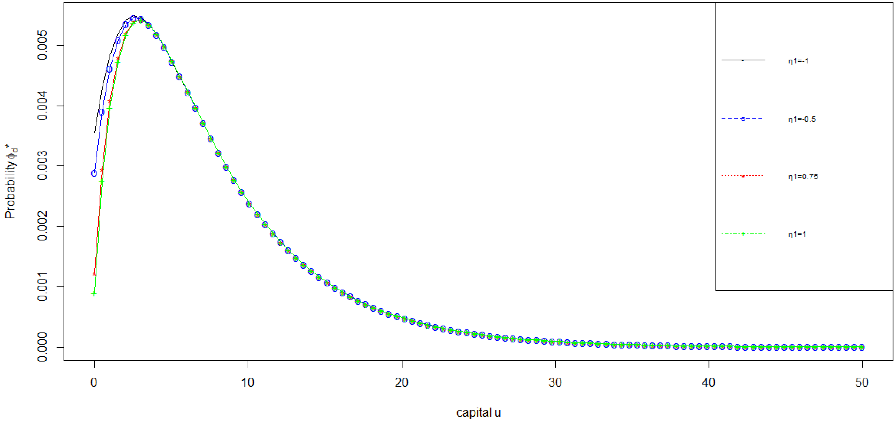
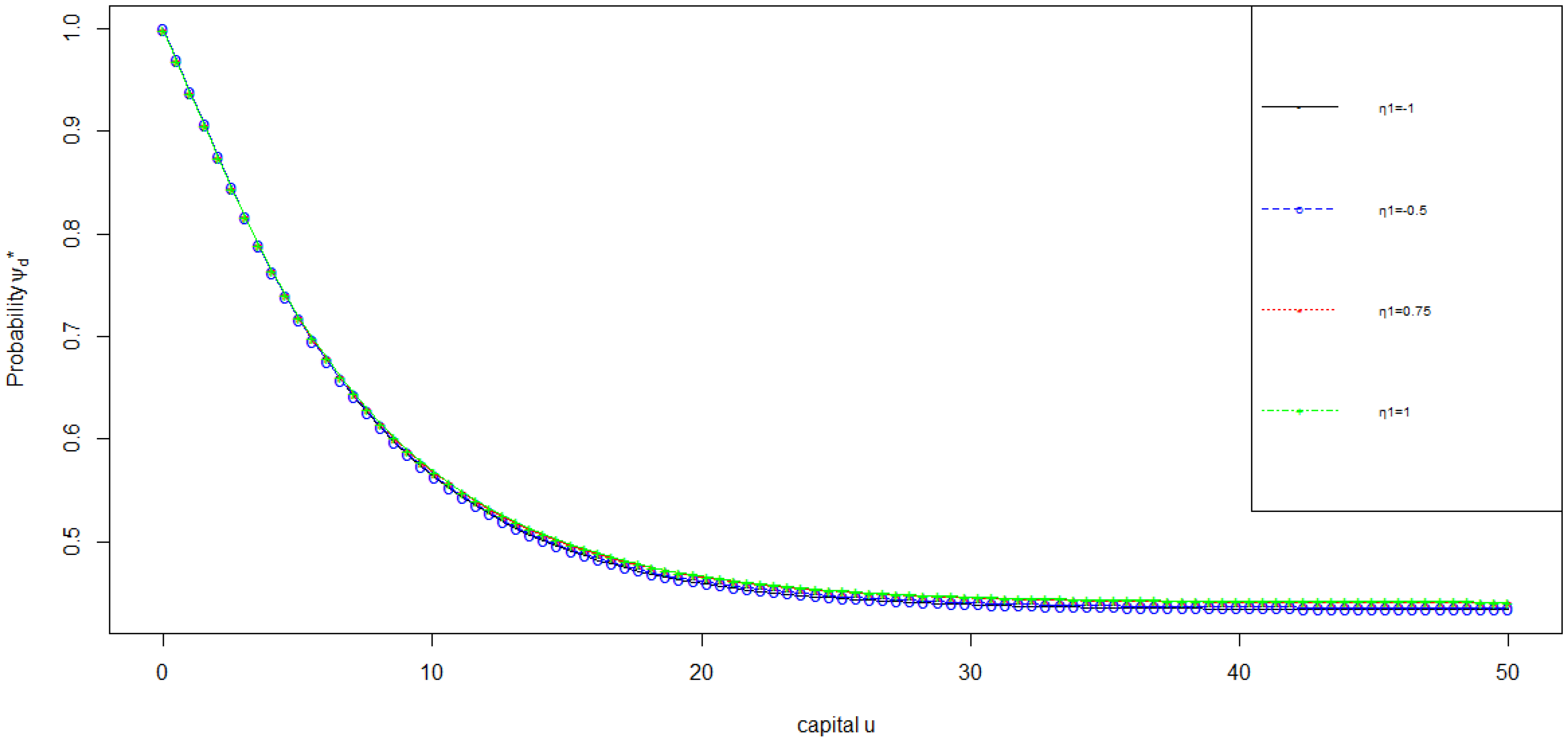
5. Numerical Illustration

In this section, we provide numerical examples of the Gerber–Shiu function where claims are exponentially distributed in the delayed and perturbed risk model of Type I, i.e., only the first claim is delayed from Theorem 7. Then, we provide numerical illustrations of the results from Theorem 8 of the risk model of Type II where the first two claims are delayed, with the first claim inter-occurrence’s time following a generalized mixed equilibrium distribution.
Table 1 provides the examples of the Gerber–Shiu functions of the first-order delayed and perturbed risk model (Type I). Figure 1 and Figure 2 illustrate the ruin probabilities of the second-order delayed and perturbed risk model (Type II) with λ 1 = 2 , θ 1 = 12.5 , q = 0.25 , δ = 0 , c = 2.5 , η 2 = 0.5 , θ 2 = 3.5 , θ = 2.75 , η = 0.5 , λ 2 = 1.85 , λ = 1.2 , σ = 5 and different values of η 1 . This implies for the first-order delayed and perturbed risk model (Type I) the following ruin probabilities:
ϕ d ( u ) = 0.0126 e 0.497 u 0.0104 e 0.653 u + 0.0129 e 0.163 u + 0.0177 e 0.556 u + 0.0004 e 2.768 u + 0.000013 e 5.509 u , ψ d ( u ) = 0.5441 e 0.497 u 0.261 e 0.653 u + 1.166 e 0.163 u + 0.631 e 0.556 u 0.0004 e 2.768 u 0.000013 e 5.509 u ,
and by the Theorem 8 we derive ϕ d and ψ d .
In Figure 1 and Figure 2 illustrating the ruin probabilities caused by claims and by oscillations of the second-order delayed and perturbed risk model (Type II), we notice that the ruin probabilities (caused by claims and by oscillations) both decrease as the initial capital increases.

6. Conclusions

We model insurance surplus by considering a second-order delayed and perturbed risk model and derived the Gerber–Shiu function. In this model, the occurrence time of the first claim follows a generalized mixed equilibrium distribution and the risk process becomes ordinary after the second claim. We derive the integro-differential equations of the Gerber–Shiu function when ruin is caused by claims and by oscillations. By considering exponential claim distribution, analytical expressions of the Gerber–Shiu functions are determined. The numerical illustration confirms the expectancy and the ruin probabilities (as special case of Gerber–Shiu function) caused by claims and oscillations both decrease as the initial capital is much more important.
Our main results are obtained from Equations (18) and (19) and can be further developed and extended in a few ways, which are the subject of future research. For example, one can try and obtain similar results to these two equations in some more general settings by first considering that the time occurrence of the first two claims and the inter-occurrence time of the subsequent claims follow Erlang(n) distributions with different parameters and second replacing the constant volatility by volatility that depends on the market mode or regime that switches among a finite number of states. Finally, one can also try to investigate in what ways the model can be extended so that it can be used to generalize the work of (Tan et al. 2020), who studied the optimal dynamic policy for an insurance company whose surplus is modelled by the diffusion approximation of the classical Cramer–Lundberg model.

Author Contributions

This doctoral research paper is done by E.T. under the supervision of F.A. All authors have read and agreed to the published version of the manuscript.

Funding

This work was supported by the Global Excellence and Stature (GES) 4.0 scholarship of the University of Johannesburg (UJ).

Acknowledgments

The authors would like to thank the anonymous referees for constructive comments that improved the contents and presentation of this paper.

Conflicts of Interest

The authors declare no conflict of interest.

References

  1. Borodin, Andrei N., and Paavo Salminen. 2002. Handbook of Brownian Motion-Facts and Formulae. Basel: Birkhäuser. [Google Scholar]
  2. Cai, Jun. 2007. On the time value of absolute ruin with debit interest. Advances in Applied Probability 39: 343–59. [Google Scholar] [CrossRef] [Green Version]
  3. Cai, Jun, Runhuan Feng, and Gordon E. Willmot. 2009. The compound poisson surplus model with interest and liquid reserves: Analysis of the gerber–shiu discounted penalty function. Methodology and Computing in Applied Probability 11: 401–23. [Google Scholar] [CrossRef]
  4. Chadjiconstantinidis, Stathis, and Spyridon Vrontos. 2014. On a renewal risk process with dependence under a farlie–gumbel–morgenstern copula. Scandinavian Actuarial Journal 2014: 125–58. [Google Scholar] [CrossRef] [Green Version]
  5. Cheung, Eric C. K., and Runhuan Feng. 2013. A unified analysis of claim costs up to ruin in a markovian arrival risk model. Insurance: Mathematics and Economics 53: 98–109. [Google Scholar] [CrossRef] [Green Version]
  6. Cheung, Eric C. K., David Landriault, Gordon E. Willmot, and Jae-Kyung Woo. 2010. Structural properties of gerber–shiu functions in dependent sparre andersen models. Insurance: Mathematics and Economics 46: 117–26. [Google Scholar] [CrossRef]
  7. Cossette, Héléne, Etienne Marceau, and Fouad Marri. 2010. Analysis of ruin measures for the classical compound poisson risk model with dependence. Scandinavian Actuarial Journal 2010: 221–45. [Google Scholar] [CrossRef]
  8. Dufresne, Francois, and Hans U. Gerber. 1991. Risk theory for the compound poisson process that is perturbed by diffusion. Insurance: Mathematics and Economics 10: 51–59. [Google Scholar] [CrossRef]
  9. Gao, Jianwei, and Liyuan Wu. 2014. On the gerber–shiu discounted penalty function in a risk model with two types of delayed-claims and random income. Journal of Computational and Applied Mathematics 269: 42–52. [Google Scholar] [CrossRef]
  10. Gerber, Hans U., and Bruno Landry. 1998. On the discounted penalty at ruin in a jump-diffusion and the perpetual put option. Insurance: Mathematics and Economics 22: 263–76. [Google Scholar] [CrossRef]
  11. Gerber, Hans U., and Elias S. W. Shiu. 1998. On the time value of ruin. North American Actuarial Journal 2: 48–72. [Google Scholar] [CrossRef]
  12. Kyprianou, Andreas E. 2006. Introductory Lectures on Fluctuations of Lévy Processes with Applications. Berlin: Springer Science & Business Media. [Google Scholar]
  13. Landriault, David, and Gordon Willmot. 2008. On the gerber–shiu discounted penalty function in the sparre andersen model with an arbitrary interclaim time distribution. Insurance: Mathematics and Economics 42: 600–8. [Google Scholar] [CrossRef]
  14. Lee, Wing Yan, and Gordon E. Willmot. 2014. On the moments of the time to ruin in dependent sparre andersen models with emphasis on coxian interclaim times. Insurance: Mathematics and Economics 59: 1–10. [Google Scholar] [CrossRef]
  15. Lin, X. Sheldon, and Gordon E. Willmot. 2000. The moments of the time of ruin, the surplus before ruin, and the deficit at ruin. Insurance: Mathematics and Economics 27: 19–44. [Google Scholar] [CrossRef]
  16. Nelsen, Roger B. 2006. An introduction to Copulas. Berlin: Springer Science & Business Media. [Google Scholar]
  17. Pavlova, Kristina P., and Gordon E. Willmot. 2004. The discrete stationary renewal risk model and the gerber–shiu discounted penalty function. Insurance: Mathematics and Economics 35: 267–77. [Google Scholar] [CrossRef]
  18. Schmidli, Hanspeter. 2010. On the gerber–shiu function and change of measure. Insurance: Mathematics and Economics 46: 3–11. [Google Scholar] [CrossRef]
  19. Schmidli, Hanspeter. 2014. A note on gerber–shiu functions with an application. In Modern Problems in Insurance Mathematics. Cham: Springer, pp. 21–36. [Google Scholar]
  20. Tan, Ken Seng, Pengyu Wei, Wei Wei, and Sheng Chao Zhuang. 2020. Optimal dynamic reinsurance policies under a generalized denneberg’s absolute deviation principle. European Journal of Operational Research 282: 345–62. [Google Scholar] [CrossRef]
  21. Tsai, Cary Chi-Liang, and Gordon E. Willmot. 2002. A generalized defective renewal equation for the surplus process perturbed by diffusion. Insurance: Mathematics and Economics 30: 51–66. [Google Scholar] [CrossRef] [Green Version]
  22. Wang, Guojing. 2001. A decomposition of the ruin probability for the risk process perturbed by diffusion. Insurance: Mathematics and Economics 28: 49–59. [Google Scholar] [CrossRef]
  23. Willmot, Gordon E. 2004. A note on a class of delayed renewal risk processes. Insurance: Mathematics and Economics 34: 251–57. [Google Scholar] [CrossRef]
  24. Willmot, Gordon E. 2007. On the discounted penalty function in the renewal risk model with general interclaim times. Insurance: Mathematics and Economics 41: 17–31. [Google Scholar] [CrossRef]
  25. Willmot, Gordon E., and David C. M. Dickson. 2003. The gerber–shiu discounted penalty function in the stationary renewal risk model. Insurance: Mathematics and Economics 32: 403–11. [Google Scholar] [CrossRef] [Green Version]
  26. Willmot, Gordon E., X. Sheldon Lin, and X. Sheldon Lin. 2001. Lundberg Approximations for Compound Distributions with Insurance Applications. Berlin: Springer Science & Business Media, vol. 156. [Google Scholar]
  27. Zhang, Zhimin, and Hu Yang. 2011. Gerber–shiu analysis in a perturbed risk model with dependence between claim sizes and interclaim times. Journal of Computational and Applied Mathematics 235: 1189–204. [Google Scholar] [CrossRef]
  28. Zhang, Zhimin, Shuanming Li, and Hu Yang. 2009. The gerber–shiu discounted penalty functions for a risk model with two classes of claims. Journal of Computational and Applied Mathematics 230: 643–55. [Google Scholar] [CrossRef] [Green Version]
  29. Zhou, Ming, and Jun Cai. 2009. A perturbed risk model with dependence between premium rates and claim sizes. Insurance: Mathematics and Economics 45: 382–92. [Google Scholar] [CrossRef]
  30. Zou, Wei, and Jie-hua Xie. 2012. On the gerber–shiu discounted penalty function in a risk model with delayed claims. Journal of the Korean Statistical Society 41: 387–97. [Google Scholar] [CrossRef]
Figure 1. Ruin probabilities caused by claims: ϕ d .
Risks 08 00030 g001
Figure 2. Ruin probabilities caused by oscillation: ψ d .
Risks 08 00030 g002
Table 1. Numerical illustration when claims are exponentially distributed under the risk model of Type I.
δ = 0 , c = 2.5 , η 2 = 0.5 , θ 2 = 3.5 , θ = 2 , η = 0.5 , λ 2 = 1.85 , λ = 1.2 , σ = 5
ϕ d ( u ) = 0.00133 e 0.4975 u 0.01027 e 0.6532 u + 0.00805 e 0.1713 u + 0.0113 e 0.5544 u + 0.0063 e 3.5142 u 0.00157 e 7.0071 u
ψ d ( u ) = 0.6178 e 0.4975 u 0.2604 e 0.6532 u + 1.1885 e 0.1713 u + 0.6817 e 0.5544 u + 0.0063 e 3.5142 u + 0.0016 e 7.0071 u
δ = 0 , c = 4.25 , η 2 = 0.75 , θ 2 = 1.75 , θ = 2.75 , η = 0.5 , λ 2 = 1.75 , λ = 1.25 , σ = 3.5
ϕ d ( u ) = 0.8794 e 0.9842 u 3.6173 e 1.1786 u + 0.04781 e 0.602 u + 0.471 e 1.096 u 0.00576 e 2.794 u 0.00003 e 5.5216 u
ψ d ( u ) = 15.692 e 0.9842 u 26.884 e 1.1786 u + 2.772 e 0.602 u + 34.276 e 1.096 u + 0.00565 e 2.794 u + 0.000031 e 5.5216 u
δ = 0.15 , c = 7.25 , η 2 = 0.75 , θ 2 = 1.25 , θ = 2.75 , η = 0.65 , λ 2 = 4.75 , λ = 2.25 , σ = 1.5
ϕ d ( u ) = 0.30002 e 7.0613 u + 1.79386 e 7.5766 u 0.8468 e 2.4623 u 0.0012 e 5.0643 u + 0.01598 e 6.6421 u 1.9103 e 7.5663 u
ψ d ( u ) = 9.248 e 7.0613 u + 42.547 e 7.5766 u 1.046 e 2.4623 u 0.02024 e 5.0643 u 1.0286 e 6.6421 u 49.8108 e 7.5663 u

