A Survey of the Individual Claim Size and Other Risk Factors Using Credibility Bonus-Malus Premiums

Abstract

In this paper, a flexible count regression model based on a bivariate compound Poisson distribution is introduced in order to distinguish between different types of claims according to the claim size. Furthermore, it allows us to analyse the factors that affect the number of claims above and below a given claim size threshold in an automobile insurance portfolio. Relevant properties of this model are given. Next, a mixed regression model is derived to compute credibility bonus-malus premiums based on the individual claim size and other risk factors such as gender, type of vehicle, driving area, or age of the vehicle. Results are illustrated by using a well-known automobile insurance portfolio dataset.

1. Introduction

In a recent work, a modification in the bonus-malus systems was proposed Gómez-Déniz (2016), which are commonly applied in automobile insurance, that differentiated between two different types of claims by including a bivariate model based on the assumption of dependence. The aforementioned work studied the impact on the bonus-malus premium in a general setting without involving individual’s risk factors, such as gender, type of vehicle, area of circulation, etc.

It is well known that under the traditional bonus-malus system, the premium charged to each insured is based solely on the number of claims made. Therefore, an insured who has had an accident that causes a relatively small loss amount is penalised to the same extent as one who has experienced a more expensive accident. This event would seem to be unfair by the insureds. In the mentioned work a bivariate prior model, conjugated with respect to the likelihood, was also proposed, and as a result of this, simple credibility bonus-malus premiums that satisfy appropriate transition rules were obtained. These expressions were used to compute credibility bonus-malus premiums by considering two different types of claims: those ones above and below a threshold claim size, say $\psi >0$.

Similar related works have been proposed in the actuarial literature. In this sense, the work in Pinquet (1998) computed bonus-malus rates in a multi-equation Poisson model with random effects. The work in Ragulina (2011) introduced a bonus-malus system with different claim types and varying deductibles. The work in Walhin and Paris (2001) showed how to set up a practical bonus-malus system with a finite number of classes using both the actual claim amount and claim frequency distribution. The work in Bonsdorff (2005) also incorporated the claim number and the severity in the bonus-malus system literature by using Markov chains. The work in Bermúdez (2009) examined, in automobile insurance claims, an a priori ratemaking procedure that included two different types of claim, i.e., with and without bodily injuries. See also Bermúdez and Karlis (2017).

The main objective of this work is to develop a reparametrization of the bivariate distribution proposed in the previous work with the purpose of incorporating individual information in the model to adjust the premiums charged to each policyholder. Additionally, some statistical properties of the proposed parametrization that were not addressed in the previous work will be shown. Furthermore, an extensive set of a priori classification variables such as age, gender, type and age of car, etc., will be used to incorporate, depending on the heterogeneity of the insured’s behaviour, prior distributions assigned to the parameters of the model to build up a posteriori credibility, bonus-malus premiums.

The rest of this paper is organised as follows. The main model and some of its properties are presented in Section 2. In Section 3, the regression model is introduced, and maximum likelihood estimation methods are illustrated. We will show that the estimation procedure is simply derived, and Fisher’s information matrix associated with this regression model is obtained in closed-form. Credibility premiums related to the regression models are provided in Section 4. Numerical illustrations and results connected with the compound model are shown in Section 5, and finally, Section 6 concludes the work.

2. The Model

As pointed out by Dionne and Vanasse (1989), the classical Poisson distribution is generally employed for the characterization of random and independent events such as automobile accidents. Thus, we assume that the number of claims in an automobile insurance portfolio follows a Poisson distribution with parameter ${\mu }_1>0$. When an insured declares a claim, it might be for an amount exceeding $\psi$ monetary units. In order to accommodate this characteristic into the model, we incorporate a second random variable, thus giving rise to the consideration of two separate sub-events (claims worth more or less than $\psi$), in the following way. Let $Z_i$ be the variable that takes the value one if the $i^{\mathrm{th}}$ claim corresponds to a claim size larger than $\psi$ and the value zero otherwise. Thus, the $Z_i^{\prime }s$ variables are modelled as independent and identically distributed with the following Bernoulli probability density function:

$$f\left(z_i\right|p)=\left\{\begin{array}{ccc}{\mu }_2/{\mu }_1,\hfill & if& \hfill z_i=1,\\ 1-{\mu }_2/{\mu }_1,\hfill & if& \hfill z_i=0,\end{array}\right.$$

where $p={\mu }_2/{\mu }_1$ is the probability of declaring a claim larger than $\psi$ with $0<{\mu }_2<{\mu }_1$.

Let us now assume that $X_2={\sum }_{i=1}^{X_1}{Z}_i$ is the total claim number with a claim amount larger than $\psi$. Thus, if the $Z_i$$(i=1,\cdots ,x_1)$ are assumed to be mutually independent, then the conditional probability function of $X_2$, given that $X_1=x_1$, is binomial with parameters $x_1$ and ${\mu }_2/{\mu }_1$. Therefore, the joint distribution of the total claim number ($X_1$) and the corresponding claim number with claim amount exceeding $\psi$, $X_2$, has this probability function:

$$\begin{array}{c}\hfill Pr(X_1=x_1,X_2=x_2)=\frac{{\mu }_2^{x_2}{({\mu }_1-{\mu }_2)}^{x_1-x_2}exp(-{\mu }_1)}{(x_1-x_2)!x_2!},\end{array}$$

(1)

for $x_1=0,1,\cdots ,$$x_2=0,1,\cdots ,x_1$, ${\mu }_1>0$, and $0<{\mu }_2<{\mu }_1$.

Observe that the probability function (1) can be written as:

$$\begin{array}{c}\hfill Pr(X_1=x_1,X_2=x_2)=h\left(\mathit{x}\right)exp\left[\sum _{i=1}^2{x}_i{R}_i\left(\mathsf{\Theta }\right)-Q\left(\mathsf{\Theta }\right)\right],\end{array}$$

where $\mathit{x}=(x_1,x_2)$, $\mathsf{\Theta }={({\mu }_1,{\mu }_2)}^{\prime }$, $R_1\left(\mathsf{\Theta }\right)=log({\mu }_1-{\mu }_2)$, $R_2\left(\mathsf{\Theta }\right)=log({\mu }_2/({\mu }_1-{\mu }_2))$, $Q\left(\mathsf{\Theta }\right)={\mu }_1$, and $h\left(\mathit{x}\right)={[(x_1-x_2)!x_2!]}^{-1}$. Thus, (1) belongs to the multivariate exponential family of distributions provided in Khatri (1983a). See also Khatri (1983b) and Johnson et al. (1997, chp. 34). This family includes also the multivariate Lagrangian distributions and the multivariate power series distributions; (see Khatri 1983b).

Properties of the Distribution

The marginal means are given by $E\left(X_i\right)={\mu }_i$, $i=1,2$. The cross moment, the covariance, and the correlation are given by:

$$\begin{array}{ccc}\hfill E\left(X_1{X}_2\right|{\mu }_1,{\mu }_2)& =& {\mu }_2(1+{\mu }_1),\hfill \\ \hfill cov(X_1,X_2|{\mu }_1,{\mu }_2)& =& {\mu }_2,\hfill \\ \hfill \rho (X_1,X_2|{\mu }_1,{\mu }_2)& =& \sqrt{{\mu }_2/{\mu }_1},\hfill \end{array}$$

(2)

respectively. Thus, the model admits only positive correlation.

The probabilities for different values of $(x_1,x_2)$ were calculated, and  graphs were plotted for different values of these two parameters. They are shown in Figure 1. It is observable that for larger values of ${\mu }_1$ and ${\mu }_2$, the modal value increases in $x_1$ and $x_2$, illustrating that the new model is very  versatile.

The expression provided in (1) can also be obtained differently as follows: Let us consider an automobile insurance portfolio in which $X_1$ is a random variable that represents the number of claims in a given period and $X_2$ yields the number of claims with a size above a threshold $\psi >0$ over the same period of time. If  each policyholder has a probability ${\mu }_2/{\mu }_1$ of having a claim with a claim size above $\psi$, then $Pr(X_2=x_2)$ and $Pr(X_1=x_1)$ are related as follows:

$$\begin{array}{c}\hfill Pr(X_2=x_2)=\sum _{x_1=x_2}^{\infty }\left(\genfrac{}{}{0pt}{}{x_1}{x_2}\right){\left(\frac{{\mu }_2}{{\mu }_1}\right)}^{x_2}{\left(1-\frac{{\mu }_2}{{\mu }_1}\right)}^{x_1-x_2}Pr(X_1=x_1).\end{array}$$

(3)

Obviously, (3) represents a map from the probability function to the probability function. That is, ${\sum }_{x_2=0}^{\infty }Pr(X_2=x_2)=1$ with $Pr(X_2=x_2)\ge 0$, $x_2=0,1,\cdots$

Although other distributions, i.e., negative binomial, could be chosen to model count data, for the sake of simplicity, let us suppose that $X_1$ follows a Poisson distribution with parameter ${\mu }_1>0$. Then, we have:

$$\begin{array}{ccc}\hfill Pr(X_2=x_2)& =& \sum _{x_1=x_2}^{\infty }\left(\genfrac{}{}{0pt}{}{x_1}{x_2}\right){\left(\frac{{\mu }_2}{{\mu }_1}\right)}^{x_2}{\left(1-\frac{{\mu }_2}{{\mu }_1}\right)}^{x_1-x_2}\frac{{\mu }_1^{x_1}exp(-{\mu }_1)}{x_1!}\hfill \\ & =& \frac{exp(-{\mu }_1)}{x_2!}{\left(\frac{{\mu }_2}{{\mu }_1-{\mu }_2}\right)}^{x_2}\sum _{x_1=x_2}^{\infty }\frac{{({\mu }_1-{\mu }_2)}^{x_1}}{(x_1-x_2)!}\hfill \\ & =& \frac{{\mu }_2^{x_2}exp(-{\mu }_1)}{x_2!}\sum _{j=0}^{\infty }\frac{{({\mu }_1-{\mu }_2)}^j}{j!}\hfill \\ & =& \frac{{\mu }_2^{x_2}}{x_2!}exp(-{\mu }_2),x_2=0,1,\cdots \hfill \end{array}$$

Expression (3) can be viewed as a weighted sum of binomial probabilities where the weights are given by the probability that the policyholder declares a certain number of claims. More specifically, it is the mean of the total number of claims with a threshold conditional on the fact that $X_1=x_1$ claims and assuming the existence of a heterogeneity factor that causes different claims of different amounts. Hence, Expression (3) can be viewed as a mixture distribution. From this standpoint, the model provides a framework in which random effects are incorporated into the Poisson assumption. In this case, the bivariate distribution provided in (1) can be obtained by multiplying the conditional and the marginal distributions in the usual way.

Numerical simulation of the bivariate distribution can be simply obtained by following the approach explained in Kocherlakota and Kocherlakota (1992, chp. 1). In this regard, both the marginal distribution $f\left(x_1\right)$ and the conditional distribution $f\left(x_2\right|x_1)$ will be used. The former is a Poisson distribution with parameter ${\mu }_1$ and the latter a binomial distribution with parameters x and ${\mu }_2/{\mu }_1$. Thus, for specific values of $x_1$, a realization of $x_2$ from $f\left(x_2\right|x_1)$ can be generated, and therefore, the pairs $(x_1,x_2)$ are observations from the joint distribution given in (1). This procedure can be repeated n times in order to obtain a random sample of size n.

The joint probability generating function is given by:

$$\begin{array}{c}\hfill G_{X_1,X_2}(s_1,s_2)=exp[{\mu }_1(s_1-1)+{\mu }_2(s_2-1)s_1],|s_1|\le 1,|s_2|\le 1.\end{array}$$

(4)

Note that (4) is the limiting case of the bivariate Poisson distribution with parameters ${\theta }_1={\mu }_1-{\mu }_2$, ${\theta }_2\to 0$, and ${\theta }_{12}={\mu }_2$ (see for instance this expression in (Johnson et al. 1997, chp. 37) and also Hesselager (1996) for more details of recursions for bivariate discrete distributions). Thus, the following recursions are valid:

$$\begin{array}{ccc}\hfill p_{x_1,x_2}& =& \frac{{\mu }_1-{\mu }_2}{x_1}{p}_{x_1-1,x_2}+\frac{{\mu }_2}{x_1}{p}_{x_1-1,x_2-1},\hfill \\ \hfill p_{x_1,x_2}& =& \frac{{\mu }_2}{x_2}{p}_{x_1-1,x_2-1},\hfill \end{array}$$

with:

$$\begin{array}{ccc}\hfill p_{0,0}& =& exp(-{\mu }_1),\hfill \\ \hfill p_{x_1,0}& =& \frac{{({\mu }_1-{\mu }_2)}^{x_1}exp(-{\mu }_1)}{x_1!},\hfill \end{array}$$

and zero otherwise.

3. The Role of the Covariates

Clearly, the number of claims below and above $\psi$ may be influenced by different characteristics and factors; likewise, explanatory variables may be useful to explain the individual premium to be charged. As (1) satisfies that the marginal means are given by $E\left(X_1\right)={\mu }_1$ and $E\left(X_2\right)={\mu }_2$, then covariates can be simply implemented in the model.

We now investigate the effect of including covariates to account for the total number of claims and the claims above the threshold $\psi$. Obviously, some factors are crucial when explaining the endogenous variables $(X_{1i},X_{2i})$. Two appropriate links are needed to connect the explanatory variables with the marginal means. A natural way to proceed is to assume that $(X_{1i},X_{2i})$ for $i=1,\cdots ,n$ follows the probability function (1) and:

$$\begin{array}{ccc}\hfill log{\mu }_{1i}& =& {\omega }_{1i}{\beta }_1,\hfill \\ \hfill {\mu }_{2i}& =& \frac{{\mu }_{1i}exp\left({\eta }_{2i}{\beta }_2\right)}{1+exp\left({\eta }_{2i}{\beta }_2\right)},\hfill \end{array}$$

where ${\omega }_{1i}$ and ${\eta }_{2i}$ denote vectors of m explanatory variables for the $i^{\mathrm{th}}$ observation, i.e., with components ${\omega }_{ji}$ and ${\eta }_{ji}$, $(j=1,\cdots ,m)$, used to model ${\mu }_{1i}$ and ${\mu }_{2i}$, respectively, and where ${\beta }_k={({\beta }_{k1},\cdots ,{\beta }_{km})}^{\top }$, $(k=1,2)$ designates the corresponding vector of regression coefficients. The log-linear specification for ${\mu }_{1i}$ is widely used, while the link function for ${\mu }_{2i}$ was chosen in this way to ensure that the latter one would not be larger than ${\mu }_{1i}$, and thus, it would be compatible with $X_2\le X_1$.

These mean values may be influenced by several characteristics and variables, and the explanatory variables that are used to model each parameter ${\mu }_{1i}$ and ${\mu }_{2i}$ may not be the same in practice. In this respect, the work in Cameron and Trivedi (1998) provided good insight into standard count regression models.

The marginal effect reflects the variation of the conditional mean of $X_1$ and $X_2$ due to a one-unit change in the $j^{\mathrm{th}}$ covariate, and it is calculated as:

$$\begin{array}{ccc}\hfill \frac{\partial {\mu }_{1i}}{\partial {\beta }_{1j}}& =& {\omega }_{ji}exp\left({\omega }_{1i}{\beta }_1\right)={\omega }_{ji}{\mu }_{1i},\hfill \\ \hfill \frac{\partial {\mu }_{2i}}{\partial {\beta }_{2j}}& =& {\eta }_{ji}{\mu }_{2i}\left(1-\frac{{\mu }_{2i}}{{\mu }_{1i}}\right),\hfill \end{array}$$

(5)

for $i=1,\cdots ,n$ and $j=1,\cdots ,m$. Thus, the marginal effect indicates that a one-unit change in the $j^{\mathrm{th}}$ regressor increases or decreases the expectation of the total number of claims and the number of claims above the given threshold depending on the sign, positive or negative, of the regressor for each mean. For indicator variables such as ${\omega }_{ik}$, which takes only the value zero or one, the marginal effect in terms of the odds-ratio is $exp\left({\beta }_{1j}\right)$ for ${\mu }_{i1}$ and $exp\left({\beta }_{2j}\right)$ for ${\mu }_{i2}$. Therefore, for ${\mu }_{i1}$, the  conditional mean is $exp\left({\beta }_{1j}\right)$ times larger if the indicator is one rather than zero. A similar conclusion is drawn for ${\mu }_{i2}$. Certainly, if ${\mu }_{1i}$ and ${\mu }_{2i}$ share the same covariates, then (5) does not correspond to the marginal effect of the $j^{\mathrm{th}}$ covariate since ${\mu }_{1i}$ may also change in response to the changes of this covariate.

3.1. Estimation

In this section, we derive estimators based on the maximum likelihood for the model with and without covariates, and we also provide closed-form expressions for Fisher’s information matrix.

3.1.1. Model without Covariates

Let $\mathsf{\Theta }=({\mu }_1,{\mu }_2)$ and a random sample consisting of n observations $\mathit{x}=\{(x_{11},x_{21}),\cdots ,(x_{1n},x_{2n})\}$, taken from the probability function (1). The log-likelihood is proportional to:

$$\begin{array}{c}\hfill \ell (\mathsf{\Theta };\mathit{x})\propto n{\overline{x}}_{2}log{\mu }_2+n({\overline{x}}_1-{\overline{x}}_2)log({\mu }_1-{\mu }_2)-n{\mu }_1,\end{array}$$

where ${\overline{x}}_1$ and ${\overline{x}}_2$ are the sample means of $X_1$ and $X_2$, respectively. The normal equations to be solved are:

$$\begin{array}{ccc}\hfill \frac{\partial \ell (\mathsf{\Theta };\mathit{x})}{\partial {\mu }_1}& =& \frac{n({\overline{x}}_1-{\overline{x}}_2)}{{\mu }_1-{\mu }_2}-n=0,\hfill \\ \hfill \frac{\partial \ell (\mathsf{\Theta };\mathit{x})}{\partial {\mu }_2}& =& \frac{n{\overline{x}}_2}{{\mu }_2}+\frac{n({\overline{x}}_2-{\overline{x}}_1)}{{\mu }_1-{\mu }_2}=0,\hfill \end{array}$$

from which it is easy to obtain the solution to obtain the maximum likelihood estimators ${\widehat{\mu }}_1={\overline{x}}_1$ and ${\widehat{\mu }}_2={\overline{x}}_2$ which coincide with the moment estimators. The second partial derivatives are:

$$\begin{array}{ccc}\hfill \frac{{\partial }^2\ell (\mathsf{\Theta };\mathit{x})}{\partial {\mu }_1^2}& =& -\frac{n({\overline{x}}_1-{\overline{x}}_2)}{{({\mu }_1-{\mu }_2)}^2},\hfill \\ \hfill \frac{{\partial }^2\ell (\mathsf{\Theta };\mathit{x})}{\partial {\mu }_2^2}& =& -\frac{n{\overline{x}}_2}{{\mu }_2^2}+\frac{n({\overline{x}}_2-\overline{x})}{{({\mu }_1-{\mu }_2)}^2},\hfill \\ \hfill \frac{{\partial }^2\ell (\mathsf{\Theta };\mathit{x})}{\partial {\mu }_1\partial {\mu }_2}& =& \frac{n({\overline{x}}_1-{\overline{x}}_2)}{{({\mu }_1-{\mu }_2)}^2}.\hfill \end{array}$$

The expectation of the negative of the second partial derivative yields Fisher’s information matrix:

$$\mathcal{J}\left(\widehat{\mathsf{\Theta }}\right)=\left[\begin{array}{cc}\frac{n}{{\widehat{\mu }}_1-{\widehat{\mu }}_2}& \frac{n{\widehat{\mu }}_1}{{\widehat{\mu }}_2({\widehat{\mu }}_1-{\widehat{\mu }}_2)}\\ \frac{n{\widehat{\mu }}_1}{{\widehat{\mu }}_2({\widehat{\mu }}_1-{\widehat{\mu }}_2)}& \frac{n}{{\widehat{\mu }}_2-{\widehat{\mu }}_1}\end{array}\right].$$

The asymptotic variance-covariance matrix of $({\widehat{\mu }}_1,{\widehat{\mu }}_2)$ is obtained by inverting this information matrix.

3.1.2. Model with Covariates

When covariates are considered, the log-likelihood is proportional to:

$$\begin{array}{c}\hfill \ell (\mathit{\beta };\mathit{x})\propto \sum _{i=1}^n\left[x_{2i}log{\mu }_{2i}+(x_{1i}-x_{2i})log({\mu }_{1i}-{\mu }_{2i})-{\mu }_{1i}\right],\end{array}$$

(6)

where $\mathit{\beta }=({\beta }_1,{\beta }_2)$.

Observe now that ${\mu }_{1i}={\mu }_{1i}\left({\beta }_1\right)$ and ${\mu }_{2i}={\mu }_{2i}({\beta }_1,{\beta }_2)$, to emphasize that the first expression depends only on ${\beta }_1$ and the second on both ${\beta }_1$ and ${\beta }_2$. Thus,

$$\begin{array}{c}\hfill \frac{\partial {\mu }_{1i}}{\partial {\beta }_{1j}}={\omega }_{ji}{\mu }_{1i},\frac{\partial {\mu }_{2i}}{\partial {\beta }_{1j}}={\omega }_{ji}{\mu }_{2i},\frac{\partial {\mu }_{2i}}{\partial {\beta }_{2j}}=\frac{{\mu }_{2i}{\eta }_{ji}}{1+exp\left({\eta }_{2i}\right)},\end{array}$$

for $i=1,\cdots ,n$ and $j=1,\cdots ,m$.

Then, after some algebra, we obtain the normal equations,

$$\begin{array}{ccc}\hfill \frac{\partial \ell (\mathit{\beta };\mathit{x})}{\partial {\beta }_{1j}}& =& \sum _{i=1}^n{\omega }_{ji}(x_{1i}-{\mu }_{1i})=0,j=1,\cdots ,m,\hfill \\ \hfill \frac{\partial \ell (\mathit{\beta };\mathit{x})}{\partial {\beta }_{2j}}& =& \sum _{i=1}^n\frac{{\eta }_{ji}\varphi ({\mu }_{1i},{\mu }_{2i},x_{1i},x_{2i})}{1+exp\left({\eta }_{2i}{\beta }_2\right)}=0,j=1,\cdots ,m,\hfill \end{array}$$

where:

$$\begin{array}{c}\hfill \varphi ({\mu }_{1i},{\mu }_{2i},x_{1i},x_{2i})=\frac{x_{2i}{\mu }_{1i}-x_{1i}{\mu }_{2i}}{{\mu }_{1i}-{\mu }_{2i}}.\end{array}$$

These equations provide the maximum likelihood estimates for the vector of parameters ${\widehat{\beta }}_1={({\widehat{\beta }}_{11},\cdots ,{\widehat{\beta }}_{1m})}^{\top }$ and ${\widehat{\beta }}_2={({\widehat{\beta }}_{21},\cdots ,{\widehat{\beta }}_{2m})}^{\top }$. Similarly to the previous case, Fisher’s information matrix can be obtained in closed-form. See the details in Appendix A.

The normal equations illustrated above can be used to estimate model parameters with and without covariates. The Newton–Raphson method provides solutions in a non-prohibitive time, obviously depending on the number of regressors used.

4. Credibility Regression Premiums

Briefly speaking, a bonus-malus system is an experience rating system that is based on the insured’s claim experience frequency rather than the claim size. Let us now assume some kind of heterogeneity between policyholders, by allowing that the parameters ${\mu }_i$, $i=1,2$ follow some probability functions. For ${\mu }_1$, a gamma prior distribution will be assumed ${\pi }_1\left({\mu }_1\right)$ with a shape hyperparameter ${\alpha }_1>0$ and a scale hyperparameter ${\gamma }_1>0$, whereas a type beta prior distribution will be considered for ${\mu }_2$ with the probability density function given by:

$$\begin{array}{c}\hfill {\pi }_2\left({\mu }_2\right)=\frac{{\mu }_2^{{\alpha }_2-1}{({\mu }_1-{\mu }_2)}^{{\gamma }_2-1}}{{\mu }_1^{{\alpha }_2+{\gamma }_2-1}B({\alpha }_2,{\gamma }_2)},0<{\mu }_2<{\mu }_1.\end{array}$$

Here, ${\alpha }_2>0$, ${\gamma }_2>0$, and $B(a,b)$ is the beta function given by $B(a,b)=\mathsf{\Gamma }\left(a\right)\mathsf{\Gamma }\left(b\right)/\mathsf{\Gamma }(a+b)$ where $\mathsf{\Gamma }(·)$ is the Euler gamma function.

The main benefit of selecting these prior distributions is that they are conjugate with respect to the likelihoods, and for that reason, they are common choices in Bayesian and actuarial statistics; see for instance Heilmann (1989); Denuit et al. (2009), and Klugman et al. (2008), among others.

Since ${\mu }_1$ and ${\mu }_2$ are dependent, we can choose the prior distribution given by:

$$\begin{array}{c}\hfill \pi ({\mu }_1,{\mu }_2)={\pi }_1\left({\mu }_1\right){\pi }_2\left({\mu }_2\right)[1+\omega {\varphi }_1\left({\mu }_1\right){\varphi }_2\left({\mu }_2\right)],\end{array}$$

(7)

which corresponds to the copula proposed by Lee (1996). Here, ${\varphi }_i\left({\mu }_i\right)$, $i=1,2$, are bounded non-constant functions such that $\int {\pi }_i\left({\mu }_i\right){\varphi }_i\left({\mu }_i\right)d{\mu }_i=0$, and $\omega$ a real number, which satisfies that $1+\omega {\varphi }_i\left({\mu }_i\right)\ge 0$, $i=1,2$. Now, given a sample $\mathit{x}=({\tilde{x}}_1,{\tilde{x}}_2)=\{(x_{11},x_{21}),\cdots ,(x_{1t},x_{2t})\}$, where t is the sample size, the posterior distribution of $({\mu }_1,{\mu }_2)$ given the sample information is computed according to Bayes’ theorem, and it is proportional to the product of the likelihood and the prior distribution. Thus, the posterior distribution is almost conjugated with respect to the likelihood and similar to the product of a gamma and a beta distribution and where the updated parameters are given by:

$$\begin{array}{ccc}\hfill {\alpha }_1^{*}& =& {\alpha }_1+t{\overline{x}}_1,\hfill \end{array}$$

(8)

$$\begin{array}{ccc}\hfill {\alpha }_2^{*}& =& {\alpha }_2+t{\overline{x}}_2,\hfill \end{array}$$

(9)

$$\begin{array}{ccc}\hfill {\gamma }_1^{*}& =& {\gamma }_1+t,\hfill \end{array}$$

(10)

$$\begin{array}{ccc}\hfill {\gamma }_2^{*}& =& {\gamma }_2+t({\overline{x}}_1-{\overline{x}}_2).\hfill \end{array}$$

(11)

In practise, it is shown that ${\mu }_2$ is near zero, then in this case, $\omega \to 0$, and the prior distribution reduces to $\pi ({\mu }_1,{\mu }_2)={\pi }_1\left({\mu }_1\right){\pi }_2\left({\mu }_2\right)$, which is the case considered here.

Now, the unconditional means and cross moment are given by:

$$\begin{array}{ccc}\hfill E\left(X_1\right)& =& \frac{{\alpha }_1}{{\gamma }_1},\hfill \\ \hfill E\left(X_2\right)& =& \frac{{\alpha }_1}{{\gamma }_1}\frac{{\alpha }_2}{{\alpha }_2+{\gamma }_2},\hfill \\ \hfill E\left(X_1{X}_2\right)& =& \frac{{\alpha }_1{\alpha }_2({\alpha }_1+{\gamma }_1+1)}{{\gamma }_1^2({\alpha }_2+{\gamma }_2)}.\hfill \end{array}$$

Finally, the unconditional bivariate distribution is:

$$\begin{array}{ccc}\hfill Pr(X_1=x_1,X_2=x_2)& =& \frac{{\gamma }_1^{{\alpha }_1}}{{(1+{\gamma }_1)}^{x_1+{\alpha }_1}}\hfill \\ & & \times \frac{\mathsf{\Gamma }(x_1+{\alpha }_1)\mathsf{\Gamma }(x_2+{\alpha }_2)\mathsf{\Gamma }(x_1-x_2+{\gamma }_2)}{(x_1-x_2)!x_2!B({\alpha }_2,{\gamma }_2)\mathsf{\Gamma }\left({\alpha }_1\right)\mathsf{\Gamma }({\alpha }_2+{\gamma }_2+x_1)}.\hfill \end{array}$$

(12)

For computational reasons, sometimes, it is more convenient to work with the parametrization ${\alpha }_1={\gamma }_1{\mu }_1$ and ${\alpha }_2={\gamma }_2{\mu }_2/({\mu }_1-{\mu }_2)$.

The maximum likelihood estimates for this mixture regression model can be simply obtained by means of the EM algorithm. This method is a powerful technique that provides an iterative procedure to compute maximum likelihood estimation when data contain missing information. Details on the derivation of the EM algorithm can be found in Appendix B. The standard errors of the estimates $\widehat{\mathsf{\Omega }}=({\widehat{\beta }}_1,{\widehat{\beta }}_2,{\widehat{\gamma }}_1,{\widehat{\gamma }}_2)$ can be computed by using the method given by Louis (1982). Here, we use Fisher’s information matrix found in Appendix A and replace the missing values by the corresponding pseudo-values calculated in the last iteration of the EM algorithm. Direct maximization of the likelihood surface is also possible to compute the maximum likelihood estimates of the mixture regression model.

By following the same arguments as those ones provided in Gómez-Déniz (2016) and also based on the ideas in Heilmann (1989) (see also Gerber 1979, Rolski et al. 1999, Bühlmann and Gisler 2005, and Gómez-Déniz 2008; among others), a premium calculation principle assigns to each risk vector of parameters $\mathsf{\Theta }$ a premium within the set $P\in \mathbb{R}$, the action space. Let $L(\mathsf{\Theta },P)={(\mathsf{\Theta }-P)}^2$ be the squared-error loss function sustained by a decision-maker who takes the action P and is faced with the outcome $\mathsf{\Theta }$ of a random experience. The premium must be determined in a way such that the expected loss is minimised. The unknown premium $P\left(\mathsf{\Theta }\right)$, called the risk premium, can be obtained by minimising ${(g(x_1,x_2)-P)}^2$, where $g(x_1,x_2)$ is an appropriate function of the number of claims with a claim size below $\psi$ and above $\psi$, respectively. It seems reasonable to take $g(x_1,x_2)$ as:

$$\begin{array}{c}\hfill g(x_1,x_2)=p_l{x}_2+p_s(x_1-x_2),\end{array}$$

(13)

where $p_s,p_l$ are appropriate weights assigned to the number of claims for claim sizes above and below the critical value, respectively, with $p_s<p_l$. Now, simple algebra provides the risk premium given by,

$$\begin{array}{c}\hfill P\left(\mathsf{\Theta }\right)=E\left[g(x_1,x_2)\right]=(p_l+p_s){\mu }_1-p_s{\mu }_2,\end{array}$$

(14)

where the expectation is taken on (1). By taking $p_l=p_s=1$ in (14), this reduces to $P\left(\mathsf{\Theta }\right)={\mu }_1$, that is the risk premium depends only on the number of claims, irrespective of their size.

In the absence of experience, the actuary computes the collective premium,

$$\begin{array}{c}\hfill P=E_{\pi \left(\mathsf{\Theta }\right)}\left[P\left(\mathsf{\Theta }\right)\right]=\frac{{\alpha }_1(p_s{\gamma }_2+p_l({\alpha }_2+{\gamma }_2))}{{\gamma }_1({\alpha }_2+{\gamma }_2)}.\end{array}$$

(15)

Again, by inserting $p_l=p_s=1$ into (15), we obtain the collective premium computed under the traditional model, $P={\alpha }_1/{\gamma }_1$. On  the other hand, if experience is available, the actuary takes a sample $({\tilde{x}}_1,{\tilde{x}}_2)$ from the random variables $(X_1,X_2)$ and uses this information to estimate the unknown risk premium $P\left(\mathsf{\Theta }\right)$, through the Bayes premium $P^{*}({\tilde{x}}_1,{\tilde{x}}_2)=E_{\pi \left(\mathsf{\Theta }\right|({\tilde{x}}_1,{\tilde{x}}_2))}\left[P\left(\mathsf{\Theta }\right)\right]$. Due to the fact that the posterior distribution is conjugated with the prior, the Bayes premium can be derived from (15) by simply switching the parameters ${\alpha }_i$ and ${\gamma }_i$$(i=1,2)$ with the updated parameters by using (8)–(11). Furthermore, the Bayesian premium can be rewritten as a credibility expression, i.e., a linear function of the data and the collective premium.

Obviously, the Bayesian premium based on (15) does not depend on the individual’s risk factors, and it is only based on the accumulated past claims. Individual’s risk factors can be incorporated into the premium by computing $P_i^{*}({\tilde{x}}_1,{\tilde{x}}_2,{\beta }_{1i},{\beta }_{2i})$, for $i=1,\cdots ,n$. This general pricing formula is a function of the number of accumulated claims and the individual’s significant characteristics in the regression component.

Finally, the Bayesian bonus-malus premium is computed as the ratio between the Bayesian premium and the collective premium. This bonus-malus premium is usually normalised by multiplying this ratio by 100.

5. Empirical Results

We will now analyse a dataset that includes information based on one-year vehicle insurance policies taken out in 2004 or 2005. This dataset is available on the website of the Faculty of Business and Economics, Macquarie University (Sydney, Australia) (see also de Jong and Heller 2008). The total portfolio contained 67,856 policies, of which 4624 have at least one claim. With respect to the number of claims, the minimum and maximum were zero and four, respectively. The mean was 0.072, and standard deviation was 0.278. On the other hand, regarding the claim size, the minimum and maximum were zero and 55,922.10, respectively. The mean was 137.27, and the standard deviation was 1056.30. This value was very large for the severity of claims, which meant that a premium based only on the mean claim size was not adequate for computing the bonus-malus premiums. As this portfolio only included the aggregate value of the claims’ severity, we followed the approach provided in Gómez-Déniz (2016) to determine the exact value of all claims randomly. Since this portfolio only included the aggregate value of the claim amount for all of the claims in the portfolio, a simulation was performed to determine the exact amount corresponding to each claim. This simulation was carried out by using the Mathematica commands Permute, RandomChoice, IntegerPartitions, IntegerPart and RandomPermutation, as shown in the Appendix provided in Gómez-Déniz (2016). It is convenient to note that the partition obtained only provided the integer part, and this did not seem very relevant in the analysis. Furthermore, due to the RandomChoice command, the partition was different every time the program was run. The results obtained for the claim amounts via simulation are not shown in this work, but they are available from the authors upon request.

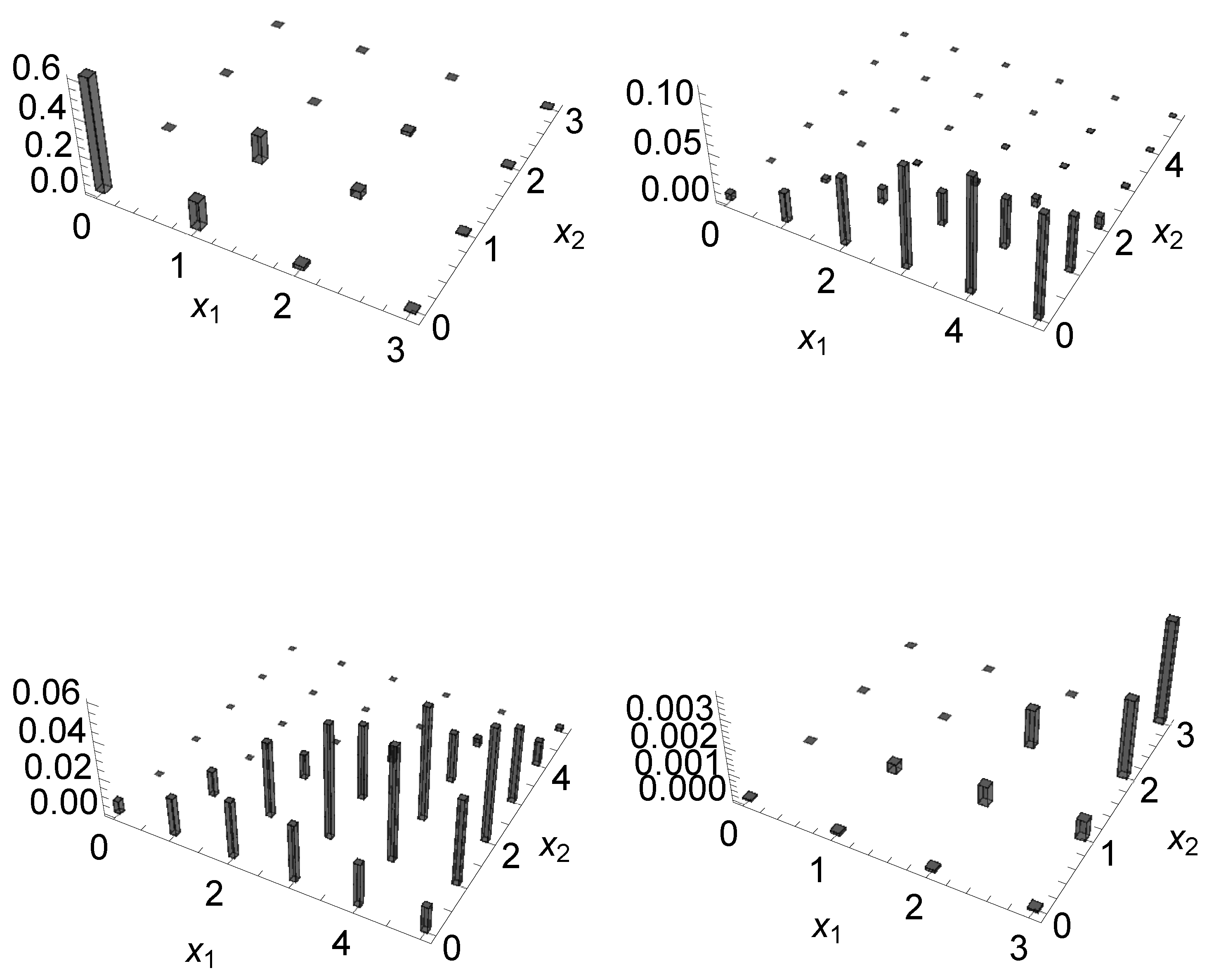
Below in

Table 1. Observed (in bold) and expected frequencies for threshold value $\psi =\$1000$.

	${\mathit{X}}_2$	0	1	2	3	4	Total
${\mathit{X}}_1$
0		63,232					63,232
		63,098.00					63,098.00
		63,279.50					63,279.50
1		2551	1782				4333
		2713.21	1874.01				4587.22
		2518.34	1768.19				4286.53
2		109	114	48			271
		58.33	80.58	27.83			166.74
		101.75	116.10	54.15			272
3		5	6	6	1		18
		0.83	1.73	1.20	0.27		4.03
		4.26	6.14	4.66	1.81		16.87
4		1	0	0	1	0	2
		0.01	0.02	0.01	0.02	0.01	0.07
		0.18	0.31	0.29	0.18	0.06	1.02
Total		65,110	1902	54	2	0	67,856
		65,870.38	1956.34	29.04	0.29	0.01	67,856.06
		65,904.03	1890.74	59.10	1.99	0.06	67,856.00

, the observed (in bold) and expected frequencies with the threshold value for the claims assumed to be $\psi =\$1000$ are shown. For each entry, observed frequencies (top row in bold), expected frequency under the basic model (given by using (1) in the middle row), and mixture model (bottom row), obtained by using (12), are illustrated. Furthermore, the marginal observed and expected frequencies are in the far right column and in the bottom row for $X_1$ and $X_2$, respectively. The cells in this table are grouped to comply with the rule of five when applying the ${\chi }^2$ test.

Similarly,

Table 2. Observed (in bold) and expected frequencies for threshold value $\psi =\$3000$.

	${\mathit{X}}_2$	0	1	2	3	4	Total
${\mathit{X}}_1$
0		63,232					63,232
		63,098.00					63,098.00
		63,279.50					63,279.50
1		3576	757				4333
		3817.42	769.79				4587.21
		3554.25	732.28				4286.53
2		216	44	11			271
		115.48	46.57	4.69			166.74
		198.16	54.75	19.09			272
3		12	4	2	0		18
		2.33	1.41	0.28	0.01		4.03
		11.13	3.47	1.62	0.64		16.86
4		2	0	0	0	0	2
		0.03	0.03	0.01	0.00	0.00	0.07
		0.63	0.21	0.11	0.06	0.02	1.03
Total		67038	805	13	0	0	67,856
		67,033.26	815.80	4.98	0.01	0.00	67,856.05
		67,043.67	790.71	20.82	0.70	0.02	67,856.00

exhibits the observed and expected frequencies when the threshold amount was $\psi =\$3000$. Again, the cells are combined to comply with the rule of five. As can be seen, the fitting values obtained by using the mixture model were much more flexible since it incorporated heterogeneity among policyholders via the prior distributions, and it also provided a better fit to the data than those ones computed under the basic model for both thresholds.

Maximum likelihood estimation was used in both cases. It is convenient to point out that in the case of the mixture model, it was proven that directly maximizing the logarithm of the log-likelihood function provided, as expected, the same results as using the EM algorithm shown in Appendix B of this work. Mathematica and WinRaTs were the two packages used in this case.

Parameter estimates, standard errors (in brackets), the maximum of the log-likelihood function, figures of the chi-squared test statistics, degrees of freedom (d.f.), and the p-value are exhibited in

Table 3. Parameter estimates (in brackets) and measures of model selection for the basic and mixture models without covariates.

	$\mathit{\psi }=\mathit{\$}1000$		$\mathit{\psi }=\mathit{\$}3000$
	Basic Model	Mixture Model	Basic Model	Mixture Model
${\widehat{\mu }}_1$	0.0727	0.0727	0.0727	0.0727
	(0.001)	(0.000)	(0.001)	(0.000)
${\widehat{\mu }}_2$	0.0297	0.0297	0.0122	0.0123
	(0.000)	(0.000)	(0.000)	(0.000)
${\widehat{\gamma }}_1$		15.900		15.900
		(0.000)		(0.000)
${\widehat{\gamma }}_2$		4.334		2.035
		(0.000)		(0.000)
${\ell }_{max}$	−21,346.561	−21,292.395	−20,301.926	−20,242.391
${\chi }^2$	>100	5.16	>100	2.09
d.f.	4	2	3	1
p-value	0.00%	7.58%	0.00 %	14.83%

for the basic and mixture models. Results under the threshold value first $\psi =\$1000$ are shown in the second and third columns and $\psi =\$3000$ in the last two columns. Virtually, the same estimates were obtained for parameters ${\mu }_1$ and ${\mu }_2$ under the basic and mixture models. Similarly, no changes were discernible in the estimates between the estimates for the two thresholds with the exemption of the estimate of parameter ${\gamma }_2$. In this case, it was observable that the estimate decreased when the threshold increased. By incrementing the threshold value, the fit to the data improved. The mixture model provided the best fit to the data in terms of the ${\chi }^2$ test statistic and the negative of the maximum of the likelihood function ${\ell }_{max}$. Note that the mixture model was not rejected at the 5% significance level for the two thresholds previously considered. It is important to note that, although the gain in terms of maximum of the log-likelihood function did not seem significant, the mixture model was preferable in terms of the ${\chi }^2$ test statistics since, unlike the basic one, it was not rejected at the 5% significance level (see the corresponding p-values) in either of the two thresholds mentioned above.

We now implement explanatory variables in our analysis. The following covariates were considered: gender of driver, vehicle body, driver’s area of residence, age of vehicle, and driver’s age category. In addition, an intercept was also included in the study. Details about the codification of these variables can be found on the same website. Moreover, an offset variable (exposure, log of the time exposed to risk) was included in the linear predictor associated with the first variable.

Table 4. Parameter estimates and p-values associated with the Wald test for the mixture model including covariates.

	$\mathit{\psi }=1000$				$\mathit{\psi }=3000$
	Variable ${\mathit{X}}_1$		Variable ${\mathit{X}}_2$		Variable ${\mathit{X}}_1$		Variable ${\mathit{X}}_2$
Parameter	Estimate	p-Value	Estimate	p-Value	Estimate	p-Value	Estimate	p-Value
GENDER	−0.015	0.613	0.105	0.090	−0.022	0.467	0.220	0.007
BUS	0.244	0.610	−0.384	0.558	1.005	0.002	−1.386	0.208
CONVT	−0.562	0.342	−0.406	0.738	−0.525	0.364	0.890	0.461
COUPE	0.503	0.000	0.204	0.401	0.489	0.000	0.007	0.982
HDTOP	0.208	0.024	−0.427	0.026	0.181	0.049	−0.682	0.011
MCARA	0.766	0.003	−1.291	0.050	0.668	0.011	−1.495	0.152
MIBUS	0.098	0.514	0.292	0.342	0.018	0.905	−0.501	0.234
PANVN	0.124	0.335	−0.286	0.272	0.132	0.299	−0.415	0.223
RDSTR	0.131	0.856	−0.278	0.823	0.318	0.624	−1.143	0.672
SEDAN	0.063	0.098	−0.148	0.055	0.058	0.128	−0.348	0.001
STNWG	0.124	0.002	−0.150	0.076	0.107	0.010	−0.471	0.000
TRUCK	0.055	0.570	−0.040	0.835	0.056	0.560	−0.506	0.050
UTE	−0.100	0.152	−0.054	0.699	−0.111	0.110	−0.271	0.126
AREAA	−0.010	0.885	−0.194	0.152	−0.064	0.343	−0.108	0.001
AREAB	0.050	0.472	−0.207	0.132	−0.005	0.938	−0.571	0.004
AREAC	0.007	0.920	−0.293	0.027	−0.053	0.421	−0.496	0.035
AREAD	−0.110	0.144	−0.139	0.352	−0.171	0.021	−0.345	0.003
AREAE	−0.037	0.641	−0.125	0.420	−0.093	0.228	−0.572	0.293
VAGE1	0.187	0.000	−0.388	0.000	0.168	0.000	−0.271	0.000
VAGE2	0.219	0.000	−0.259	0.001	0.207	0.000	−0.619	0.009
VAGE3	0.098	0.013	−0.010	0.208	0.083	0.035	−0.275	0.283
AGE1	0.512	0.000	0.291	0.034	0.464	0.000	0.746	0.000
AGE2	0.328	0.000	0.032	0.795	0.286	0.000	0.274	0.118
AGE3	0.275	0.000	0.039	0.746	0.229	0.000	0.273	0.111
AGE4	0.243	0.000	−0.043	0.723	0.202	0.001	0.196	0.253
AGE5	0.030	0.656	−0.044	0.740	−0.013	0.843	−0.002	0.990
CONSTANT	−2.273	0.000	0.027	0.880	−2.156	0.000	−1.045	0.000
${\widehat{\gamma }}_1$	21.602	0.000			30.718	0.000
${\widehat{\gamma }}_2$	5.903	0.185			2.205	0.014

illustrates the estimates of the regressors for the mixture model associated with the random variables $X_1$ and $X_2$ again for a threshold of $\psi =\$1000$ and $\psi =\$3000$. In the first case, the explanatory variables hardtop (HDTOP), motorized caravan (MCARA), driver’s area of residence C (AREAC), age of Vehicles 1 and 2 (VAGE1 and VAGE2), and driver’s Age Category 1 (AGE 1) were statistically significant at the 5% significance level for the random variable total number of claims given that the claim size exceeded $\psi =\$1000$. Among these variables, only HDTOP, MCARA, VAGE1, VAGE2, and AGE1 were significant for both response variables. However, it is important to note that all these variables except for the regressors associated with AGE1 and AGE2, the sign of the estimates changed from positive to negative for claims above the threshold. Furthermore, the estimate of parameter ${\gamma }_1$ was statistically significant at the same nominal level. When the threshold value was increased up to $\psi =\$3000$, the number of significative variables above the threshold considerably grew since now, the intercept (CONSTANT), gender of driver (GENDER), HDTOP, SEDAN, station wagon (STNWG), TRUCK, AREAA, AREAB, AREAC, AREAD, VAGE1, VAGE2, and AGE1, were relevant. However, only CONSTANT, HDTOP, STNWG, AREAD, VAGE1, VAGE2, and AGE1 were significant for both dependent variables at the same nominal level. The regressors associated with the explanatory variables CONSTANT, AREAD, and the AGE1 had the same sign for claims below and above $\psi =\$3000$. The first two regressors were negatively correlated and the latter one positively correlated to the response variables, respectively. For the other regressors, once again, the sign of the estimates changed from positive to negative for claims above the threshold. Among the common statistically significant estimates for both threshold values, i.e., HDTOP, VAGE1, VAGE2, and AGE1, the same sign of the estimates in the variables $X_1$ and $X_2$ was observable. For the non-significant estimates, different signs were observed in the regressors. Furthermore, the estimates of parameters ${\gamma }_1$ and ${\gamma }_2$ were statistically significant at the same nominal level.

Similarly to the case previously considered, the fit to the data improved when covariates were incorporated in the model and when the threshold value enlarged.

Table 5. Parameter estimates (in brackets) and measures of model selection for the basic and mixture models with covariates.

	$\mathit{\psi }=\mathit{\$}1000$		$\mathit{\psi }=\mathit{\$}3000$
	Basic Model	Mixture Model	Basic Model	Mixture Model
$-{\ell }_{max}$	20,604.355	20,588.936	19,545.212	19,511.783
AIC	41,312.710	41,289.872	39,198.422	39,135.565
BIC	41,809.468	41,800.880	39,691.180	39,646.573
CAIC	41,863.468	41,856.880	39,745.180	39,702.573

exhibits the negative of the maximum of the likelihood function ($-{\ell }_{max}$), Akaike’s information criterion (AIC), the Bayesian information criterion (BIC), and the consistent Akaike’s information criterion (CAIC) for the basic and mixture regression models. A lower value of these measures of model selection was desirable. It was observable that the latter model was preferable to the former one.

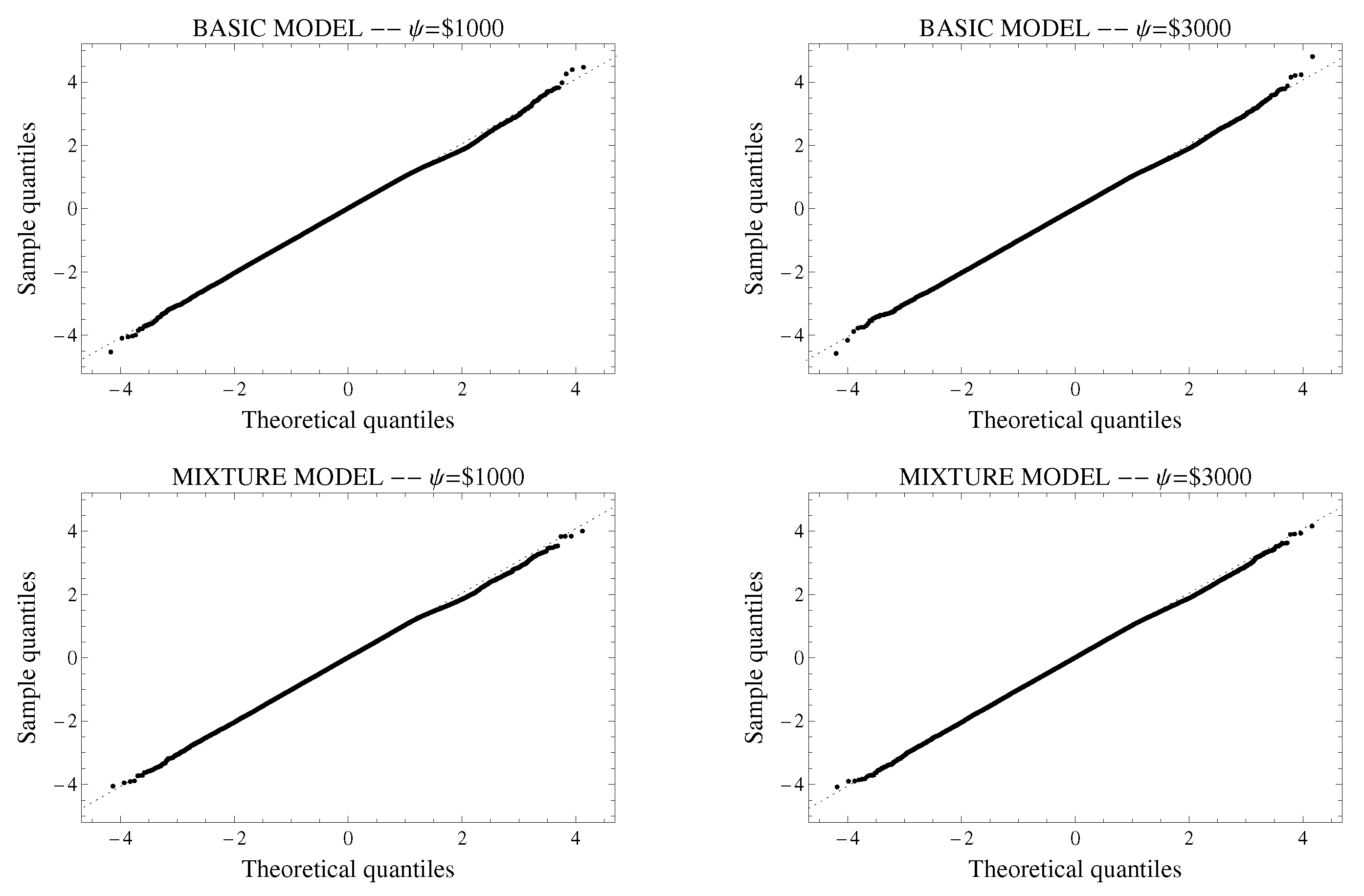
We plot the QQ-plots of the randomized quantile residuals to check for normality in Figure 2. The residuals for the basic regression models are shown in the top row and for the mixture regression model in the bottom row. Furthermore, models that use $\psi =\$1000$ as the threshold value are exhibited in the left column and $\psi =\$3000$ in the right-hand column. A perfect alignment with the 45${}^{\circ }$ line implies that the residuals are normally distributed. It was observable that the residuals for the larger threshold values adhered a little bit closer to the line, but these differences were not significant.

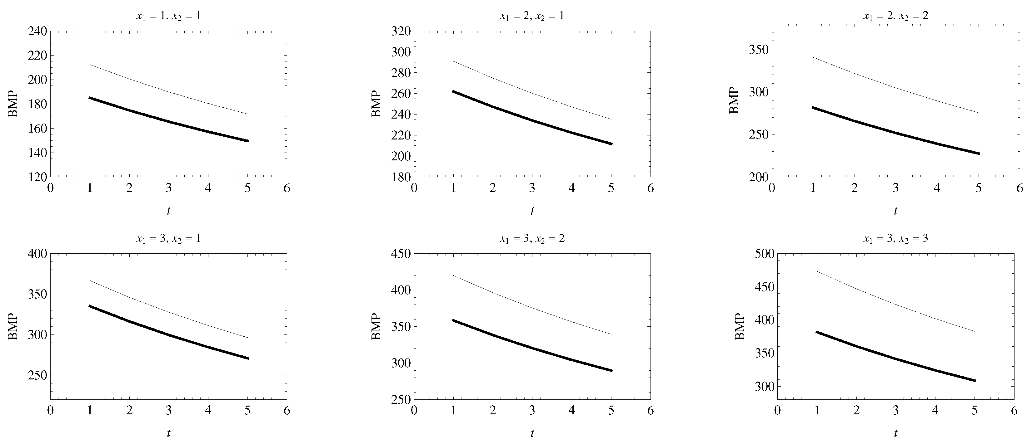
Figure 3 exhibits the bonus-malus premiums (BMP) for the mixture model without covariates. Here, $x_1$ is the total number of claims when $x_2$ claims out of $x_1$ have a size larger than $\psi$. In each chart, the thick line represents $\psi =\$1000$, and the thin line denotes $\psi =\$3000$. It was noticeable that the BMP decreased with the time period when the observed pair $x_1$ and $x_2$ was fixed for the two thresholds considered. The BMP was consistently lower when the threshold $\psi$ decreased. Although for both values of $\psi$, the premium charged increased when $x_1$ and $x_2$ grew, the premium paid also increased with $x_2$ when $x_1$ was fixed.

Figure 4 illustrates the bonus-malus premiums (BMP) to be charged to the subgroup of policyholders with SEDAN and AREAA. In this case, we used the mixture regression model including the rest of the explanatory variables and the exposure. Similar conclusions could be drawn from this set of graphs. Again, the BMP was persistently lower when the threshold $\psi$ decreased. The premium charged increased when $x_1$ and $x_2$ grew for either value of $\psi$; moreover, the premium paid rose with $x_2$ when $x_1$ was held fixed. As compared to the premiums obtained under this regression model were way higher than those ones derived before, this could be surely explained by the small sample size used to estimate regressors and also for the incorporation of the offset variable that without any doubt affected the individual average number of claims and the probability of making a claim higher than the threshold. Other different subgroups of policyholders could also be used for tarification purposes; however, for some of these classes, non-reliable estimates were obtained due to the very low sample size.

Computations in the Compound Model

Although it is customary to calculate the bonus-malus premium based on the variable number of claims (it is usually considered that once a loss has occurred, the company does not have the ability to model the amount corresponding to the loss), some attempts have been made to implement the severity in the calculation of the premium. Some works related to this topic are Frangos and Vrontos (2001); Pinquet (1998), and Gómez-Déniz et al. (2014), among others. As the practitioner wishes to calculate the premium using both variables, it is useful to rely on the composite collective model. Similarly to the univariate case, the bivariate compound distributions for the aggregate claim size random variable can be simply derived as follows:

$$g(y_1,y_2)=\sum _{x_1,x_2=0}^{\infty }{p}_{x_1,x_2}{f}_1^{*x_1}\left(y_1\right)f_2^{*x_2}\left(y_2\right),$$

(16)

and this is the the joint probability density function of $(Y_1,Y_2)=\left(S_1,S_2,\right)$, where $S_1={\sum }_{i=0}^{X_1}{Y}_{1i}$, $S_2={\sum }_{i=0}^{X_2}{Y}_{2i}$ are the aggregate severities, $Y_1$ and $Y_2$ being mutually independent and also independent of $(X_1,X_2)$ with probability functions (discrete or continuous) $f_1\left(y_1\right),f_2\left(y_2\right)$, respectively, with $x_1$ and $x_2$-fold convolutions $f_1^{*x_1}\left(y_1\right)$ and $f_2^{*x_2}\left(y_2\right)$, respectively. General expressions for $E\left(S\right)$, $var\left(S\right)$ and $cov(S_1,S_2)$, where $S=S_1+S_2$, were provided in Partrat (1994).

Recursion for bivariate count distributions and their compound distributions given in the form (16) have been previously considered in the actuarial literature; see Theorem 2.1. in Hesselager (1996). Other similar recursions can be found in Vernic (1997); Walhin and Paris (2000); Walhin and Paris (2001); Sundt (2002), and Sundt and Vernic (2009), among others. Moreover, bivariate recursions are useful in prediction problems involving the conditional $g\left(y\right|x)$ of Y, given $X=x$; see Hesselager (1996) for more details.

Let us now assume that the random variables $X_1$ and $X_2$ represent two kinds of claims, for instance bodily injury and material damage, or as in our study, claims below and above a threshold $\psi$.

The fact that the probability generating function of (1) is analytically obtained helps us to derive the probability generating function of the joint random variable $(X_1\left(d_1\right),X_2\left(d_2\right))$ for $d_i$, which can be deduced in type $i(i=1,2)$ claim amounts. Here, $X_i\left(d_i\right)$ is the random variable corresponding to the yearly frequency of type i claims exceeding $d_i$. The work in Partrat (1994) then showed that the probability generating function of the random variable $(X_1\left(d_1\right),X_2\left(d_2\right))$ is given by:

$$\begin{array}{ccc}\hfill G_{X_1\left(d_1\right),X_2\left(d_2\right)}(s_1,s_2)& =& G_{X_1,X_2}((1-F_1\left(d_1\right))s_1\hfill \\ & & +F_1\left(d_1\right),(1-F_2\left(d_2\right))s_2+F_2\left(d_2\right)),\hfill \end{array}$$

where $F_1$ and $F_2$ are the cumulative distribution functions of the random variables $Y_1$ and $Y_2$, respectively; while the probability generating function of the random variable $X(d_1,d_2)$, with $X=X_1+X_2$, is given by:

$$\begin{array}{c}\hfill G_{X(d_1,d_2)}(s_1,s_2)=G_{X_1,X_2}((1-F_1\left(d_1\right))s_1+F_1\left(d_1\right),(1-F_2\left(d_2\right))s_2+F_2\left(d_2\right)).\end{array}$$

6. Final Comments

In this paper, a flexible bivariate count data regression model that let us distinguish between different types of claims according to the claim size was introduced. Besides, it allowed us to examine the factors that affect the number of claims above and below a given claim size threshold. By means of a mixture regression model, the individual claim size and other risk factors such as gender, type of vehicle, driving area, or age of the vehicle could be used to compute credibility bonus-malus premiums. Extensions of this work includes a simple modification of this model to differentiate between more than two claims in the line of the work provided in Gómez-Déniz and Calderín-Ojeda (2018). Besides, a similar model can be simply implemented when the number of claims is distributed according to a negative binomial distribution. A study of this nature would be a possible extension of this work.

References

1. Bapat, Ravindra B. 1988. Discrete multivariate distributions and generalized log-concavity. Sankhya¯: The Indian Journal of Statistics, Series A 1: 98–110. [Google Scholar]
2. Barndorff-Nielsen, Ole. 1973. Unimodality and exponential families. Communications in Statistics-Theory and Methods 1: 189–216. [Google Scholar]
3. Bermúdez, Lluís. 2009. A priori ratemaking using bivariate Poisson regression models. Insurance: Mathematics and Economics 44: 135–41. [Google Scholar] [CrossRef] [Green Version]
4. Bermúdez, Lluís, and Dimitris Karlis. 2017. A priori ratemaking using bivariate Poisson models. Scandinavian Actuarial Journal 2: 148–58. [Google Scholar] [CrossRef] [Green Version]
5. Bonsdorff, Heikki. 2005. On asymptotic properties of Bonus-Malus systems based on the number and on the size of the claims. Scandinavian Actuarial Journal 4: 309–20. [Google Scholar] [CrossRef]
6. Bühlmann, Hans, and Alois Gisler. 2005. A Course in Credibility Theory and Its Applications. Berlin: Springer. [Google Scholar]
7. Cameron, Colin, and Pravin K. Trivedi. 1998. Regression Analysis of Count Data. Cambridge: Cambridge University Press. [Google Scholar]
8. De Jong, lPiet, and Gillian H. Heller. 2008. Generalized Linear Models for Insurance Data. Cambridge: Cambridge University Press. [Google Scholar]
9. Denuit, Michel, Xavier Marèchal, Sandra Pitrebois, and Jean F. Walhin. 2009. Actuarial Modelling of Claim Counts Risk Classification, Credibility and Bonus-Malus Systems. New York: John Wiley & Sons. [Google Scholar]
10. Dionne, Georges, and Charles Vanasse. 1989. A generalization of actuarial automobile insurance rating models: The negative binomial distribution with a regression component. ASTIN Bulletin 19: 199–212. [Google Scholar] [CrossRef]
11. Frangos, Nikolaos, and Spyridon Vrontos. 2001. Design of optimal bonus-malus systems with a frequency and a severity component on an individual basis in automobile insurance. ASTIN Bulletin 31: 1–22. [Google Scholar] [CrossRef] [Green Version]
12. Gerber, Hans U. 1979. An Introduction to Mathematical Risk Theory. Homewood: Huebner Foundation Monograph. [Google Scholar]
13. Gómez-Déniz, Emilio. 2008. A generalization of the credibility theory obtained by using the weighted balanced loss function. Insurance: Mathematics and Economics 42: 850–54. [Google Scholar] [CrossRef]
14. Gómez-Déniz, Emilio. 2016. Bivariate credibility bonus-malus premiums distinguishing between two types of claims. Insurance: Mathematics and Economics 70: 117–24. [Google Scholar] [CrossRef]
15. Gómez-Déniz, Emilio, and Enrique Calderín-Ojeda. 2018. Multivariate credibility in bonus-malus systems distinguishing between different types of vlaims. Risks 6: 34. [Google Scholar] [CrossRef] [Green Version]
16. Gómez-Déniz, Emilio, Agustín Hernández, and María P. Fernández. 2014. Computing credibility bonus-malus premiums using the total claim amount distribution. Hacettepe Journal of Mathematics and Statistics 43: 1047–61. [Google Scholar]
17. Heilmann, Wolf R. 1989. Decision theoretic foundations of credibility theory. Insurance: Mathematics and Economics 8: 75–95. [Google Scholar] [CrossRef]
18. Hesselager, Ole. 1996. Recursions for certain bivariate counting distributions and their compound distributions. ASTIN Bulletin 26: 35–52. [Google Scholar] [CrossRef] [Green Version]
19. Johnson, Norman, Samuel Kotz, and Narayanaswamy Balakrishnan. 1997. Discrete Multivariate Distributions. New York: Wiley. [Google Scholar]
20. Khatri, Chinubhai G. 1983a. Multivariate discrete exponential distributions and their characterization by Rao-Rubin condition for additive damage model. South African Statistical Journal 17: 13–32. [Google Scholar]
21. Khatri, Chinubhai G. 1983b. Multivariate discrete exponential family of distributions. Communications in Statistics-Theory and Methods 12: 877–93. [Google Scholar] [CrossRef]
22. Klugman, Stuart A., Harry H. Panjer, and Gordon E. Willmot. 2008. Loss Models: From Data to Decisions, 3rd ed. New York: Wiley. [Google Scholar]
23. Kocherlakota, Subrahmaniam, and Kathleen Kocherlakota. 1992. Bivariate Discrete Distributions. New York: Marcel Dekker. [Google Scholar]
24. Lee, Mei-Ling T. 1996. Properties and applications of the Sarmanov family of bivariate distributions. Communications in Statistics-Theory and Methods 25: 1207–22. [Google Scholar]
25. Louis, Thomas A. 1982. Finding the observed information matrix when using the EM algorithm. Journal of the Royal Statistical Society. Series B 44: 226–33. [Google Scholar]
26. Partrat, Christian. 1994. Compound model for two dependent kinds of claims. Insurance: Mathematics and Economics 15: 219–31. [Google Scholar] [CrossRef]
27. Pedersen, Jean G. 1975. On strong unimodality of two-dimensional discrete distributions with applications to M-Ancillarity. Scandinavian Journal of Statistics 2: 99–102. [Google Scholar]
28. Pinquet, Jean. 1998. Designing optimal bonus-malus systems from different types of claims. ASTIN Bulletin 28: 205–20. [Google Scholar] [CrossRef] [Green Version]
29. Ragulina, Olena. 2011. Bonus-malus systems with different claim types and varying deductibles. Modern Stochastics: Theory and Applications 4: 141–59. [Google Scholar] [CrossRef]
30. Rolski, Tomasz, Hanspeter Schmidli, Volker Schmidt, and Jozef Teugel. 1999. Stochastic Processes for Insurance and Finance. Hoboken: John Wiley & Sons. [Google Scholar]
31. Sundt, Bjoern. 2002. Recursive evaluation of aggregate claims distributions. Insurance: Mathematics and Economics 30: 297–322. [Google Scholar] [CrossRef]
32. Sundt, Bjoern, and Raluca Vernic. 2009. Recursions for Convolutions and Compound Distributions with Insurance Applications. New York: Springer. [Google Scholar]
33. Vernic, Raluca. 1997. On the bivariate generalized Poisson distribution. ASTIN Bulletin 27: 23–31. [Google Scholar] [CrossRef] [Green Version]
34. Walhin, Jean F., and John Paris. 2000. Recurs1ve formulae for some bivariate counting distributions obtained by the trivariate reduction method. ASTIN Bulletin 30: 141–55. [Google Scholar] [CrossRef] [Green Version]
35. Walhin, Jean F., and John Paris. 2001. The mixed bivariate Hofmann distribution. ASTIN Bulletin 31: 127–42. [Google Scholar] [CrossRef] [Green Version]
Figure 1. Joint probability mass functions of the bivariate discrete distribution proposed for selected values of the parameters. From top to bottom and left to right, we have: ( μ 1 , μ 2 ) = ( 0.5 , 0.25 ) , ( μ 1 , μ 2 ) = ( 5 , 0.5 ) , ( μ 1 , μ 2 ) = ( 5 , 2 ) , and ( μ 1 , μ 2 ) = ( 10 , 8 ) .
Risks 08 00020 g001
Figure 2. QQ-plots of the randomized quantile residuals for the basic (top) and mixture (bottom) regression models for ψ = $ 1000 (left) and ψ = $ 3000 (right) threshold values.
Risks 08 00020 g002
Figure 3. Bayesian bonus-malus premiums under the mixture model without covariates for x 1 claims when there are x 2 claims with a claim size larger than ψ . The thick line represents ψ = $ 1000 , and the thin line represents ψ = $ 3000 . BMP, bonus-malus premiums.
Risks 08 00020 g003
Figure 4. Bayesian bonus-malus premiums under the mixture model with covariates for x 1 claims when there are x 2 claims with a claim size larger than ψ . The thick line represents ψ = $ 1000 , and the thin line represents ψ = $ 3000 . This chart corresponds to the the subgroup of policyholders with SEDAN and AREAA.
Risks 08 00020 g004