Article

Delta Boosting Implementation of Negative Binomial Regression in Actuarial Pricing

Department of Statistics and Actuarial Science, The University of Hong Kong, Pokfulam Road, Hong Kong
Risks 2020, 8(1), 19; https://doi.org/10.3390/risks8010019
Submission received: 10 January 2020 / Revised: 3 February 2020 / Accepted: 7 February 2020 / Published: 19 February 2020

Abstract

:
This study proposes an efficacious approach to analyze the over-dispersed insurance frequency data as it is imperative for the insurers to have decisive informative insights for precisely underwriting and pricing insurance products, retaining existing customer base and gaining an edge in the highly competitive retail insurance market. The delta boosting implementation of the negative binomial regression, both by one-parameter estimation and a novel two-parameter estimation, was tested on the empirical data. Accurate parameter estimation of the negative binomial regression is complicated with considerations of incomplete insurance exposures, negative convexity, and co-linearity. The issues mainly originate from the unique nature of insurance operations and the adoption of distribution outside the exponential family. We studied how the issues could significantly impact the quality of estimation. In addition to a novel approach to simultaneously estimate two parameters in regression through boosting, we further enrich the study by proposing an alteration of the base algorithm to address the problems. The algorithm was able to withstand the competition against popular regression methodologies in a real-life dataset. Common diagnostics were applied to compare the performance of the relevant candidates, leading to our conclusion to move from light-tail Poisson to negative binomial for over-dispersed data, from generalized linear model (GLM) to boosting for non-linear and interaction patterns, from one-parameter to two-parameter estimation to reflect more closely the reality.

1. Introduction

The rising awareness among consumers about safety concerns has propelled them to buy insurance products with zeal and consistency, resulting in a barrage of insurance data in the retail insurance industry. The generally competitive markets of the retail insurance business have made it imperative for insurers to retain their customer base along with gaining an edge in the highly competitive retail insurance market. However, for actuaries and insurers to remain relevant in the insurance domain, a necessary evolution is required on their part to revamp the fundamentals of data collection and processing, identify novel rate-making and underwriting techniques and align those elements to better anticipate changes in the business circumstances. To deflect the underwriting risks and analyze the over-dispersed insurance frequency data adeptly, actuaries have been developing actuarial rate-making model with robust mathematical and statistical concepts like generalized linear models (Werner and Modlin 2010), generalized additive models (Lee and Antonio 2015), Markov chain Monte Carlo and Bayesian inference Using Gibbs Sampling (Scollnik 2001), neural networks (Lee and Antonio 2015), decision trees (Lee and Antonio 2015), and boosting machines (Lee and Lin 2015). Contrary to the pursuit of predictive risk models through complex machine learning, Casualty Actuarial and Statistical Task Force (2019) depicts principles that suggest the deployment of candid and efficient algorithms to enable more effective scrutiny for regulators and the management of insurers. It further recommends the predictive models be intuitive for pricing, and straightforward for system integration as these predictive algorithms can help return customer’s premium queries within a fraction of a second (Majumdar et al. 2019). In the era of digital experience, a transparent and seamless experience is imperative. The purpose of this study was to formulate and apply the novel actuarial rate-making methodology with special consideration on incomplete exposures abundant in real-life insurance frequency data and the negative convexity and co-linearity due to the adoption of the negative binomial distribution, along with comparing it against competitive modeling techniques.
We reviewed the literature of related works in Section 2. Section 3 started with the introduction of the core components of our proposed algorithm, the delta boosting machine and negative binomial regression. Although mainly used as one-parameter regression, the negative binomial is a two-parameter distribution. Section 4 first characterized the more popular one-parameter regression implemented in the delta boosting machine and Section 5 relaxed the assumption of the fixed shape parameter and detailed the mathematics in deriving the algorithm for simultaneous estimation of both scale and shape parameters. We continued to identify the risk of naive deployment of machine learning in rate-making as insurance data is filled with incomplete exposures. As negative binomial is not a member of the two-parameter exponential family, some features that are beneficial in regression are not present by default. We studied the risk introduced in the two-parameter estimation and proposed an arrangement to address the concerns.
The objective of Section 6 is to put the algorithm into the test with real-life data and compare the implementation with other competitive and related modeling candidates. Common diagnostics were utilized to set as benchmarking tools for comparison.
Section 7 concluded the paper with key insights from this study and offered directions on a potential area for further exploration.

2. Literature Review

The frequency–severity method, which involves separate consideration of frequency and severity (Anderson et al. 2007; Henckaerts et al. 2019) to calculate the indicated cost, is one of the two fundamental actuarial pricing processes. The cost calculations are achieved by multiplying the conditional expectation of severity with expected claim frequency. Henceforth, the frequency modeling of claims represents an essential step in non-life insurance rate-making. A frequency regression analysis permits the identification of risk factors and the prediction of the expected frequency of claims given risk characteristics (Boucher et al. 2009; Ridout et al. 1998; Yip and Yau 2005). The Poisson regression is a member of generalized linear models (GLMs) and was first developed by Nelder and Wedderburn (1972), detailed later in Gourieroux et al. (1984a, 1984b) and Teugels and Vynckie (1996) as the modeling archetype of claim frequency. Gagnon et al. (2008) described in the trauma research of behavioral outcomes, where Poisson regression provided readily interpretable results as rate ratios when applied to the count data.
Despite its popularity, the assumption of equality in observations’ mean and variance limits its application on the over-dispersed insurance frequency data (Boucher et al. 2009; Ridout et al. 1998; Yip and Yau 2005), in which the variance is generally higher than the expectation.
Several studies have shown a considerable improvement in precision by switching from Poisson to the alternative heavier tailed extension like negative binomial, quasi-Poisson, and zero-inflated regression (ZIP)(Ismail and Jemain 2007; Naya et al. 2008; Ver Hoef and Boveng 2007). The aforementioned distributions are either compound or mixture of Poisson. For instance, Breslow (1990) demonstrated using Monte Carlo simulation methods, a process of random sampling to estimate numerically unknown parameters, quasi-likelihood models can produce approximately unbiased estimates of the regression coefficients.  Ver Hoef and Boveng (2007) illustrated the restriction of Poisson in modeling count data in ecology and suggested relative merits in quasi-Poisson regression and negative binomial regression over Poisson. When tests were conducted on the motor claim insurance frequency data, the negative binomial model was found to correct the overdispersion and presented a better fit for the data (David and Jemna 2015). In  Naya et al. (2008), the authors compared the performance of Poisson and ZIP models under four simulation scenarios to analyze field data and established that the ZIP models gave better estimates than the Poisson models.
Negative binomial and ZIP are both extensions to Poisson (Lim et al. 2014; Teugels and Vynckie 1996), featuring inflated variances for any given expectations, and are particularly desirable for insurance pricing application (Teugels and Vynckie 1996). However, the ZIP model has a complicated output representation, with a combination of logistic and log-link transformation, that restricts its practical application whereas the parameters of negative binomial regression are both log-link and hence multiplicative. It offers a simpler real-life deployment and parameter interpretation.
Utilizing machine learning for predictive modeling enhances the pricing model validity through the GLM, which is a preeminently popular technique in actuarial practice owing to its strong statistical foundation and simplicity (Haberman and Renshaw 1996). Nevertheless, actuaries are provoked to pursue more reliable actuarial pricing models to gain a competitive edge in highly competitive markets. In Wuthrich and Buser (2019), various techniques were implemented including Adaboost, gradient boosting, regression tree boosting, GLM and generalized additive model (GAM) for a suitable non-life insurance actuarial pricing model. The authors summed up that the generalized additive model was able to outperform the generalized linear model for non-log-linear components. Similarly, Lee and Antonio (2015) and Henckaerts et al. (2019) compared the performance of GLM, GAM, bagging, random forest, and Gradient boosting (GB). When full tariff insurance plans were created, gradient boosting outperformed GLMs allowing the insurers to form profitable portfolios along with guarding them against any adverse risk selection. Gradient boosting algorithm outperformed Tweedie GLM when empirical tests were conducted by implementing it on the flexible non-linear Tweedie model, this method generated a more accurate insurance premium predictions (Yang et al. 2018). Thomas et al. (2018) elaborated that when a gradient boosting algorithm was implemented on GAMLSS i.e., generalized additive models for location, scale and size to generate boosted GAMLSS, it increased the flexibility of variable selection, time efficiency, and fewer boosting iterations were needed.
Lee and Lin (2015) introduced a novel modeling approach called delta boosting (DB) which is a forward stage-wise additive model that reduces the loss at each iteration and helps in enhancing the predictive quality. Instead of relying on the negative gradient as in the case for GB, DB adopts the loss minimizer of the basis. The commonly adopted modeling approach is to assume the over-dispersion parameter to be given or estimated through moment matching or maximum likelihood (JO 2007 and reference therein).
Exposure is the basic unit of risk that underlies the insurance premium and is heavily analyzed in traditional actuarial studies on aggregated data. It is a concept fairly unique to actuarial science. For example, written exposures, earned exposures, unearned exposures and in-force exposures (Werner and Modlin 2010) are defined for specific purposes. However, except for De Jong and Heller (2008) where simple yet effective handling of exposure for Bernoulli and Poisson is proposed, there has been little research on the optimal handling of incomplete exposures.

3. Delta Boosting Implementation of Negative Binomial Regression

The negative binomial distribution, a member of mixed Poisson, offers an effective way to handle over-dispersed insurance frequency data whereas DB is a member of boosting family which uses individual loss minimizers instead of gradients as the basis of regression. In this study, an adapted negative binomial regression implemented by the delta boosting algorithm is empirically tested by applying it to the real-time insurance frequency data.
The mathematical illustrations and proofs rely heavily on notations. To facilitate the discussion, all the key notations used in the paper are defined in Table 1.

3.1. Notation

The mathematical illustrations and proofs involve heavily on notations. To facilitate the discussion, all the key notations used in the paper are defined in Table 1.

3.2. Generic Delta Boosting Algorithms

Introduced in Lee and Lin (2015), delta boosting, a close sibling of gradient boosting, is a ensembling technique that consists of three main steps: basis, regression and adjust (Algorithm 1).
Loss functions are the ex-ante belief in evaluating the cost of inaccurate estimation (Lee and Lin 2018). Friedman (2001) studied the common choices of loss functions including mean-squared errors, mean-absolute errors or the negative log-likelihood of assumed distribution. This paper adopted the last option and compare the loss under Poisson and the negative binomial distribution respectively. In addition, practitioners also find appending penalty functions that temper the magnitudes of parameters helpful to address the overfitting problem Girosi et al. (1995).
There are two remarks in the delta boosting machine proposed in Lee and Lin (2015). First, DB is the optimal boosting member for many popular distributions including Poisson, Gamma, Tweedie, normal, Huber and more. Second, as  δ and Δ are designed such that the adjust step can be integrated with r e g r e s s i o n , the calculation is more efficient.
Algorithm 1 Delta boosting for a single parameter estimation.
  • Initialize F 0 ( x ) to be a constant, F 0 ( x ) = argmin β i = 1 M Φ ( y i , β )
  • For t = 1 to T Do
    (a)
    Basis : Compute the individual loss minimizer as the working response
    δ i = argmin s Φ ( y i , F ^ t 1 ( x i ) + s ) , i = { 1 , , M }
    Apply strictly monotonic transformation κ ( · ) on δ if necessary.
    (b)
    Regression : Obtain a t = argmin a i = 1 M i N j Φ ( y i , F t 1 ( x i ) + Δ j h ( x i ; a ) ) with Δ j defined in Table 1
    (c)
    Adjust : It is integrated with Regression step with β t , a t = Δ j for i N j .
    (d)
    Update F t ( x i ) = F t 1 ( x i ) + β t , a t h ( x i ; a t )
  • End For
  • Output F ^ ( x i ) = F ^ T ( x i )

3.3. Asymptotic DBM

The condition for DB to be optimal does not apply in the case of negative binomial as it does not meet the condition required. To cope with this, Lee and Lin (2015) offers an asymptotic alternative that is asymptotically optimal as the iteration grows. The sorting basis and the adjustment factor are replaced by δ * and Δ * respectively which are defined as follow
δ i * = Φ ( y i , F t 1 ( x i ) ) Φ ( y i , F t 1 ( x i ) ) Δ j * = i N j Φ ( y i , F t 1 ( x i ) ) i N j Φ ( y i , F t 1 ( x i ) ) ,
where N j stands for the j-th node of partition. We can also establish a relation between Δ * and δ *   through
Δ j * = i N j Φ ( y i , F t 1 ( x i ) ) δ i * i N j Φ ( y i , F t 1 ( x i ) ) .
For common regression with Poisson, Bernoulli or Gaussian distribution, Φ ( y i , F t 1 ( x i ) ) represents the variance of the sufficient statistics and are always positive. Thus, we can view Δ * as a weighted average of δ * with the convexity of the loss function. In the rest of the paper, we assume the base learner to be a 2-node stunt without loss of generality.

3.4. Negative Binomial Regression

The negative binomial regression, defined as a posterior distribution of Poisson with gamma as the secondary distribution proffers an efficacious way of handling discrete data where the distribution variance is greater than its mean.
Assume Y Poisson ( λ ) where λ Gamma ( α , β ) , then
P ( Y = k ) = 0 λ k e λ k ! λ α 1 e λ / β β α Γ ( α ) d λ = 0 λ k + α 1 e λ ( 1 + 1 / β ) k ! β α Γ ( α ) d λ = Γ ( α + k ) k ! Γ ( α ) 1 β + 1 α β β + 1 k .
It is trivial that E ( Y ) = α β and V a r ( Y ) = α β ( 1 + β ) , implying V a r ( Y ) > E ( Y ) . Thus, the negative binomial distribution is over-dispersed is more suitable than Poisson, for the insurance frequency data modeling where excessive zeros are common.
Both α and β are limited to be positive. The common regression practice is to impose a log-link transformation so that the transformed parameters can take any real numbers. In this paper, we will denote G and F to be the transformed parameters respectively so that
α ( x ) = e G ( x ) , α ^ ( x ) = e G ^ ( x ) β ( x ) = e F ( x ) , β ^ ( x ) = e F ^ ( x ) .
For negative binomial regression, the loss function, Φ ( y , G ( x ) , F ( x ) ) , is set to be the negative log-likelihood of the distribution.
Φ ( y , G ( x ) , F ( x ) ) = i = 1 M log ( P ( Y i = y i | x i ) ) = i = 1 M ψ ( e G ( x i ) + y i ) + ψ ( e G ( x i ) ) y i F ( x i ) + ( y i + e G ( x i ) ) log ( e F ( x i ) + 1 ) .
Various regression approach can be used to estimate F ( x ) and G ( x ) . In GLM, F ( x i ) is approximated in the form w 0 + j = 1 K w j x i j whereas the GAM approximation of F ( x i ) is w 0 + j = 1 K f i ( x i j ) .

4. Delta Boosting Implementation of One-Parameter Negative Binomial Regression

In negative binomial regression, it is a common practice to assume that α is identical for all observations. The estimation of α can be done through maximum likelihood estimate or moment matching, and also can be done upfront or alternately with β during the regression. In this subsection, we derive the functional form of F ^ ( x ) through the DB approach assuming a reliable estimate of α is provided.

4.1. Adaptation to Partial Exposure

In personal insurance, most of the data is structured with partial exposures, which means that the policies are not recorded in a complete policy term, normally 1 year. It can be due to clients’ actions (e.g., mid-term changes of policy or mid-term cancellation), regulatory changes (making the data before and after the changes exhibit different behaviors), business actions changing the composition of clients or even simply artificial data processing (e.g., calendar year cut-off for statutory reserving valuation and accounting purposes). Table 2 is an illustration of a policy recorded in the actuarial database.
A single policy is kept in nine entries for exposure in the year 2015 whereas the 10th entry shown in the table is for another policy term. The length of the period is captured as the exposure in each entry but it is sometimes possible to aggregate the entries having the same rating information. For example, the 2nd to 4th entries capture the same rating information and can be combined into one entry with the exposure of 0.189. However, the fifth entry indicates a change of vehicle and induces a change in the underlying risk of the insured. There is a significant amount of effective changes similar to the example and hence requiring a serious investigation of the topic on partial exposures. To the extent of authors’ knowledge, there is no research and publication about studying the optimal handling of partial exposures in machine learning.
By assumption of insurance pricing, the propensity on the incurring claims should be proportional to the length of the exposure. On the contrary, as long as the underlying risk factors do not change, the overall price in the same period should be identical regardless of whether the price is calculated annually or monthly or even artificial split. In Poisson regression, actuaries can take this assumption into account by simply considering the exposure as an offset due to the unique time homogeneity property of the Poisson process. However, the proper handling of exposure for other distributions may not be trivial.
We explore the outcome of applying the offset handling of incomplete exposure in negative binomial regression. As a simple illustration, we have one policy that is split artificially into i observations with w i ( i = 1 w i = 1 ) as the length of exposure. We have Y i Poisson ( λ i ) where λ i Gamma ( A i α , B i β ) and the effect of { A i = 1 , B i = w i } and { A i = w i , B i = 1 } are studied. The resulting loss function is:
Φ = i = 1 log 0 λ y i e λ y i ! λ A i α 1 e λ / ( B i β ) ( B i β ) A i α Γ ( A i α ) d λ = i = 1 log ( y i ! Γ ( A i α ) ) log ( Γ ( A i α + y i ) ) + i = 1 ( A i α + y i ) log ( B i β + 1 ) y i log ( B i β ) = i = 1 log ( y i ! Γ ( A i e G ) ) log ( Γ ( A i e G + y i ) ) + i = 1 ( A i e G + y i ) log ( B i e F + 1 ) y i ( F + log ( B i ) ) .
In the case where α is a constant, then the first summation is also a constant in the regression.
Φ F = i = 1 ( A i e G + y i ) B i e F B i e F + 1 y i = ( e G + y ) e F e F + 1 y , if { A i = w i , B i = 1 } i = 1 ( e G + y i ) w i e F w i e F + 1 y i , if { A i = 1 , B i = w i } .
In the case where { A i = w i , B i = 1 } , the inference is invariant to partitions, a desirable feature in this setting.
On the contrary, the inference in { A i = 1 , B i = w i } is not preserved. In such a setting, the expectation of the loss function, E ( Φ ) = i = 1 w i α β ^ w i β + 1 w i β ^ + 1 w i α β . If  β , β ^ or β β ^ are far from zero, there will be a significant divergence between the expectation of loss function between the full exposure and its split aggregate. In particular, β β ^ is generally significant at the beginning of iterations as β ^ is still a coarse estimate. This imposes a risk that the early, and important, search of predictive estimate can be ineffective.
Accordingly, we assign the offset factor to α in a single parameter regression. It is, in fact, against the mainstream assumption by popular R or Python libraries. GLM or GAM implementations of negative binomials do not assume the inclusion of offset in α and therefore for comparison, we will apply the offset on β for the GLM and GAM implementations.

4.2. Derivation of the Algorithm

We first derive the F ^ 0 ( x i ) by maximum likelihood estimation. With  w and w i defined as the exposure vector and exposure for observation i respectively,
F ^ 0 ( x i ) = argmin s Φ ( y , w α , s ) i = 1 M y i ( y i + w i α ) e F ^ 0 ( x i ) e F ^ 0 ( x i ) + 1 = 0 F ^ 0 ( x i ) = log i = 1 M y i i = 1 M w i α .
The running prediction after iteration t 1 is F ^ t 1 ( x ) . At iteration t, we first derive the individual delta
δ i * = y i ( y i + w i α ) e F ^ t 1 ( x i ) e F ^ t 1 ( x i ) + 1 ( y i + w i α ) e F ^ t 1 ( x i ) ( e F ^ t 1 ( x i ) + 1 ) 2 .
Without any loss of generality, we assume the base learner to be a two-node stunt, the simplest classification and regression tree with only left node and right node. For the left node, define the prediction as Δ L * , we have
Δ L * = i N L y i ( y i + w i α ) e F ^ t 1 ( x i ) e F ^ t 1 ( x i ) + 1 i N L ( y i + w i α ) e F ^ t 1 ( x i ) ( e F ^ t 1 ( x i ) + 1 ) 2 .
The partition is derived by searching the split point that maximizes the loss reduction. For the negative binomial regression, a loss is defined to be the negative log-likelihood. The loss reduction at iteration t is
Φ ( y , w α , F ^ t 1 ( x ) ) Φ ( y , w α , F ^ t ( x ) ) = i = 1 M Φ ( y i , w i α , F ^ t 1 ( x i ) ) Φ ( y i , w i α , F ^ t ( x i ) ) i N L Φ ( y i , α , F ^ t 1 ( x i ) ) Δ L 2 + i N R Φ ( y i , α , F ^ t 1 ( x i ) ) Δ R 2 = i N L ( y i + α ) e F ^ t 1 ( x i ) ( e F ^ t 1 ( x i ) + 1 ) 2 Δ L 2 + i N R ( y i + α ) e F ^ t 1 ( x i ) ( e F ^ t 1 ( x i ) + 1 ) 2 Δ R 2 ,
where ≈ denotes “asymptotically equal”. Algorithm 2 summarizes the above logistics.
Algorithm 2 Delta boosting for one-parameter negative binomial regression.
  • Initialize F ^ 0 ( x ) to be a constant, F ^ 0 ( x ) = log i = 1 N y i i = 1 M w i α
  • For t = 1 to T Do
    (a)
    Basis : Compute the individual loss minimizer as the working response
    δ i * = y i ( y i + w i α ) e F ^ t 1 ( x i ) e F ^ t 1 ( x i ) + 1 ( y i + w i α ) e F ^ t 1 ( x i ) ( e F ^ t 1 ( x i ) + 1 ) 2 , i = { 1 , , M }
    (b)
    Regression : Obtain a t = argmin a i N j Φ ( y i , F ^ t 1 ( x i ) + Δ j * h ( x i ; a ) ) with
    Δ j * = i N j y i ( y i + w i α ) e F ^ t 1 ( x i ) e F ^ t 1 ( x i ) + 1 i N j ( y i + w i α ) e F ^ t 1 ( x i ) ( e F ^ t 1 ( x i ) + 1 ) 2
    (c)
    Adjust : It is integrated with Regression step with adjustment equal to Δ * .
    (d)
    Update F ^ t ( x i ) = F ^ t 1 ( x i ) + Δ j * h ( x i ; a t ) for i N j .
  • End For
  • Output F ^ ( x i ) = F ^ T ( x i )

5. Delta Boosting Implementation of Two-Parameter Negative Binomial Regression

Except for the multinomial regression (Darroch and Ratcliff 1972), almost all research mentioned in Section 2 focused on the one-parameter estimation. In this section, we propose an extension to the moderated delta boosting algorithm earlier in Section 4 that allows simultaneous estimations of the shape and scale parameters in the negative binomial distribution. We will also walkthrough, in the rest of this section, the proposed adaptation we applied to address some key issues due to the relaxation of parameter assumption and the incomplete exposure phenomenon in insurance data.

5.1. Adaptation to Incomplete Exposure

Thanks to the forward stage-wise property in DB, the simultaneous regression of α and β is achievable. We define the estimate of α and β as α ^ and β ^ respectively.
Since α is no longer assumed to be constant, in addition to the consideration we made for β in Equation (3), we also studied the impact of incomplete exposure on the inference of α .
Differentiating the loss function by G,
Φ ( y , F , G ) G = i = 1 A i e G ( ψ ( A i e G ) ψ ( A i e G + y i ) + log ( B i e F + 1 ) ) = i = 1 ( w i e G ( ψ ( w i e G ) ψ ( w i e G + y i ) + log ( e F + 1 ) ) ) x x x if { A i = w i , B i = 1 } i = 1 e G ( ψ ( e G ) ψ ( e G + y i ) + log ( w i e F + 1 ) ) if { A i = 1 , B i = w i } = i = 1 ( w i e G ( ψ ( w i e G ) ψ ( w i e G + y i ) ) ) + e G log ( e F + 1 ) ) if { A i = w i , B i = 1 } K e G ψ ( e G ) i = 1 e G ( ψ ( e G + y i ) log ( w i e F + 1 ) ) if { A i = 1 , B i = w i } ,
where ψ ( x ) represents the digamma ( x ) . As stated in Section 4.1, Φ F is invariant under the partition. For  Φ G , the inference is also invariant if y < 2 , representing over 97% of the observation in the empirical data we deployed in Section 6 as most often an insured does not incur more than one accident in any exposure periods. In the case where y 2 , the inference will still stay the same if all incidence happened in the same exposure window. Otherwise, the aggregated loss gradient in Equation (5) is always larger than the full exposure equivalence.
In the case where { A i = 1 , B i = w i } , we concluded in Section 4.1 that the inference of Φ F is impacted by the way an observation is split to exposure. From Equation (5), the first term of Φ G grows by the number of splits and the second term also almost grows at the same rate as most of the responses are zero. On the contrary, the magnitude of the third term is
i = 1 e G log ( w i e F + 1 ) i = 1 e G w i e F = e G e F .
The asymmetric change of the three items imposes an adverse impact on the inference of α as the estimation varies materially by the choice of splitting observations although the splits are merely artificial for accounting purposes most of the time.
This analysis is propelling for us to apply the exposure as an offset to α in throughout this paper.

5.2. Derivation of the Algorithm

We first derive the F ^ 0 ( x i ) and G ^ 0 ( x i ) that minimize the loss function.
{ F ^ 0 ( x ) , G ^ 0 ( x i ) } = argmin { s , v } Φ ( y , w v , s ) .
The joint estimation can be done through standard numerical approaches.
The running estimation of parameters F ( x ) and G ( x ) after iteration t 1 are F ^ t 1 ( x ) and G ^ t 1 ( x ) respectively. At iteration t, the group loss minimizer Δ L , F * , Δ R , F * , Δ L , G * , Δ R , G * for any given two-node stunt are derived by setting the derivatives of loss with respect to each of the above quantities zero. Without any loss of generality, we derive the mathematics for the left node of split N L :
{ Δ L , F * , Δ R , F * } = argmin { s , v } i L Φ ( y i , F ^ t 1 ( x ) , G ^ t 1 ( x ) ) .
Following the principle from Lee and Lin (2018), it is intuitive to derive the Δ L , F * and Δ R , F * by simultaneously solving
Δ L , F * i L Φ ( y i , F ^ t 1 ( x i ) + Δ L , F * , G ^ t 1 ( x i ) + Δ L , G * ) = 0
Δ L , G * i L Φ ( y i , F ^ t 1 ( x i ) + Δ L , F * , G ^ t 1 ( x i ) + Δ L , G * ) = 0 .
Correspondingly, δ i , F * and δ i , F * satisfies both equations below:
δ i , F * Φ ( y i , F ^ t 1 ( x i ) + δ L , F * , G ^ t 1 ( x i ) + δ i , G * ) = 0
δ i , G * Φ ( y i , F ^ t 1 ( x i ) + δ i , F * , G ^ t 1 ( x i ) + δ L , G * ) = 0 .
In the coming subsection, we will walk through a naive implementation of Equation (6) to (9) could result in wrong induction.

5.3. Negative Binomial Does Not Belong to the Two-Parameter Exponential Family

The negative binomial distribution belongs to the one-parameter exponential family when the shape parameter is fixed. Thus, all the properties that enable simple and effective regression, including separable sufficient statistics from the parameter set and positive definite Hessian, are inherited. However, when we relax the assumption of the fixed shape parameter, the distribution does not belong to the (two-parameter) exponential family.
In mathematics representation, f Y ( y θ ) , with  θ = { θ 1 , θ 2 , , θ s } , is a member of s-parameter exponential family if f Y ( y θ ) can be written in the form of
h ( y ) exp i = 1 s η i ( θ ) T i ( y ) A ( θ ) .
For negative binomial, the probability mass function is
Γ ( y + α ) Γ ( y + α ) y ! β y ( 1 + β ) y + α = Γ ( y + α ) Γ ( y + α ) y ! exp y log β 1 + β + α log ( β ) .
It is trivial that we cannot separate y and α in the form suggested in Equation (10) and leads to a significantly more complicated estimation effort for α

5.4. No Local Minima

The most important property lost is Hessian positiveness. We will prove, if fact, all critical points that fulfill Equations (6) and (7) are saddle points but not minima.
Lemma 1.
0 < Φ G G , i , t 1 ( δ i , F * , δ i , G * ) = Φ F G , i , t 1 ( δ i , F * , δ i , G * ) for δ i , F * and δ i , F * satisfying Equations (8) and (9)
Proof. 
Φ F , i , t 1 ( δ i , F * , δ i , G * ) = ( α i , t 1 + y i ) β i , t 1 1 + β i , t 1 y i = 0 α i , t 1 β i , t 1 = y i Φ F F , i , t 1 ( δ i , F * , δ i , G * ) = ( α i , t 1 + y i ) β i , t 1 ( 1 + β i , t 1 ) 2 = α i , t 1 β i , t 1 1 + β i , t 1 = Φ F G , i , t 1 ( δ i , F * , δ i , G * )
Lemma 2.
0 Φ G G , i , t 1 ( δ i , F * , δ i , G * ) < Φ F G , i , t 1 ( δ i , F * , δ i , G * )
Proof. 
Recall the ψ ( · ) is the digamma function, the derivative of a log-gamma function. Φ G G , i , t 1 ( δ i , F * , δ i , G * ) = 0 for y i 1 and hence the Lemma holds. Since y i is a non-negative integer, for  y i > 1 , we have
Φ G G , i , t 1 ( δ i , F * , δ i , G * ) = α i , t 1 2 ( ψ ( α i , t 1 + y i ) ψ ( α i , t 1 ) ) + Φ G , i , t 1 ( δ i , F * , δ i , G * ) = α i , t 1 2 l = 2 y i 1 ( α i , t 1 + l 1 ) 2 < α i , t 1 2 α i , t 1 α i , t 1 + y i 1 1 x 2 d x = α i , t 1 y i 1 ( α i , t 1 + y i 1 ) α i , t 1 y i ( α i , t 1 + y i ) = α i , t 1 β i , t 1 1 + β i , t 1 = Φ F G , i , t 1 ( δ i , F * , δ i , G * )
where l = a y i f ( l ) is nationally defined to be = 0 if y i < a . □
Theorem 1.
All the critical points for Φ ( y i , F ¯ t ( x i ) ) are saddle points. i.e.,  Φ F F , i , t Φ G G , i , t ( Φ F G , i , t ) 2 < 0
Proof. 
This theorem is a natural consequence of Lemmas 1 and 2. □
Accordingly the Theorem 1, the solutions from Equations (6) and (7) will not lead to optimal solution, even locally. Some common consequences of saddle points, negative convexity and co-linearity, are explained in the following modules.

5.4.1. Negative Convexity

In some extreme scenarios for negative binomial, negative convexity exists.
H ( y i , F ( x i ) , G ( x i ) ) = 2 G 2 ( x i ) Φ ( y i , F ( x i ) , G ( x i ) ) = ψ ( α i + y i ) ψ ( α i ) log ( β i + 1 ) α i ψ ( α i + y i ) ψ ( α i ) α i 2
H ( 2 , 1 , 2.2 ) = 0.157
H ( 0 , 1 , 2.2 ) = 0.038 ,
where α and β are chosen such the E ( Y i ) is roughly the same as the sample mean in the empirical data in Section 6.1. For some partitions where α and β , the difference between Equations (11) and (12) can be significantly larger. Negative convexity means that the solution from Equation (6) indeed leads to local maxima of loss instead, going completely opposite to our intention.
In the empirical study, α and β are chosen such the E ( Y i ) is roughly the same as the sample mean in the empirical data in Section 6.1. For some partitions where α and β , the difference between Equations (11) and (12) can be significantly larger. Negative convexity means that the solution from Equation (6) indeed leads to local maxima of loss instead, going completely opposite to our intention.
In the empirical study conducted in this paper, there were around 400 instances with partitions in 3000 iteration-training having small or negative denominators.

5.4.2. Co-Linearity

In Section 5.4.1, we identify the potential of negative convexity when y 2 . On the contrary, The co-linearity problem exists as the Φ F F Φ F G Φ G G when y 1 .
The parameter β is generally small with average magnitude smaller the 0.01,
2 G 2 ( x i ) Φ ( 0 , F ( x i ) , G ( x i ) ) = α log ( β + 1 ) α β 2 F ( x i ) G ( x i ) Φ ( 0 , F ( x i ) , G ( x i ) ) = α β β + 1 α β 2 F 2 ( x i ) Φ ( 0 , F ( x i ) , G ( x i ) ) = α β ( β + 1 ) 2 α β .
If the underlying α and β are known,
E Y i 2 F 2 ( x i ) Φ ( Y i , F ( x i ) , G ( x i ) ) = α β β + 1 α β .
As over 95% of the observations are claim-free in most retail insurance portfolios, it is probable that some partitions contain a very small amount of non-zero claims and lead to the co-linearity problem, causing large offsetting solutions of Δ F and Δ G in Section 5.2 and failing the assumption of the Taylors’ theorem. Hashem (1996) confirmed the negative effects of co-linearity on parameter estimation in the neural networks.

5.4.3. Our Proposal to Saddle Points

Dauphin et al. (2014) and references therein suggested that saddle points are prevalent in machine learning and particularly in high dimensional modeling in which interactions among a large number of parameters exist. To address the problem, a common and effective approach is to dampen the Hessian through appending a constant to its diagonal and thus removing the negative curvature. Kingma and Ba (2014) for the neural network and Tihonov (1963) for linear regression adopt a similar principle and find effective improvements. We further fine-tune the correction constant to be proportional to the length of the exposure period to reflect the nature of insurance data. Since Φ F F , i , t performs regularly as shown in Section 4, this arrangement is only applied on Φ G G , i , t .
With an artificially small appending constant introduced, there were three occurrences down from around 400 in the empirical study conducted in this paper. To further limit the impact, we impose a cap of the Δ s in each iteration.

5.4.4. The Modified Deltas

Continuing Equations (6) and (7), we derive the approximated solution through utilization of the Taylor’s  expansion
Δ L , F * = i L Φ G , i , t i L Φ F G , i , t i L Φ F , i , t i L Φ G G , i , t i L Φ F G , i , t i L Φ F G , i , t i L Φ G G , i , t i L Φ F F , i , t
Δ L , G * = i L Φ F , i , t i L Φ F G , i , t i L Φ G , i , t i L Φ F F , i , t i L Φ F G , i , t i L Φ F G , i , t i L Φ G G , i , t i L Φ F F , i , t ,
with
Φ F , i , t = y i + ( α ^ i , t 1 + y i ) p ^ i , t 1 , Φ G , i , t = ( ψ ( α ^ i , t 1 ) ψ ( α ^ i , t 1 + y i ) + log ( e F ^ i , t 1 ( x i ) + 1 ) ) α ^ i , t 1 Φ F F , i , t = ( α ^ i , t 1 + y i ) p ^ i , t 1 ( 1 p ^ i , t 1 ) , Φ G G , i , t = ψ ( α ^ i , t 1 ) ψ ( α ^ i , t 1 + y i ) α ^ i , t 1 2 + Φ G , i , t + w i ϵ Φ F G , i , t = α ^ i , t 1 p ^ i , t 1 ,
where p ^ i , t = e F ^ t ( x i ) 1 + e F ^ t ( x i ) and ϵ > 0 is the correction positive constant to dampen the negative determinant of Hessian.

5.4.5. Partition Selection

The implementation of the delta boosting meta-algorithm brings a marked improvement in the predictive accuracy of the model, due to its ability to identify the optimal partition, which results in the maximum reduction of loss. Although this phenomenon works very well in the case of the one-parameter estimation of negative binomial regression, the complexity of the model increases dramatically in the case of the two-parameter estimation.
While it is still feasible to acquire the optimal partitions by constructing intermediate calculations, the sizable number of calculations render this brute-force approach inefficient. To simplify the calculation, we choose partitions that maximize ( Z L , F ) 2 i L Φ F F , i , t 1 + ( Z L , G ) 2 i L Φ G G , i , t 1 + ( Z R , F ) 2 i R Φ F F , i , t 1 + ( Z R , G ) 2 i R Φ G G , i , t 1 . This is equivalent in assuming the optimal partitions are derived by separately optimizing the adjustments for F ^ and G ^ .

5.5. The Selected Algorithm

Combining the considerations in this section, we put together the final algorithm in Algorithm 3.
Algorithm 3 Delta boosting for two-parameter negative binomial regression.
  • Initialize F ^ 0 ( x ) , G ^ 0 ( x ) to be constants that satisfy { F ^ 0 ( x ) , G ^ 0 ( x i ) } = argmin s , v Φ ( y , w v , s )
  • For t = 1 to T Do
    (a)
    Basis : Compute the components Φ F , i , t , Φ G , i , t , Φ F G , i , t , Φ F F , i , t , Φ G G , i , t with a correction constant w i ϵ appended to Φ G G , i , t for Regression as the working response in Adjust step.
    (b)
    Regression : Derive
    Z L , F = i L Φ F , i , t i L Φ F F , i , t , Z R , F = i R Φ F , i , t i R Φ F F , i , t Z L , G = i L Φ G , i , t i L Φ G G , i , t , Z R , G = i R Φ G , i , t i R Φ G G , i , t
    for each partition candidates and select the one that maximizes ( Z L , F ) 2 i L Φ F F , i , t 1 + ( Z L , G ) 2 i L Φ G G , i , t 1 + ( Z R , F ) 2 i R Φ F F , i , t 1 + ( Z R , G ) 2 i R Φ G G , i , t 1 .
    (c)
    Adjust : Derive adjustment for each partition with
    Δ L , F * = i L Φ G , i , t i L Φ F G , i , t i L Φ F , i , t i L Φ G G , i , t i L Φ F G , i , t i L Φ F G , i , t i L Φ G G , i , t i L Φ F F , i , t Δ L , G * = i L Φ F , i , t i L Φ F G , i , t i L Φ G , i , t i L Φ F F , i , t i L Φ F G , i , t i L Φ F G , i , t i L Φ G G , i , t i L Φ F F , i , t Δ R , F * = i R Φ G , i , t i R Φ F G , i , t i R Φ F , i , t i R Φ G G , i , t i R Φ F G , i , t i R Φ F G , i , t i R Φ G G , i , t i R Φ F F , i , t Δ R , G * = i R Φ F , i , t i R Φ F G , i , t i R Φ G , i , t i R Φ F F , i , t i R Φ F G , i , t i R Φ F G , i , t i R Φ G G , i , t i R Φ F F , i , t
    (d)
    Update F ^ t ( x i ) = F ^ t 1 ( x i ) + Δ j , F * h ( x i ; a t ) , G ^ t ( x i ) = G ^ t 1 ( x i ) + Δ j , G * h ( x i ; a t ) for i N j .
  • End For
  • Output F ^ ( x i ) = F ^ T ( x i ) , G ^ ( x i ) = G ^ T ( x i )

6. Empirical Studies

6.1. Data

The data for this study consists of the motor insurance collision coverage data from a Canadian insurer in 2001–2005. The collision coverage is an important module as it protects the insured from financial losses in the form of repair cost or replacing their vehicles in case the covered vehicle collides with other vehicles or any object in or on the ground.
There are more than 1000 variables available including policyholders, drivers, and vehicle characteristics. The data includes 290,147 vehicle years. The response to be predicted is the claim frequency i.e., the number of claims per vehicle year. Although the claim frequency of 4.414% falls into the industry-standard range of 4% to 8%, this represents a distribution with imbalanced responses, which commonly hinders the detection of claim predictors and eventually decreases the predictive accuracy of the model (Sun et al. 2007). Thus, a proper selection of the modeling technique and loss function is required to guarantee a meticulous estimation.
Except for the deletion of an insignificant proportion of observations with the missing values, all the data are retained. We selected 80% of the data randomly for training, whereas 20% of the data was selected for the testing purpose. Interested readers may find an overview of this dataset from Lee and Antonio (2015) and Lee and Lin (2018) as they offered a comprehensive study of data processing, exploratory data analysis and model diagnoses.

6.2. Candidate Algorithms for Benchmarking Studies

Comparative studies on various candidate algorithms including GLM, GAM, and DB implementation of Poisson regression and GLM, GAM and DB implementation of the negative binomial regression were done to analogize the performance.
Common diagnostics: Some popular diagnostics are examined in the study to assess the quality of model predictions. The metrics are derived for both the training and holdout samples and the best performer in each diagnostic is marked in the bold (Table 3).
Many machine learning algorithms are capable of effectively exploiting patterns within the training dataset and going too deep can cause over-fitting. This tendency generates highly satisfactory results on the training data but consequentially weaker performance in the holdout sample. The key goal of predictive modeling is to extract a generic pattern and apply it to future data for quality forecasting. In this paper, we focus our discussion on the diagnoses applied on the holdout sample which expeditiously gauges the comprehensive power of the predictive model.
Loss: Loss(P) and Loss(NB) indicate the losses based on the sum of negative log-likelihood of the Poisson and negative binomial distributions respectively. Loss(P) for negative binomial regression can be derived by setting λ = α β . We should compare the loss of the model’s corresponding distribution as it represents the ex-ante belief of the underlying distribution of the data. This metric should carry the most weight as it dictates the search of parameters during the training due to loss minimization is equivalent to maximizing the log-likelihood in this experiment. Both metrics are captured as a difference between their losses with the corresponding loss from GLM Poisson for simpler comparison.
We discovered that the holdout loss for the two-parameter negative binomial is the smallest, indicating this regression performs best in this test. The distribution also performs best in the Poisson loss during training. As the distribution does not purposely aim at improving the loss in Poisson, it is interesting to observe its superior performance over the Poisson counterpart.
In general, a more complex algorithm outperforms the simpler candidates. It suggests the assumption of linearity and independence among explanatory variables may be too restrictive.
Lift: the Lift and Gini index are auxiliary metrics that evaluate the model without an assumption on the underlying distribution. Lift is the ratio between the average actual response of the top decile, based on the prediction, and the average actual response of the bottom decile. The lift measure, in simpler terms, can be defined as a measure of the ability of a model to differentiate observations. A higher lift illustrates that the model is more capable to separate the extreme values from the average. In particular, once actuaries identify the tail risks, insurers can effectively devise risk mitigation plans from a variety of tools beyond pricing, including but not limited to underwriting, reinsurance, mandating implementation of safety measures.
We observe a significant fluctuation of results between the training and holdout samples, suggesting the measure can be sensitive. From Figure 1, all the boosting implementations exhibit good lifts and alignment with the y = x straight line, which benchmarks the perfect predictions.
Gini coefficient and Lorenz curve: the Gini coefficient is a measure of statistical dispersion intended to represent the wealth distribution of the nation’s residents Gini (1936). A model having a larger coefficient indicates a higher disparity and is preferred for predictive modeling. When compared with the lift measure, the Gini coefficient evaluates the discriminatory power of machine learning models using the full data rather than only the extreme points, and thus more robust against the fluctuation of predictive performance in both tails. Figure 2 depicts the Lorenz curve, the graphical representation of the index. The y = x line represents a model that has no predictive power and a curve that is further away from the line suggests strong discriminatory power and higher Gini index. The delta boosting deployment of negative binomial performs best in this test.
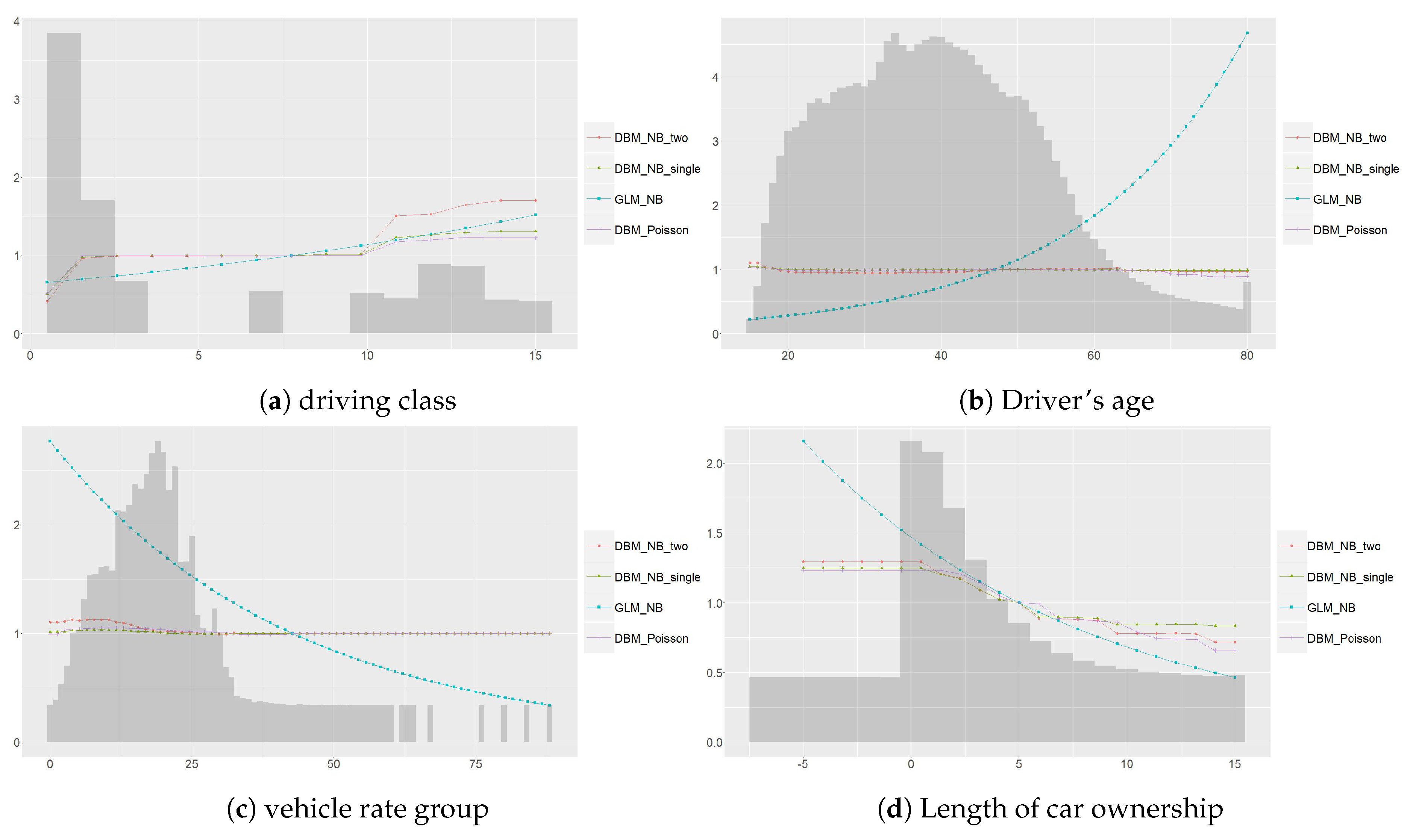
Partial dependence plot: actuaries can then dive further to understand the nuances about how individual variables predict differently through partial dependence plots. Defined in Friedman (2001), a partial dependence plot is a visualization that exhibits the marginal influence of F ( x ) on selected subsets of the input features. Similar to differential plots in actuarial practice, the plots can help actuaries to investigate the models in lower dimensions. For the case in negative binomial two-parameter regression, we are interested in the predicted response α β and thus we will study the partial dependence plot accordingly. As an illustration, the plots for driving class, driver’s age, years licensed, and the number of years with the insurers are depicted in Figure 3.
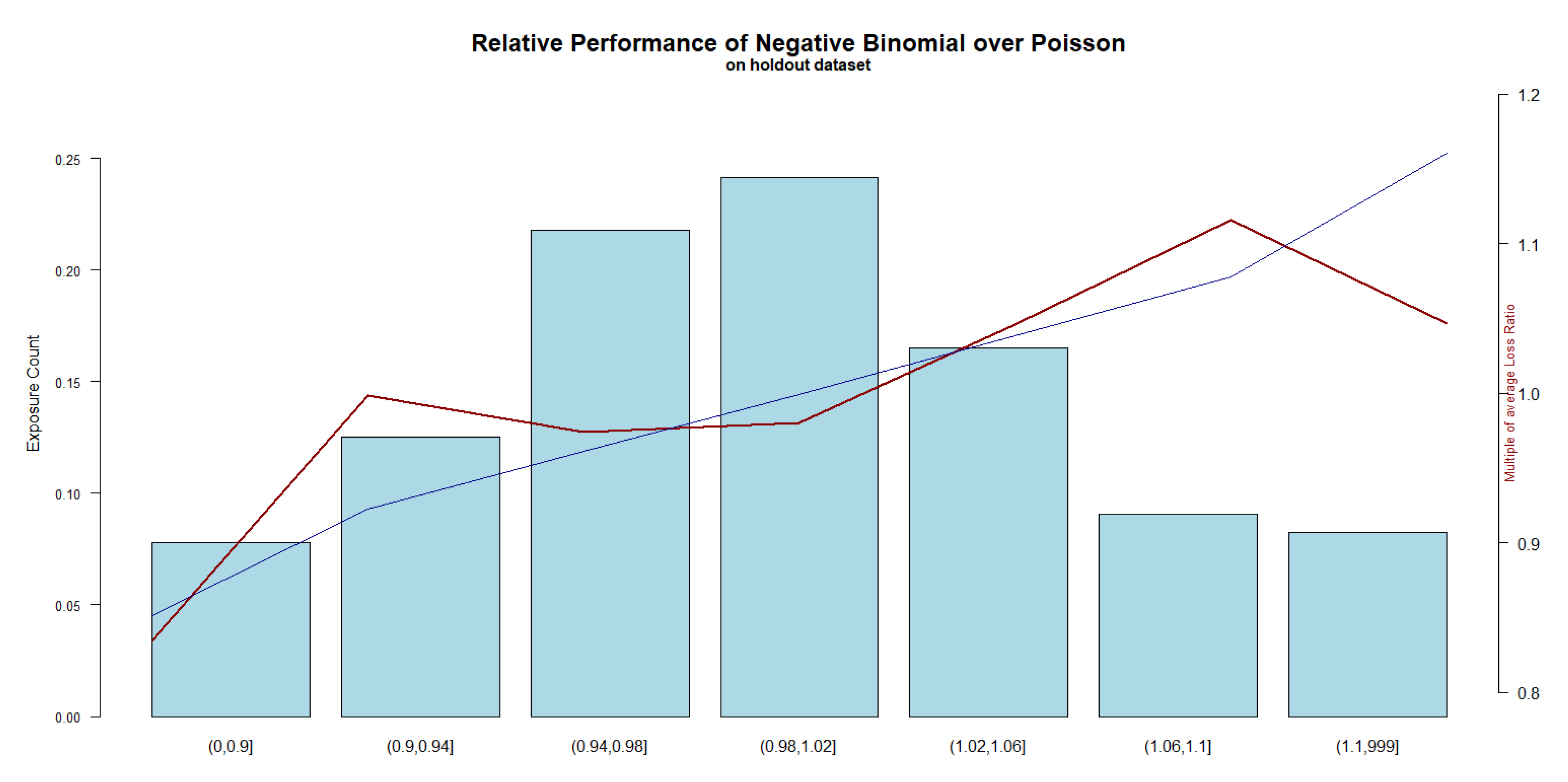
Double lift plot: the double lift plot provides a direct predictive performance comparison between the two-parameter negative binomial model over the Poisson model, both implemented through the DB. Observations are sorted in the ratios of the negative binomial prediction over the Poisson prediction and are grouped by the intervals that they belong (ratio of 0.99 ( 0.95 , 1 ] ). For each bucket, we calculate the ratio of actual claim counts over total Poisson prediction and ratio of total negative binomial prediction over total Poisson prediction. The red and blue lines describe the trend for the ratios respectively. Positively correlated lines indicate the negative binomial distribution explains a high portion of residuals that the Poisson model fails to capture. If no trend is observed, it indicates the ratio distributes randomly and thus the performance of both models is similar. On the contrary, a double lift plot with a negative trend would indicate the negative binomial is inferior to Poisson.
From actuarial perspectives, we can consider the negative binomial regression as a new costing algorithm, whereas the Poisson model as the current one. The ratio of the predictions by the new algorithm over the current prediction, called dislocation, is the rate change received by the insured. Correspondingly, the ratio of the total over the second is the loss ratio.
We explain the concept further through Figure 4. For insureds falling into the bucket with a low loss ratio, they should deserve a lower rate change. If the loss ratio is constant (no trend) or even negatively correlated with the dislocation, it indicates the new algorithm is not better. The dislocation exercise is an essential exercise for pricing actuaries as a rate increase will likely drive a high lapse rate whereas rate decrease may conceive profits. Thus, the rate change of both sides must be heavily studied and normally a rate capping is applied to temper extreme rate changes. With the double lift plot, actuaries have a viable tool to assess the accuracy of the new algorithm. Using the bucket of ( 0 , 0.9 ] as the example, the average dislocation (rate change) for this bucket is 0.85 (from the blue line) and the average loss ratio is 0.83 (red line), indicating that the proposed decrease reflects the risks inherited from the policyholders. Whereas, capping the rate increase for the bucket [ 1.1 , ) seems necessary as the rate increase is considerably higher than the indicated loss ratio.
From Figure 4, we witness a significantly positive relationship between the blue line (indicated rate change) and the red line (loss ratio), with a correlation of 0.82, indicating the negative binomial distribution is able to pick up the residuals from the Poisson’s.

7. Concluding Remarks and Directions of Future Research

This research aims to find an actuarial modeling approach to handle adeptly the over-dispersed insurance frequency data, price rigorously insurance products, and cut any untoward underwriting risks while following the principles of transparent systems for regulatory purposes, ease of the business interpretation. Retail insurance is a highly competitive domain and customers have a plethora of choices for comparing and picking among the most enthralling and economically viable insurances in the market. It implies that for insurers to compete healthily in the market, not only the pricing model has to be accurate in any coarse segments, but it also ought to be precise at the finer or individual levels. Otherwise, there will be an under-pricing risk, resulting in an operating loss whereas the loss incurred cannot be made up merely by over-pricing as some customers being over-priced will be driven away. In the study, a two-parameter estimation of negative binomial regression with specific consideration on the incomplete exposure, negative convexity and co-linearity has been able to handle the excessive zero data effectively and has presented a boosted predictive quality. Accurate forecasts can undoubtedly assist insurers to derive strategies that improve their overall competitiveness of the insurers along with hampering the exposure to the anti-selection problem, as compared with other competing candidates.
A few commonly used diagnostics are applied to evaluate the candidates. Efficacious use of the diagnostics can help the actuaries to thoroughly assess the applicability of predictive modeling techniques. We conclude this paper with a summary of insights observed in the empirical study:
  • Negative binomial regression performs better than the Poisson counterparts A meaningful improvement of metrics is observed with GLM, GAM, and DB, implementation of negative binomial as compared to the GLM, GAM and DB implementation of Poisson which clearly indicates that the negative binomial based models show a better fit for the insurance data, potentially due to the excessive zeros phenomenon described Section 1.
  • Existence of non-linearity and interaction In either Poisson or negative binomial based models, GAM outperforms GLM and DB outperforms GAM. The former suggests non-linearity between explanatory variables and the response where the later suggests that the existence of interaction within the data.
  • Two-parameter regression offers an additional boost of performance In this paper, we introduce a novel two-parameter regression approach through a simultaneous regression of both α and β . From the empirical study, assuming a fixed shape parameter may restrict the ability for a machine learning model to search for the best parameter set.
Incomplete exposure together with frequency estimation also impacts claim reserving. Claim reserves represent the insurer’s estimate of its current liabilities for unpaid claims that occurred on or prior to the financial statement reporting date (Friedland 2010). Hence, traditional statistics approach like expected claims, chain–ladder (CL), Bornhutter–Ferguson (CF), Cape Cod, Berquist–Sherman method are predominant. With the availability of modern machine learning techniques, actuaries are capable to estimate the liability at individual claim levels [Baudry and Robert (2019); Kuo (2019); Taylor (2019); Wüthrich (2018) and reference therein]. One significant contributing module of the early development of reserving is incurred but not yet reported, which can be effectively estimated by introducing a more realistic distribution assumption similar to the frequency modeling in our paper. In addition, the insights on incomplete exposure can possibly offer a meaningful actuarial research direction on proper handling in even more artificially split observation due to financial reporting purposes and thus leading to more robust estimates.

Funding

This research received no external funding.

Conflicts of Interest

The author declares no conflict of interest.

References

  1. Anderson, Duncan, Sholom Feldblum, Claudine Modlin, Doris Schirmacher, Ernesto Schirmacher, and Neeza Thandi. 2007. A Practitioner’s Guide to Generalized Linear Models—A Foundation for Theory, Interpretation and Application. CAS Discussion Paper Program. Arlington: Casualty Actuarial Society. [Google Scholar]
  2. Baudry, Maximilien, and Christian Y. Robert. 2019. A machine learning approach for individual claims reserving in insurance. Applied Stochastic Models in Business and Industry 35: 1127–55. [Google Scholar] [CrossRef]
  3. Boucher, Jean-Philippe, Michel Denuit, and Montserrat Guillen. 2009. Number of accidents or number of claims? an approach with zero-inflated poisson models for panel data. Journal of Risk and Insurance 76: 821–46. [Google Scholar] [CrossRef] [Green Version]
  4. Breslow, Norman. 1990. Tests of hypotheses in overdispersed poisson regression and other quasi-likelihood models. Journal of the American Statistical Association 85: 565–71. [Google Scholar] [CrossRef]
  5. Casualty Actuarial and Statistical Task Force. 2019. Regulatory Review of Predictive Models White Paper. Technical Report. Kansas City: National Association of Insurance Commissioners. [Google Scholar]
  6. Darroch, John N., and Douglas Ratcliff. 1972. Generalized iterative scaling for log-linear models. The Annals of Mathematical Statistics 43: 1470–80. [Google Scholar] [CrossRef]
  7. Dauphin, Yann N., Razvan Pascanu, Caglar Gulcehre, Kyunghyun Cho, Surya Ganguli, and Yoshua Bengio. 2014. Identifying and attacking the saddle point problem in high-dimensional non-convex optimization. In Advances in Neural Information Processing Systems. Montreal: Neural Information Processing Systems Conference, pp. 2933–41. [Google Scholar]
  8. David, Mihaela, and Dănuţ-Vasile Jemna. 2015. Modeling the frequency of auto insurance claims by means of poisson and negative binomial models. Annals of the Alexandru Ioan Cuza University-Economics 62: 151–68. [Google Scholar] [CrossRef] [Green Version]
  9. De Jong, Piet, and Gillian Z. Heller. 2008. Generalized Linear Models for Insurance Data. Cambridge: Cambridge University Press. [Google Scholar]
  10. Friedland, Jacqueline. 2010. Estimating Unpaid Claims Using Basic Techniques. Arlington: Casualty Actuarial Society, vol. 201. [Google Scholar]
  11. Friedman, Jerome H. 2001. Greedy function approximation: A gradient boosting machine. Annals of Statistics 29: 1189–232. [Google Scholar] [CrossRef]
  12. Gagnon, David R., Susan Doron-Lamarca, Margret Bell, Timothy J. O’ Farrell, and Casey T. Taft. 2008. Poisson regression for modeling count and frequency outcomes in trauma research. Journal of Traumatic Stress 21: 448–54. [Google Scholar] [CrossRef]
  13. Gini, Corrado. 1936. On the measure of concentration with special reference to income and statistics. Colorado College Publication, General Series 208: 73–79. [Google Scholar]
  14. Girosi, Federico, Michael Jones, and Tomaso Poggio. 1995. Regularization theory and neural networks architectures. Neural Computation 7: 219–69. [Google Scholar]
  15. Gourieroux, Christian, Alain Monfort, and Alain Trognon. 1984a. Pseudo maximum likelihood methods: Applications to poisson models. Econometrica: Journal of the Econometric Society 52: 701–20. [Google Scholar] [CrossRef]
  16. Gourieroux, Christian, Alain Monfort, and Alain Trognon. 1984b. Pseudo maximum likelihood methods: Theory. Econometrica: Journal of the Econometric Society 52: 681–700. [Google Scholar] [CrossRef]
  17. Haberman, Steven, and Arthur E. Renshaw. 1996. Generalized linear models and actuarial science. Journal of the Royal Statistical Society. Series D (The Statistician) 45: 407–36. [Google Scholar] [CrossRef]
  18. Hashem, Sherif. 1996. Effects of collinearity on combining neural networks. Connection Science 8: 315–36. [Google Scholar] [CrossRef]
  19. Henckaerts, Roel, Marie-Pier Côté, Katrien Antonio, and Roel Verbelen. 2019. Boosting insights in insurance tariff plans with tree-based machine learning. arXiv arXiv:1904.10890. [Google Scholar]
  20. Ismail, Noriszura, and Abdul Aziz Jemain. 2007. Handling overdispersion with negative binomial and generalized poisson regression models. Casualty Actuarial Society Forum 2007: 103–58. [Google Scholar]
  21. JO, Loyd-Smith. 2007. Maximum likelihood estimation of the negative binomial dispersion parameter for highly overdispersed data, with applications to infectious diseases. PLoS ONE 2: e180. [Google Scholar]
  22. Kingma, Diederik P., and Jimmy Ba. 2014. Adam: A method for stochastic optimization. arXiv arXiv:1412.6980. [Google Scholar]
  23. Kuo, Kevin. 2019. Deeptriangle: A deep learning approach to loss reserving. Risks 7: 97. [Google Scholar] [CrossRef] [Green Version]
  24. Lee, Simon, and Katrien Antonio. 2015. Why high dimensional modeling in actuarial science? Paper presented at the ASTIN, AFIR/ERM and IACA Colloquia, Sydney, Australia, August 23–27. [Google Scholar]
  25. Lee, Simon C. K., and Sheldon Lin. 2015. Delta boosting machine with application to general insurance. Paper presented at the ASTIN, AFIR/ERM and IACA Colloquia, Sydney, Australia, August 23–27. [Google Scholar]
  26. Lee, Simon CK, and Sheldon Lin. 2018. Delta boosting machine with application to general insurance. North American Actuarial Journal 22: 405–25. [Google Scholar] [CrossRef]
  27. Lim, Hwa Kyung, Wai Keung Li, and Philip L. H. Yu. 2014. Zero-inflated poisson regression mixture mode l. Computational Statistics and Data Analysis 71: 151–58. [Google Scholar] [CrossRef] [Green Version]
  28. Majumdar, Abhijit, Sayantan Chatterjee, Roshan Gupta, and Chandra Shekhar Rawat. 2019. Competing in a New Age of Insurance: How india Is Adopting Emerging Technologies. Technical Report. Chandigarh: PwC and Confederation of Indian Industry Northern Region. [Google Scholar]
  29. Naya, Hugo, Jorge I. Urioste, Yu-Mei Chang, Mariana Rodrigues-Motta, Roberto Kremer, and Daniel Gianola. 2008. A comparison between poisson and zero-inflated poisson regression models with an application to number of black spots in corriedale sheep. Genetics, Selection, Evolution: GSE 40: 379–94. [Google Scholar]
  30. Nelder, John Ashworth, and Robert W. M. Wedderburn. 1972. Generalized linear models. Journal of the Royal Statistical Society: Series A (General) 135: 370–84. [Google Scholar] [CrossRef]
  31. Ridout, Martin, Clarice G. B. Demetrio, Clarice, and John Hindle. 1998. Models for count data with many zeros. Paper presented at the International Biometric Conference, Cape Town, South Africa, December 14–18. [Google Scholar]
  32. Scollnik, David P. M. 2001. Actuarial modeling with mcmc and bugs. North American Actuarial Journal 5: 96–124. [Google Scholar] [CrossRef]
  33. Sun, Yanmin, Mohamed S. Kamel, Andrew K. C. Wong, and Yang Wang. 2007. Cost-sensitive boosting for classification of imbalanced data. Pattern Recognition 40: 3358–78. [Google Scholar] [CrossRef]
  34. Taylor, Greg. 2019. Loss reserving models: Granular and machine learning forms. Risks 7: 82. [Google Scholar] [CrossRef] [Green Version]
  35. Teugels, Jozef L., and Petra Vynckie. 1996. The structure distribution in a mixed poisson process. International Journal of Stochastic Analysis 9: 489–96. [Google Scholar] [CrossRef]
  36. Thomas, Janek, Andreas Mayr, Bernd Bischl, Matthias Schmid, Adam Smith, and Benjamin Hofner. 2018. Gradient boosting for distributional regression: Faster tuning and improved variable selection via noncyclical updates. Statistics and Computing 28: 673–87. [Google Scholar] [CrossRef] [Green Version]
  37. Tihonov, Andrei Nikolajevits. 1963. Solution of incorrectly formulated problems and the regularization method. Soviet Math. 4: 1035–38. [Google Scholar]
  38. Ver Hoef, Jay M., and Peter Boveng. 2007. Quasi-poisson vs. negative binomial regression: How should we model overdispersed count data? Ecology 88: 2766–72. [Google Scholar] [CrossRef] [PubMed] [Green Version]
  39. Werner, Geoff, and Claudine Modlin. 2010. Basic ratemaking. Casualty Actuarial Society 4: 1–320. [Google Scholar]
  40. Wüthrich, Mario V. 2018. Machine learning in individual claims reserving. Scandinavian Actuarial Journal 2018: 465–80. [Google Scholar] [CrossRef]
  41. Wuthrich, Mario V., and Christoph Buser. 2019. Data Analytics for Non-Life Insurance Pricing. Swiss Finance Institute Research Paper. Rochester: SSRN, pp. 16–68. [Google Scholar]
  42. Yang, Yi, Wei Qian, and Hui Zou. 2018. Insurance premium prediction via gradient tree-boosted tweedie compound poisson models. Journal of Business & Economic Statistics 36: 456–70. [Google Scholar]
  43. Yip, Karen CH, and Kelvin KW Yau. 2005. On modeling claim frequency data in general insurance with extra zeros. Insurance: Mathematics and Economics 36: 153–63. [Google Scholar] [CrossRef]
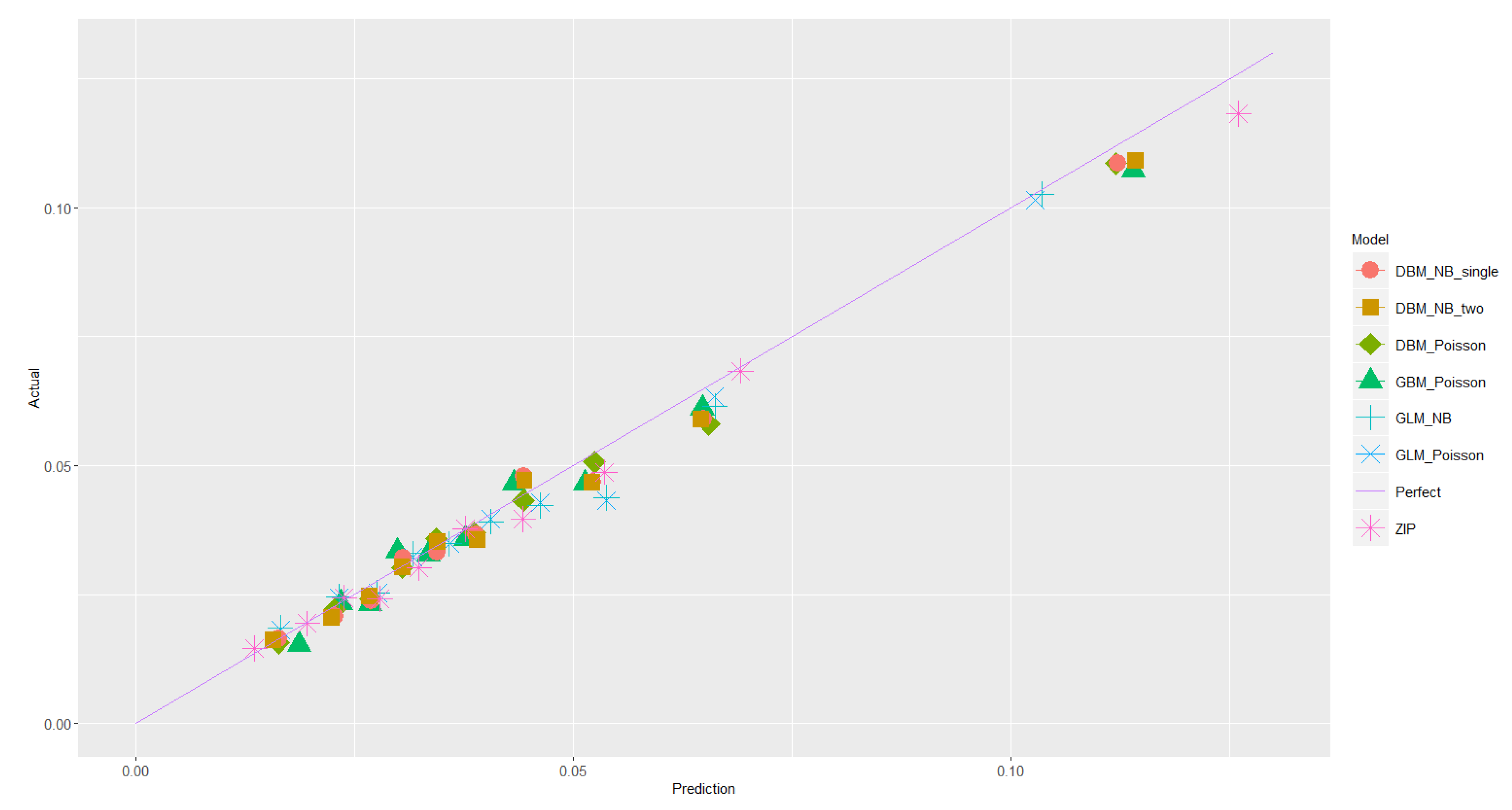
Figure 1. Lift plot for regression models.
Risks 08 00019 g001
Figure 2. Lorenz curve for candidate models.
Risks 08 00019 g002
Figure 3. Normalized marginal plots for modeling candidates.
Risks 08 00019 g003
Figure 4. Double lift plot for delta boosting (DB) implementation of negative binomial over Poisson.
Risks 08 00019 g004
Table 1. Key notation and definitions in this paper.
NotationDescription
MTotal number of observations for training
h ( x i ; a ) In decision tree, h ( · , · ) is a step function with a as the split point.
N j Index set of observation in Partition (can also be called Node or Leaf) j induced by h ( x i ; a )
G t ( x i ) = log ( α i , t ) α i , t as the shape parameter in the case of negative binomial regression.
F t ( x i ) = log ( β i , t ) β i , t as the scale parameter in the case of negative binomial regression.
Φ ( y i , F ¯ t ( x i ) ) The Loss function of observation i for DB regression. F t ( x i ) can be a vector of parameters. In negative binomial regression, the loss function is presented as Φ ( y i , G t ( x i ) , F t ( x i ) )
Φ ( y , F t ( x ) ) Aggregate loss function for one parameter regression, equivalent to i M Φ ( y i , F t ( x i ) )
Φ F , i , t and Φ G , i , t Φ F , i , t as an abbreviation of F t ( x i ) Φ ( y i , F t ( x i ) , G t ( x i ) ) . Similar for Φ G , i , t
Φ F F , i , t , Φ F G , i , t , Φ G G , i , t Φ G G , i , t as an abbreviation of 2 G 2 ( x i ) Φ ( y i , F t ( x i ) , G t ( x i ) ) . Similar for Φ F F , i , t and Φ F G , i , t
w i The exposure length of observation i
Φ F , i , t ( s , v ) The abbreviation of F t ( x i ) Φ ( y i , F t ( x i ) + s , G t ( x i ) + v ) , analogy for other first and second derivatives.
δ i Loss minimizer(delta) for observation i in the case of a single parameter estimation: δ i = argmin s Φ ( y i , l , ( F ^ t 1 ( x i ) + s ) )
Δ j Loss minimizer for observations in Node j: Δ j = argmin s i N j Φ ( y i , g 1 ( F ^ t 1 ( x i ) + s ) )
N L Partition that has a smaller A j in the case of a 2-node partition (Stunt)
N R Partition that has a larger A j in the case of a 2-node partition (Stunt)
Δ L Δ for observations in N L
Δ R Δ for observations in N R
Table 2. A simple illustration of the bookeeping in actuarial databases.
RecordyyyymmExposurePolicy IDAgeConvictionVehicle CodeClaimClaim $
12015010.0849 1 123456351CamrySE20130-
22015020.0767 2 123456351CamrySE20130-
32015030.0849 1 123456351CamrySE20130-
42015040.0274 1 123456351CamrySE20130-
52015040.0548 3 123456351LexusRX20150-
62015050.0411 1 123456351LexusRX20150-
72015060.0438 4 123456352LexusRX2015150,000.0
82015070.0849 1 123456352LexusRX20150-
92015080.0082 5 123456352LexusRX20150-
102015080.0767 6 123456362LexusRX20150-
1: Normal prorated accounting for the month. For example, the exposure for record 1 can be calculated as 0.849 = 31/365. 2: Regulation change with a new benefit schedule for minor accidents implemented. 3: Change of vehicle. 4: A claim is recorded. 5: Policy ends on August 3rd. 6: New term starts on August 4th.
Table 3. Models’ comparisons based on common diagnostic metrics.
ModelMetrics on Train DatasetMetrics on Test Dataset
Loss(P)Loss(NB)LiftGiniLoss(P)Loss(NB)LiftGini
GLM0.00-5.8070.2690.00-5.5750.245
GAM−277.36-6.7390.286−39.79-6.0090.312
GBM−764.80-8.9870.314−56.45-7.0220.292
Poissondbm−790.97 10.5200.317−63.88 6.9450.329
NBGLM−5.72−33.965.8260.2676.16−9.265.5270.256
NBGAM−264.75−288.396.7800.295−39.12−53.256.0870.259
NBdelta_single−782.02−528.8010.2850.322−61.45−68.606.5820.306
NBdelta_double−901.22−599.8110.3110.327−62.77−75.556.6940.332