Article

Application of Diffusion Models in the Analysis of Financial Markets: Evidence on Exchange Traded Funds in Europe

Faculty of Management and Economics, Gdansk University of Technology, Narutowicza 11/12, 80-233 Gdansk, Poland
*
Author to whom correspondence should be addressed.
Risks 2020, 8(1), 18; https://doi.org/10.3390/risks8010018
Submission received: 14 January 2020 / Revised: 7 February 2020 / Accepted: 10 February 2020 / Published: 14 February 2020
(This article belongs to the Special Issue Quantitative Methods in Economics and Finance)

Abstract

:
Exchange traded funds (ETFs) are financial innovations that may be considered as a part of the index financial instruments category, together with stock index derivatives. The aim of this paper is to explore the trajectories and formulates predictions regarding the spread of ETFs on the financial markets in six European countries. It demonstrates ETFs’ development trajectories with regard to stock index futures and options that may be considered as their substitutes, e.g., in risk management. In this paper, we use mathematical models of the diffusion of innovation that allow unveiling the evolutionary patterns of turnover of ETFs; the time span of the analysis is 2004–2015, i.e., the period of dynamic changes on the European ETF markets. Such an approach has so far rarely been applied in this field of research. Our findings indicate that the development of ETF markets has been strongest in Italy and France and weaker in the other countries, especially Poland and Hungary. The results highlight significant differences among European countries and prove that diffusion has not taken place in all the cases; there are also considerable differences in the predicted development paths.

1. Introduction

Over the last decades, dynamic changes across financial markets have included the introduction of innovative financial instruments that contribute to global financial diversity. The category of innovative financial instruments is highly heterogeneous, e.g., in terms of the rate of their expansion; exchange-traded funds (ETFs) are among the most rapidly expanding financial instruments. ETFs are funds structured to mimic the performance of selected financial assets, usually stock indexes. The difference between ETFs and conventional investment products (such as mutual funds) is that units of ETFs resemble, financial instruments such as listed equities or bonds because they are purchased and sold through stock exchanges. The growing popularity of ETFs, the increase in the sums involved and the rate of turnover are predominantly enhanced by low trading costs, low tracking errors, high liquidity and (in some countries) high tax efficiency (Agapova 2011; Madhavan 2016; Ben-David et al. 2017; Lettau and Madhavan 2018).
Until recently, ETFs were mainly considered as substitutes for index funds in passive investing strategies because of their similar features and users. However, a rising recognition and complexity of the products offered has resulted in increasing demand from different types of players in the financial markets. As a result, the shares of innovative funds have become substitutes not only for index funds but also for derivatives. To the best of our knowledge, there have been almost no empirical works covering the subject of switching between ETFs and stock index derivatives, although a theoretical background was provided by the framework suggested by Gastineau (2010). The only exception is the analysis of the Asia-Pacific markets presented in Marszk et al. (2019)—due to different geographical coverage, it cannot be compared directly to the current study. In the recent years, there have been a number of studies devoted to the relationships between ETFs and futures but they have focused on particular attributes of selected instruments rather than market-broad analysis (e.g., Liu and Tse 2017; Oztekin et al. 2017; Chang et al. 2018; Wang et al. 2018; Chang et al. 2019; Jiang et al. 2019; Wallace et al. 2019; Liu et al. 2020).
Even though the diffusion of financial innovations has been discussed in a number of publications in recent decades, most studies have focused on the banking sector (e.g., Persons and Warther 1997; Hayashi and Klee 2003; Frame and White 2004, 2012; Akhavein et al. 2005). Earlier studies of innovations in the capital markets mostly concentrated on asset-backed securities or junk bonds (see, e.g., McConnell and Schwartz 1992; Molyneux and Shamroukh 1996; DeMarzo and Duffie 1999). Since the global financial crisis, this category of research has been marginalized due to a decreasing popularity of these instruments (Philippas and Siriopoulos 2012). The studies that have considered the diffusion of innovative financial products traded on exchanges (such as ETFs) have been relatively rare (e.g., Lechman and Marszk 2015; Hull 2016; Marszk et al. 2019). However, the current analysis differs from the previous studies because we empirically examine the diffusion of ETFs in relation to the other stock index instruments in a highly heterogeneous group of countries in two regions. Some attempts to outline the theory of ETF adoption have also been made by Diaz-Rainey and Ibikunle (2012), Awrey (2013) and Blocher and Whaley (2016), but the process of diffusion has not been discussed in these publications.
According to data published by the ETF research company, ETFGI, the value of assets that are globally managed by ETFs reached a value of almost 4.7 trillion USD at the end of 2018, and there were circa 6500 such funds such funds available worldwide. In comparison, the global value of assets was 2.9 trillion USD at the end of 2015, and there were circa 6100 such funds; at the end of 2009 the corresponding figures were just over 1 trillion USD and fewer than 2000 ETFs. Nonetheless, in case of Europe, the substantial changes had taken place over 2004–2015, as it had been the period of the launch and rapid expansion of ETFs in terms of number, assets and turnover. However, the growth dynamics of the ETF markets (understood as increasing values of assets accompanied by an increased turnover rate) in different countries differed significantly. In Europe (here understood as the EU member countries; in other European countries, except for Switzerland, the ETF markets remain underdeveloped) their use is still low compared to other advanced economies such as the United States, Japan and South Korea. It is important to note that comparing most European ETF markets to their American or Far Eastern counterparts is problematic because ETFs have a longer history and wider recognition in these countries.
The main aim of this paper is to explore the trajectories and formulate forecasts regarding the spread of ETFs on the financial markets in selected European countries between 2004 and 2015: Germany, France, Spain, Italy, Poland and Hungary. Consequently, we exclusively analyze the EU member states: four countries with the most developed ETF markets in the examined time period (except for the United Kingdom, due to a lack of necessary data) and, for comparison, two countries in the Central and Eastern Europe with substantially underdeveloped ETF markets—we can thus examine radically different patterns of diffusion of ETFs. In order to reach the stated aim, we use a novel methodological approach to the analysis of financial markets—mathematical models of the diffusion of innovation based on the turnover data. We thus contribute to the present state of knowledge not only by addressing the role of ETFs among the index financial instruments in Europe, but also by showing the financial application of the diffusion models. Moreover, this is one of the first studies to present and examine ETFs and stock index derivatives as substitutes for risk management.
More specifically, we aim to:
  • analyze financial innovation diffusion trajectories across selected European stock exchanges;
  • provide long-term predictions of financial innovation development across the markets examined, in order to assess the probable path of ETF market development in Europe.
In order to do the above, we use monthly time series with ETF data from the economies selected between 2004 and 2015. This time period was selected due to the substantial pace of changes on the ETF markets in Europe, following their launch in the analyzed countries (the next years, since 2016 onwards, can generally be characterized as the period of stabilization and slower growth in terms of turnover of ETFs—moreover, in the case of some countries such as France or Spain, substantial decline could be noted; there were almost no ETFs traded in Europe prior to 2004).
This paper comprises five sections. Section 2 outlines the theoretical setting and presents some issues with regard to ETFs: their fundamentals, and how they compare with stock index derivatives. Section 3 outlines the methodological framework and presents the sources of data. Section 4 is devoted to the discussion of the results of the conducted empirical study; it is further divided into two parts: a presentation of introductory descriptive evidence related to the ETF market development, and a discussion of our key results obtained using diffusion models. Section 5 concludes the paper.

2. Theoretical Background

2.1. Basic Features of ETFs

In their basic form, exchange traded funds (ETFs) may be defined as baskets of securities (or other assets) traded on a stock exchange (comparable to equities of public corporations), typically with the intermediation of brokerage companies (Ferri 2009). ETFs are innovative financial instruments and they were introduced in the 1990s and 2000s. The units of ETFs closely replicate (i.e., track) the financial performance of certain financial assets, usually blue-chip or broad market indexes of the stock markets (Hehn 2005; Hill 2016). ETF shares (units) can be purchased and sold on the stock exchanges during their trading hours at prices determined by the interaction of demand and supply (Abner 2016; Investment Company Institute 2017). The prices of ETF shares remain typically at levels close to their net asset value (which is related to the prices of the assets tracked). There are two parts of the ETF market: the primary and secondary segments (Hill et al. 2015; Ben-David et al. 2018; Box et al. 2019). The shares of ETFs can be created and redeemed exclusively on the primary segment, as a result of operations including both the company that manages the fund (its sponsor) and financial institutions that act as authorized participants. In the case of physical ETFs, they involve the delivery of the assets underlying the fund in exchange for the shares of ETFs, and in the case of synthetic ETFs (the funds that employ derivatives, popular above all on the European markets) transactions involve cash. As a result of transactions on the primary market, which are a part of the arbitrage mechanism, ETF tracking errors (deviations in the returns on the units of ETFs from the returns on the tracked assets) are low in most cases. The secondary segment of the ETF market involves transactions on stock exchanges conducted by market participants (institutional or individual investors)—they include in particular the sale or purchase of ETF shares without any interaction with the managing company.
The rising recognition of ETFs in the last decade has generally been the result of the attributes they provide to investors compared to conventional financial instruments, particularly the sub-category of mutual funds with similar aims—index funds. These advantages stem from the mechanisms for the creation and distribution of ETFs. Their key benefits relative to index funds include: lower tracking errors and lower tracking costs (in some circumstances, index funds are more cost-efficient—this depends on the trading frequency and the investment period), higher liquidity (units of index funds are usually priced once a day and have daily buying/purchasing cycles) and greater tax efficiency in some countries (e.g., in the USA) (Agapova 2011; Investment Company Institute 2017; Piccotti 2018). It should not be forgotten that the expansion of ETFs in Europe can affect not only the financial sector but also non-financial companies—potential effects are not limited to the countries with the highest assets of locally listed ETFs, as other economies may also be affected through, e.g., cross-listing of the shares of ETFs (Alderighi 2020) or foreign assets held in the portfolios of ETFs (Baltussen et al. 2019); one of the possible consequences is the impact on the probability of bankruptcy of the companies (Kovacova et al. 2019) as the level of the development of the local ETF market can become one of the possible determinants of insolvency. However, this issue remains substantially understudied, both theoretically and empirically.

2.2. ETFs Compared to Stock Index Derivatives

Exchange traded funds, stock index futures and stock index options may be regarded as competing products within the category of (portfolio basket) index financial instruments. Together with a few other instruments, they constitute the equity index arbitrage complex—a group of related financial instruments based on common underlying assets (usually a basket of assets). This is a group of instruments with related values because of the similarity of their underlying financial assets (Gastineau 2010). The underlying assets are usually stock market indexes or stock baskets determined by the index rules. The equity index arbitrage complex consists of three instrument categories (less commonly used instruments have been omitted):
  • Traditional securities: baskets of equities and ETFs;
  • Symmetric derivatives: stock index futures and equity/index swaps;
  • (Non-symmetric) convex instruments: stock index options.
In this classification, ETFs are included in the first category because they are combinations and extensions of the underlying traditional assets, not because they lack innovative features. The values of symmetric instruments are straightforward functions of the prices of the underlying assets, whereas the prices of convex instruments do not move proportionately.
The following discussion regards three groups of instruments traded on exchanges: ETFs, stock index futures and stock index options. Stocks, the most basic instruments, are not discussed. Instruments which belong to an arbitrage complex are perceived by investors as substitutes, not only because of the similarity of the underlying assets but also because of the potential for (usually limited) arbitrage profits. This means that their prices are related. Treating the arbitrage complex as an object of analysis is a suitable way to perform research concerning modern financial markets, as feedback between increasing trading volumes and decreasing trading costs on the one hand and arbitrage complexes on the other has been observed on most of the world’s stock exchanges (Gastineau 2010).
Before the current dynamic development of the ETF market, these innovative instruments were considered as alternatives to futures or options, mostly for short- and long-term risk management by large investors. Gastineau (2010) presents the results of a preliminary comparison based on data from the US market (the assets tracked were S&P 500 stocks). The key characteristic compared is the cost of these two alternatives. The costs of ETFs for risk managers result from the cost of gathering the stocks in a creation basket (it is assumed that transactions are conducted on the primary ETF market due to their size) or opposite transactions—commission fees, management fees and market impact. In the case of futures, the main costs are roll risk (the cost of extending the contracts after they end) and market impact. As a result, futures seem to be a better choice for short-term risk management, whereas ETFs are beneficial in the long term due to their lack of rolling expenses.
In recent years, ETFs have become increasingly popular alternatives to futures and options, not only as risk management tools for specific categories of investors but also for a wider group of market participants. The reasons for this change in the financial landscape can be traced back to the financial crisis of 2008 and regulatory decisions made in its aftermath, which were aimed at reducing systematic shock risks (Goltz and Schröder 2011; Arnold and Lesné 2015). As a result of the increased cost of capital for investment banks, growing operational (e.g., improved transparency) and capital requirements, and liquidity constraints—mainly linked to the Basel III regulations (Madhavan et al. 2014; Madhavan 2016), the cost of traditional instruments such as futures or options grew and ETFs became relatively more cost-effective, for example in obtaining long-term exposure. Moreover, because of the high level of competition among ETF providers and economies of scale, the costs of investments in ETFs, especially in equity index ETFs (the closest substitutes for index futures and options), have been significantly declining (Arnold and Lesné 2015). To sum up, ETFs and stock index derivatives can be perceived as alternatives in certain fields of risk management (Hill and Mueller 2001; Madhavan 2016; Arunanondchai et al. 2019).
The differences between ETFs and stock index futures and in particular their relative advantages and disadvantages will now be described. Despite their different features, which make direct comparisons difficult, most of the relative advantages and disadvantages of futures with respect to ETFs which are discussed below also apply to options (as derivatives traded on regulated exchanges, which in many cases may be alternatives to futures, and even more importantly to ETFs (Thomsett 2016)).
The similarities between ETFs and stock index futures include (Goltz and Schröder 2011; Arnold and Lesné 2015; Marszk et al. 2019):
  • identical trading venues—most turnover occurs on stock exchanges,
  • multiple market participants,
  • intra-day pricing (on exchanges),
  • high liquidity,
  • minimal counterparty risk.
Table 1 presents some selected main features which distinguish ETFs from stock index futures. The key difference, which influences the relative costs of these two categories of instruments, lies in the rolling costs of futures contracts, i.e., the costs of entering a new contract after the expiry of the previous one, which involve both explicit costs (trading commissions and bid-ask spreads) and potential mispricing (Madhavan et al. 2014; Arnold and Lesné 2015). The main relative advantages of futures can be observed in the following features: the capital required, leverage, and short sale possibilities. The strengths of ETFs are higher accessibility, wider product ranges, minimal management requirements prior to exiting, no predefined maturity and easier foreign investment. To sum up, similarly to the use in risk management discussed in the preceding paragraphs, even for the broad investing audience, ETFs may be considered as more efficient long-term investment instruments, whereas futures are regarded as more suitable short-term choices (Eurex 2016). It should be noted, however, that the final choice depends not only on the holding period but also on the investment strategy. According to the results of a study conducted by the CME Group (2016), in the case of leveraged or short sale positions index futures are relatively more beneficial, regardless of the holding period.
It should be underlined that the framework presented above only applies to equity ETFs, and many more types of these instruments are currently available, such as fixed income and commodity ETFs. However, despite the increasing heterogeneity of ETFs, equity ETFs (based on the equity market, usually stock market indexes) are still by far the largest category.

3. Materials and Methods

3.1. Innovation Diffusion Models

To achieve the main aims of this study, we adopted a methodological framework allowing for examination of the evolution over time of the processes observed across the financial systems including, e.g., ETF diffusion. For that reason, apart from the usual descriptive statistics, we employed innovation diffusion models (presented in, inter alia, Geroski 2000; Rogers 2010; Lechman 2015); they may be used to approximate ETF diffusion trajectories and modeled projected future ETF development patterns. A similar approach is presented in a study by Lechman and Marszk (2015), who study ETF diffusion paths in chosen countries.
In the main part of our empirical analysis, in order to reveal ETF market development patterns, we follow the approach of, among others, Mansfield (1961) and Dosi and Nelson (1994), who adopted the concept of evolutionary dynamics. It can be expressed mathematically in the form of a logistic growth function, which may further be presented as an ordinary differential equation (Meyer et al. 1999):
dY x ( t ) dt = α Y x ( t ) .
If Y ( t ) denotes the level of variable x , α is a constant growth rate and t denotes time, then Equation (1) explains the time pattern of Y ( t ) . Moreover, the introduction of e to Equation (1) leads to its reformulation as:
Y x ( t ) = β e α t ,
or alternatively:
Y x ( t ) =   α exp β t ,
with notation parallel to the one in Equation (1) and β representing the starting level of x at t = 0 . Presented simple growth model is due to its assumptions being pre-defined as exponential. Therefore, it assumes that x will continue to grow infinitely in a geometric progression. Arbitrary extrapolation of Y x ( t ) within an exponential growth model can result in improbable predictions, since systems do not grow infinitely because of their constraints (Meyer 1994). For that reason, to address the issue of ‘infinite growth’, Equation (1) can be extended by adding a ‘resistance’ parameter (Kwasnicki 2013). This change imposes an upper ‘limit’ to the model, thus giving the original exponential growth curve a shape that is sigmoid. Consequently, the revised version of Equation (1) becomes a logistic differential function:
dY ( t ) dt = α Y ( t ) ( 1 Y ( t ) κ ) ,
with following notation—the parameter labeled as κ denotes the upper asymptote imposed, which arbitrarily restricts the increase of the variable Y .
As shown above, introducing a resistance parameter to exponential growth leads to trajectory that can be described as S-shaped. Equation (4), the 3-parameter logistic differential equation, can also be presented in another way, using a logistic growth function which takes non-negative values:
N x ( t ) = κ 1 +   e α t β ,
or, alternatively:
N x ( t ) = κ 1 + exp ( α ( t β ) ) ,
where N x ( t ) represents the level of variable x in certain time period t . Other parameters in Equations (5) and (6) stand for the following: κ is the upper asymptote, which determines the limit of growth and is also labeled ‘carrying capacity’ or ‘saturation’; α is the growth rate, which determines the speed of diffusion; and β stands for the midpoint, which shows the exact moment in time ( T m ) when the logistic pattern reaches 0.5 κ . Nonetheless, interpretation may be facilitated by replacing α with a parameter known as ‘specific duration’, and defined as Δ t = ln ( 81 ) α . With Δ t , it becomes easy to approximate the time necessary for x to increase from 10%κ to 90%κ. Moreover, the midpoint ( β ) denotes the point in time at which the logistic growth begins to level off. Finally, mathematically, it is the inflection point of the logistic curve. Incorporating Δ t and T m into Equation (6) produces:
N x ( t ) = κ 1 + exp [ ln ( 81 ) Δ t ( t T m ) ] .
In our research, we aim to use the methodological framework for innovation diffusion models briefly presented above. In the first part of the analysis, we assume that the growing value of ETF unit turnover can be regarded as diffusion of ETFs on financial markets in the examined countries. Nevertheless, in the core part of our study, we assume that the process of the growing ETF share of the total turnover of comparable investment options (in the equity index arbitrage complex) is comparable to the process of diffusion of innovative products and services across heterogeneous socio-economic systems. We assume that ETFs are innovations which due to a ‘word of mouth’ effect (Geroski 2000) and emerging network effects are progressively adopted by growing numbers of investors (who may also be described as ‘users’ of ETFs). We also rely on a basic assumption that investors (users) in certain type of financial innovations (here, ETFs) may freely contact ‘non-investors’ (‘non-users’), i.e., people either not using ETFs before or previously choosing other similar options, which leads to adoption by this group.
In short, we assume that ETFs diffuse on financial markets in the analyzed countries and gain a growing share of the total turnover of similar investment options (apart from ETFs, stock index futures and stock index options (Gastineau 2010; Madhavan 2016; Arunanondchai et al. 2019; Marszk et al. 2019)). In the fundamental specification of the 3-parameter logistic growth model as defined in Equation (6), we presume that N x ( t ) = ETF i ( t ) represents changes in the ETF share of the total turnover of comparable investment options over time t in country i. Put differently, it describes changes in country i`s level of ETF financial market penetration. The parameter κ is represented as κ i ETF , which is the ceiling (upper asymptote/system limit) on the process of ETF diffusion on financial markets. The estimated parameter κ i ETF denotes the potential ETF share of the total turnover of comparable investment options on the financial market in country i. However, there is the strict assumption that the trajectory of ETF diffusion (development) follows the sigmoid pattern generated by the logistic growth equation.
Next, the parameter α (as in Equation (6)) is represented as α i ETF , which is the speed of ETF diffusion on the financial market in country i. Hence, the estimated parameter α i ETF shows how fast the ETF share of the total turnover of comparable investment options is increasing on the financial market selected. Moreover, using parameter α i ETF we calculate the ‘specific duration,’ defined as Δ t = ln ( 81 ) α i ETF , which represents the time needed to pass from κ i ETF = 10 % to κ i ETF = 90 % .
The parameter β is expressed as β i ETF , and its estimated value denotes the midpoint Tm i ETF , which indicates the exact time when 50% of κ i ETF is reached. Hence, Tm i ETF represents the time (year/month) when the process of ETF diffusion reaches the half-way point if we assume that it is heading toward κ i ETF .
Thus, the modified specification of Equation (6) is:
ETF i ( t ) = κ i ETF 1 + exp ( α i ETF ( t β i ETF ) ) ,
with notation as explained above.
The parameters in Equation (8) can be estimated using not only ordinary least squares (OLS) but also maximum likelihood (MLE), algebraic estimation (AE) or nonlinear least squares (NLS). Nonetheless, as Satoh (2001) suggests, NLS returns the best predictions, as its estimates of standard errors (of κ i ETF , α i ETF , β i ETF ) are more valid than those returned using the other methods. Adopting NLS allows time-interval biases, which occur in the case of OLS estimates (Srinivasan and Mason 1986), to be avoided. However, NLS has the disadvantage that estimates of the parameters may be sensitive to the initial values of the time-series adopted. Finally, it should be emphasized that the construction of the utilized model hinders inclusion of the explanatory variables. However, the issue of the factors that affect the diffusion of ETFs was analyzed using different methodologies—the results were presented in, inter alia, Lechman and Marszk (2015) and Marszk et al. (2019).

3.2. Data

Our research covers stock exchanges in six European countries: two countries in the Central and Eastern Europe (CEE) region—Poland and Hungary; another four EU countries with the longest history of ETF trading—France, Italy, Germany and Spain. Our analysis covers the Euronext exchange considered as a whole (due to data availability), and thus (in addition to France) also includes The Netherlands, Belgium and Portugal. However, most of the turnover is reported to be in the French segment and so we decided to consider this exchange as if it was located in France. Consequently, we also used other indicators for France.
The time span of the analysis is 2004–2015. It was selected due to the high rate of changes on the ETF markets in Europe, following their launch in the analyzed countries. The beginning of this period was chosen due to the fact that there were almost no ETFs traded in Europe in 2003 or earlier. The selected end of the time period of analysis is 2015 as since 2016, the changes have been less significant. The time coverage is also a result of data availability. For the period 2004–2015 a balanced data set is available for most of the countries included in the analysis, while for the CEE countries, the time span of the analysis is shorter as ETFs were launched there later than in the advanced European economies.
The financial instrument databases used in the study are the dataset provided by the World Federation of Exchanges (World Federation of Exchanges 2017), datasets provided by the selected stock exchanges and reports published by these institutions. The most important financial indicators used are the turnover values (in USD millions) on the stock exchanges of the instruments selected: ETFs, stock index options and stock index futures. Monthly data are used.
Due to a lack of reliable data on the turnover of stock index futures and options on the main stock exchange in the United Kingdom (caused by changes in the organizational structure of the London Stock Exchange Group), it was excluded from the analysis.

4. Results

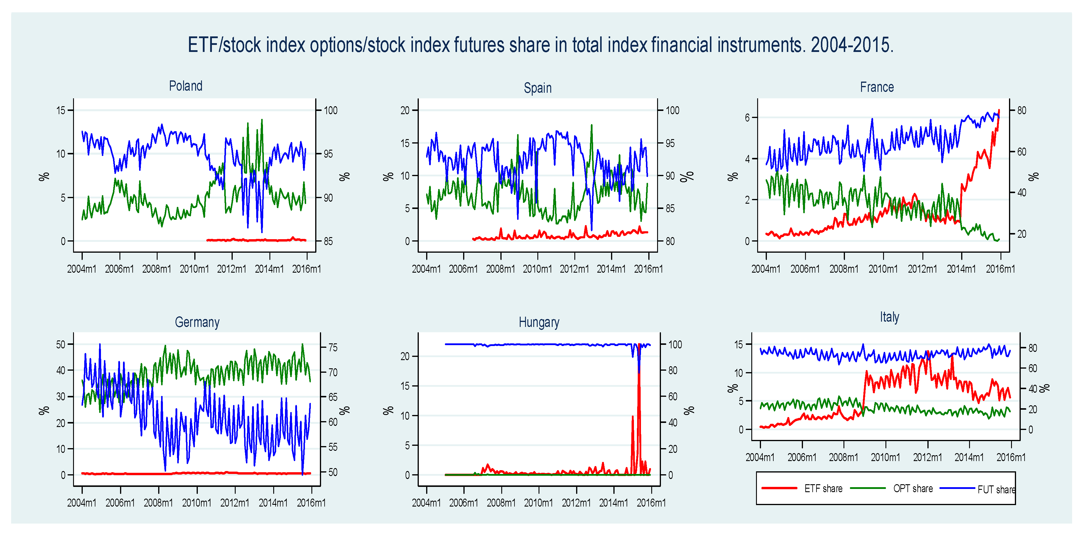
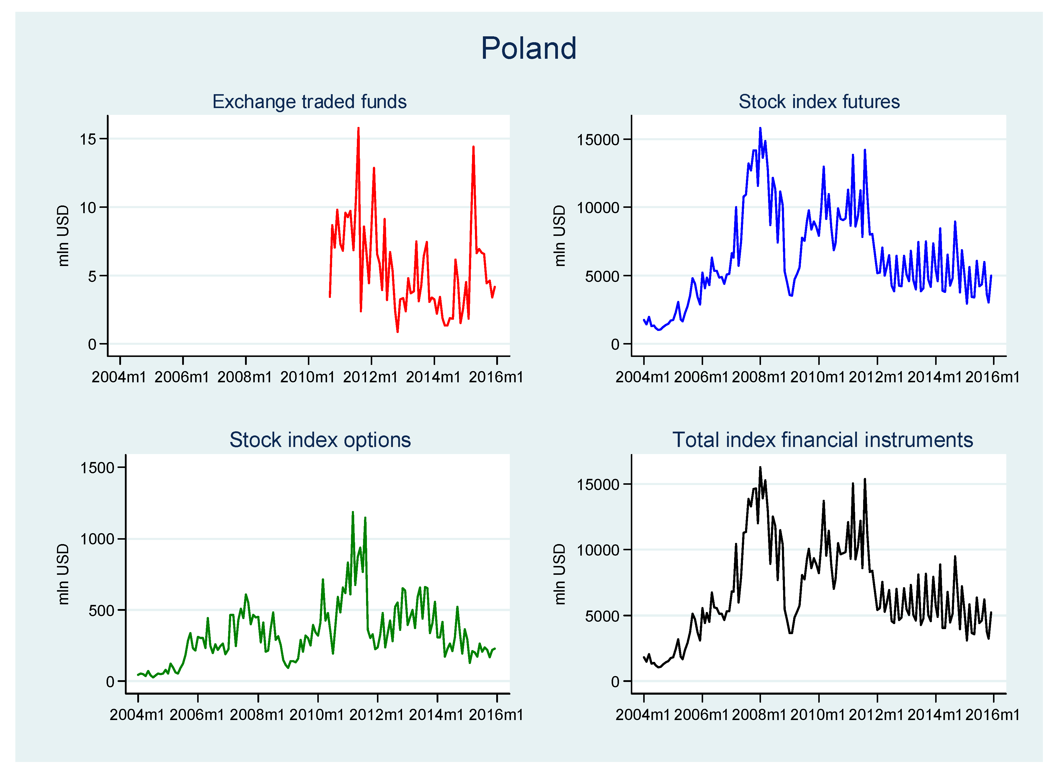
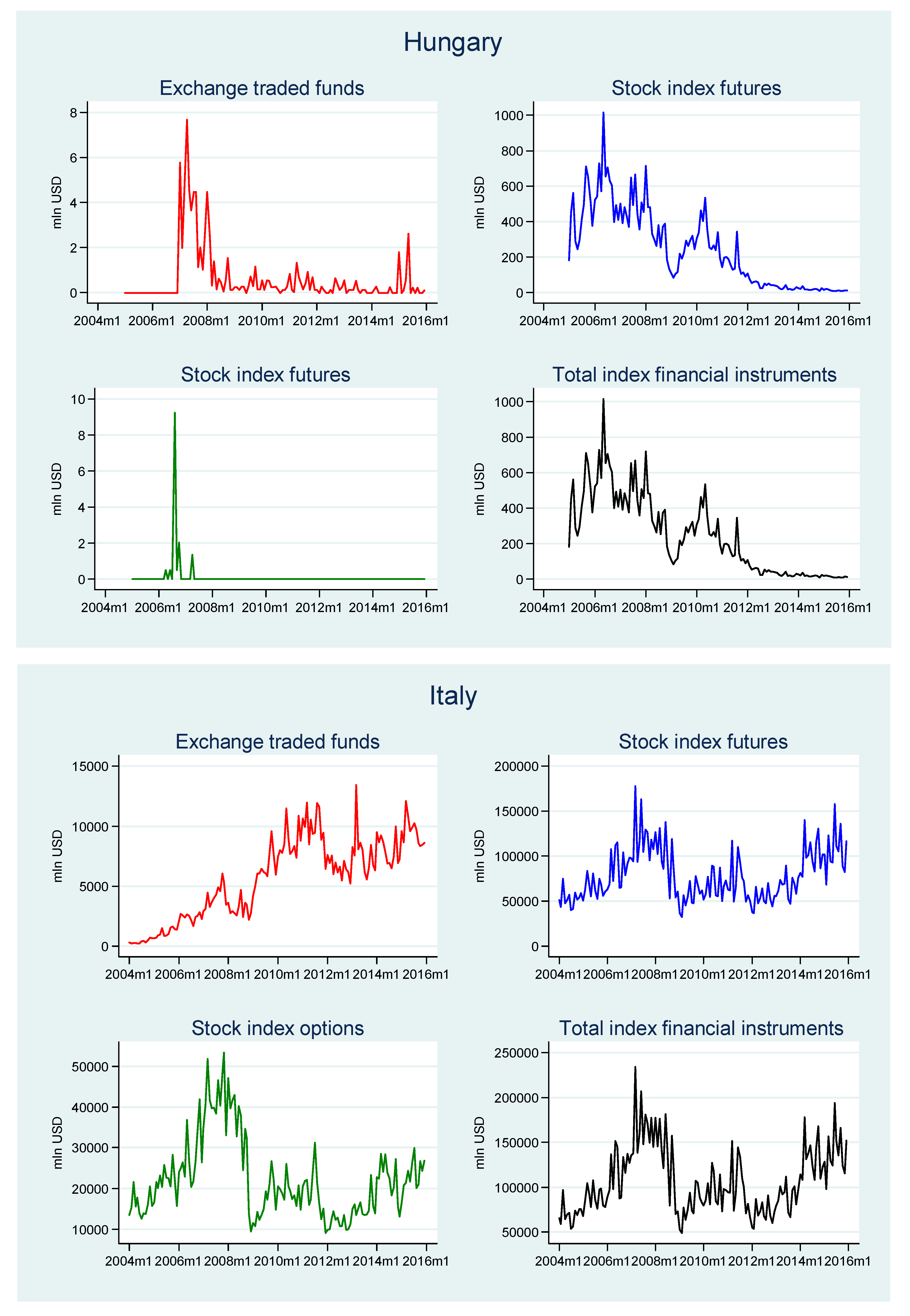
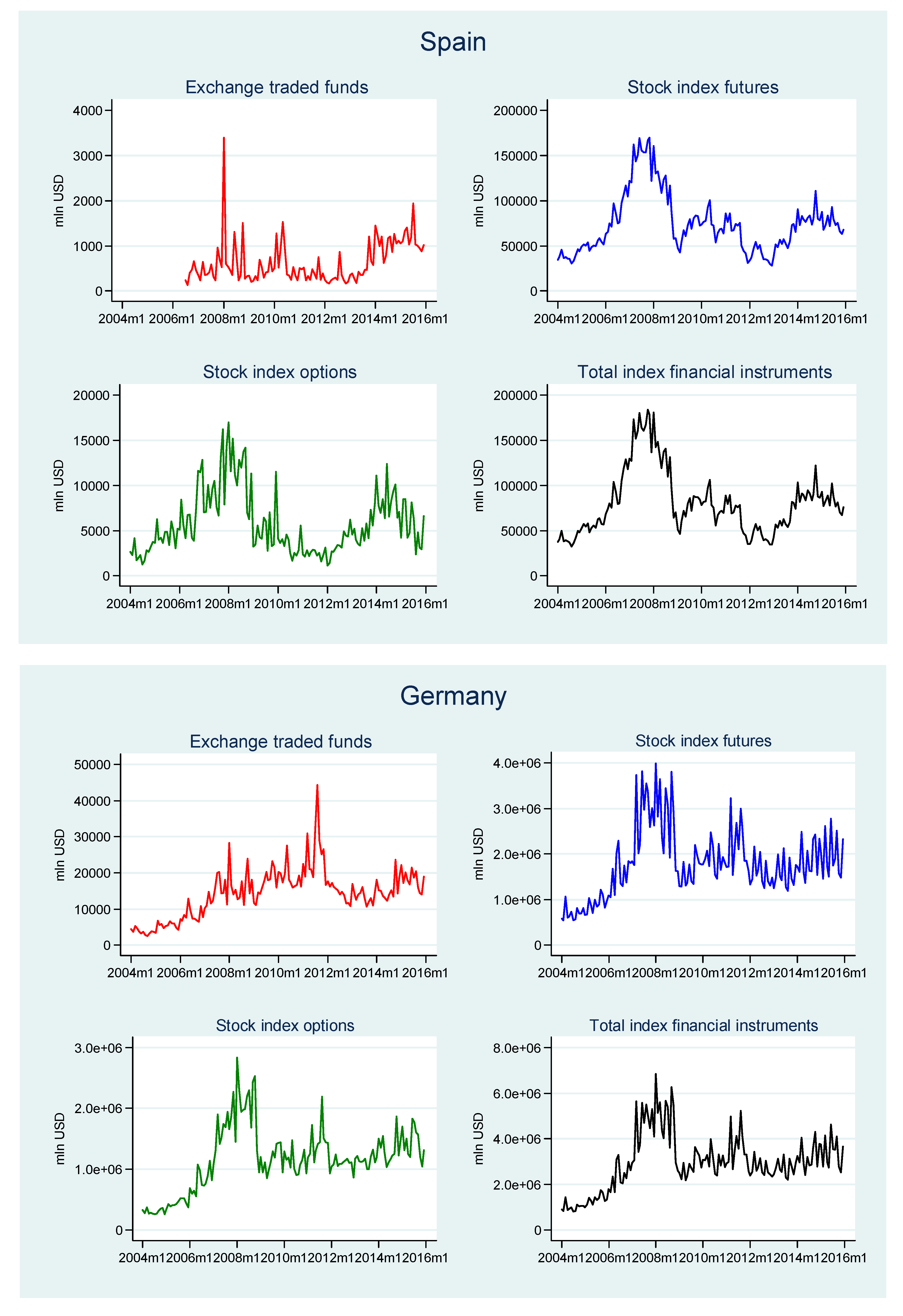
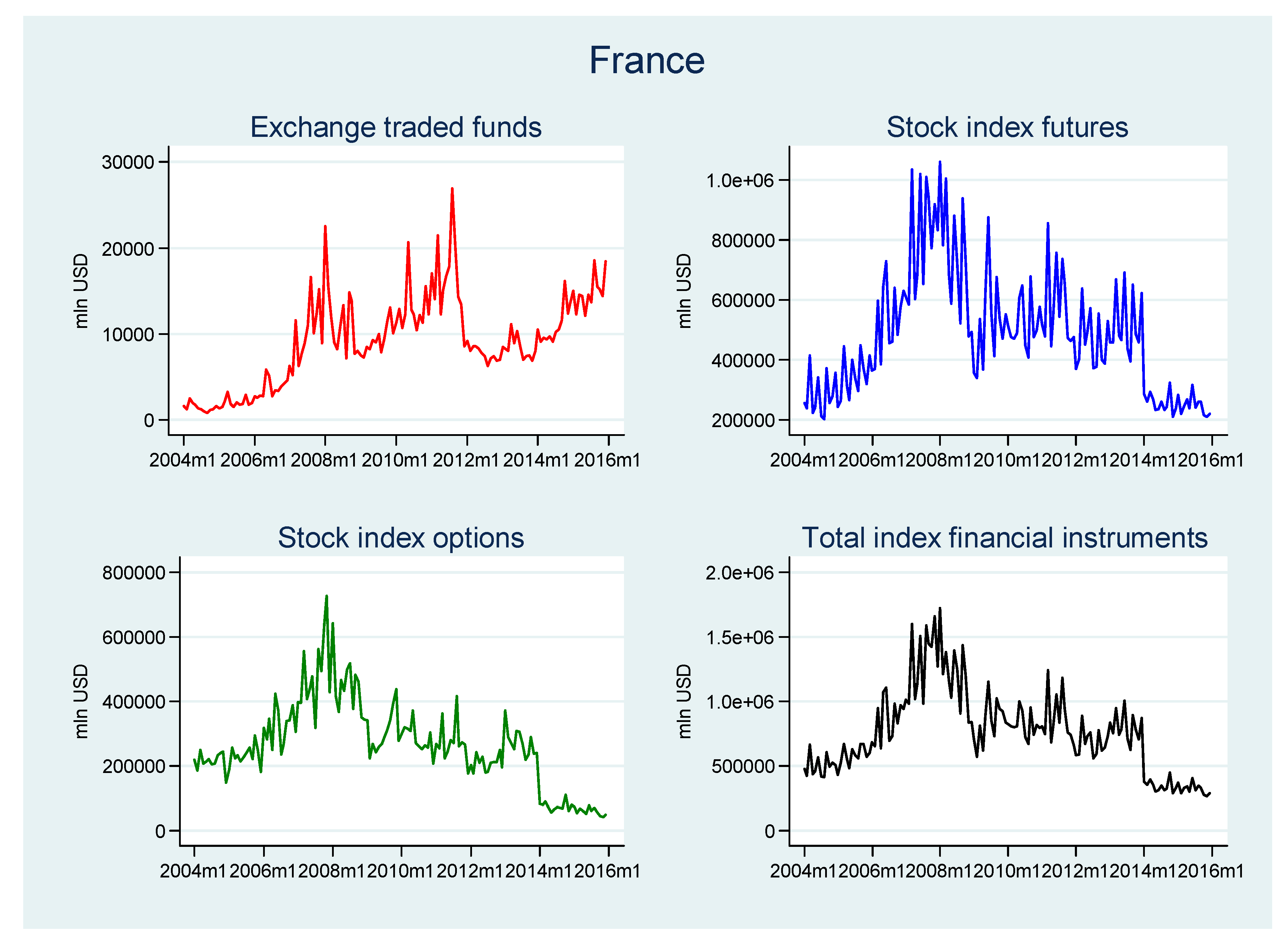
4.1. Exchange Traded Fund Market Development: Preliminary Evidence

Our investigation of the development of the ETF markets starts with an analysis of summary statistics on the key changes in two measures: the turnover value and the percentage share of the total turnover of index financial instruments (see Table 2).
In the time period analyzed, there were only two countries in the CEE region where ETFs were listed on the local stock exchanges: Poland and Hungary. In Poland, the highest values of ETF turnover were reached several months after their launch in September 2010, in August 2011 (see Table 2 and Figure A1 in the Appendix A). However, in 2012 turnover severely declined and reached a minimum level of only $0.9 million USD in November 2012. From 2013 to 2015, trading in ETFs was still at a rather low level. However, in April 2015, ETFs reached their maximum share of the total market: 0.39%, which was mostly caused by a one-month spike in ETF trading (yet it was still one of the lowest shares among the countries considered). In Hungary, ETFs were launched much earlier than in Poland (in 2007) but their turnover was significantly lower (a mean monthly value of $0.6 million USD compared to $5.5 million USD in Poland). As in Poland, the highest turnover values were observed soon after their introduction. However, in terms of ETF market share, the highest value in Hungary was reached (as in the Polish market) near the end of the time period analyzed, in May 2015 (see Figure 1). In contrast to the Polish exchange, the turnover of other related financial instruments (stock index futures and options) on the Hungarian market was extremely low: in most months there were almost no transactions in options and the value of futures trading was steadily declining. As a result, the mean turnover values in Hungary were minimal in comparison to the other stock exchanges considered. The very low turnover of ETFs in both Poland and Hungary was mostly caused by the low number of such financial products. In Poland, the number of ETFs grew from 1 to 3 (yet only one of them was listed exclusively in Poland and it accounted for the majority of turnover; the other two ETFs were cross-listed). In Hungary, there was only one ETF listed between 2007 and 2015 and it had a minimal turnover. The lack of further development was caused by a number of factors, including a lack of awareness of ETF features among market participants and the relatively small size of the financial markets, which limited the possibility of gaining benefits from the larger scale of offerings provided by ETF managers.
In the four advanced EU countries selected, the only country with no ETFs listed at the beginning of the time period analyzed was Spain (ETFs were launched in Spain in July 2006). In terms of ETF turnover, in Italy growth of the ETF market was somewhat stable and the highest values were reached near the end of the time period. In France and Germany, ETF turnover grew until 2011, when it sharply declined, which may be explained by the eurozone crisis and falling stock prices (in the other three advanced EU economies a decline in ETF turnover in 2011 was also observed but it was relatively weaker (see Figure A1 in the Appendix A)). After 2011, turnover in France began to grow, whereas in Germany it was stable. The Spanish ETF market developed in a different way. After much variability until 2011, it entered a stage of stability between 2012 and 2013, and from the end of 2013 it started growing. This shows that the development of the ETF markets in these countries was to some extent shaped by similar determinants (e.g., the euro-zone crisis), although there were also some country-specific factors despite the high level of financial market integration.
Regarding ETF market shares, some substantial differences between the four countries can be noticed (see Table 2 and Figure 1). In Spain and Germany, the market share of ETFs was very low over the whole period. The case of Germany is particularly interesting. The mean value of ETF turnover in this country was the highest among all the countries analyzed and one of the highest in the world. Nevertheless, their average market share was the second-lowest (it was only lower in Poland), which shows that the role of ETFs in Germany was negligible compared to that of other index financial instruments. In both France and Italy, the market share of ETFs increased considerably: in France particularly from 2014, and in Italy from 2009. The mean market share value of ETFs in Italy was the highest of all the countries under study (5.6%), yet was still much lower than the shares of the other index instruments. The rapid development of the Italian ETF market may to a large extent be explained by the acquisition of the Italian stock exchange by its British counterpart, which is one of the largest in Europe in terms of the number and turnover of ETFs. The two markets have been integrated in some areas, which considerably boosted the Italian stock exchange’s growth opportunities.
In the remainder of this study, we will use the market share as the indicator of ETF market development, as changes occurring in ETF markets should not be viewed in isolation but instead put in a broader context, thus showing the position of these innovative financial products in the financial system. Our preliminary analysis of changes occurring in the ETF markets will be expanded in the next sections—we will attempt to analyze the main features of the ETF diffusion process and predict its trajectories.

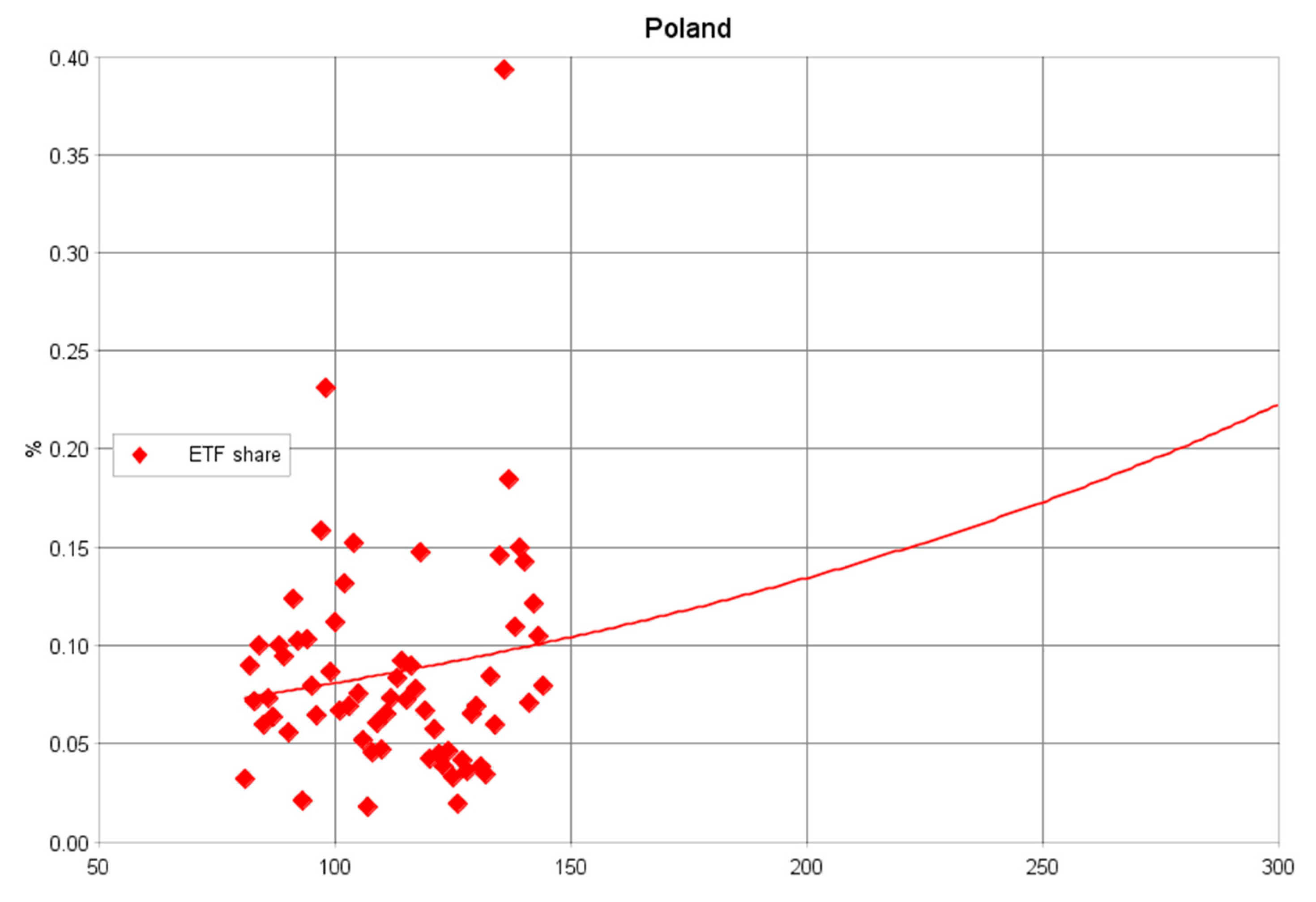
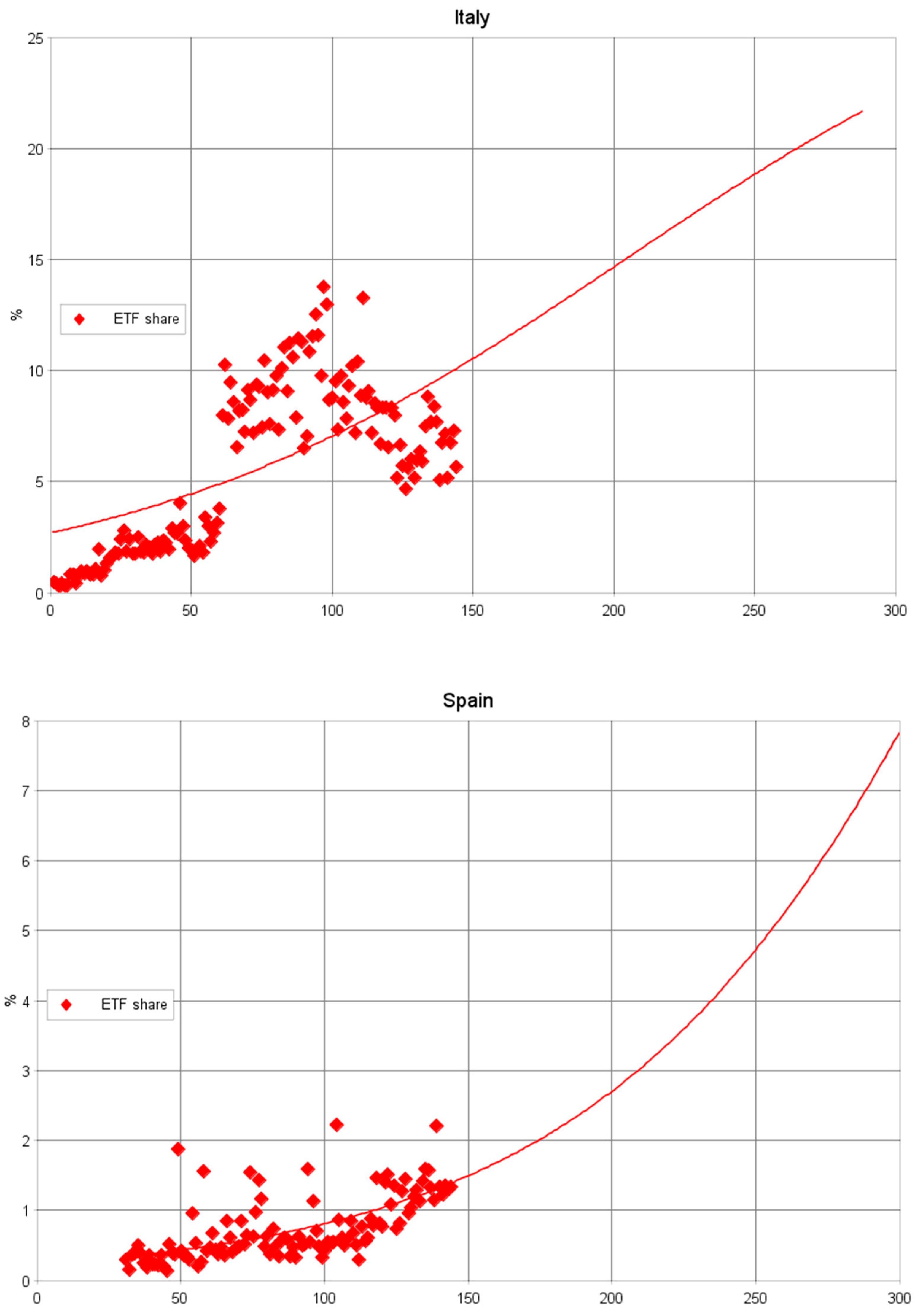
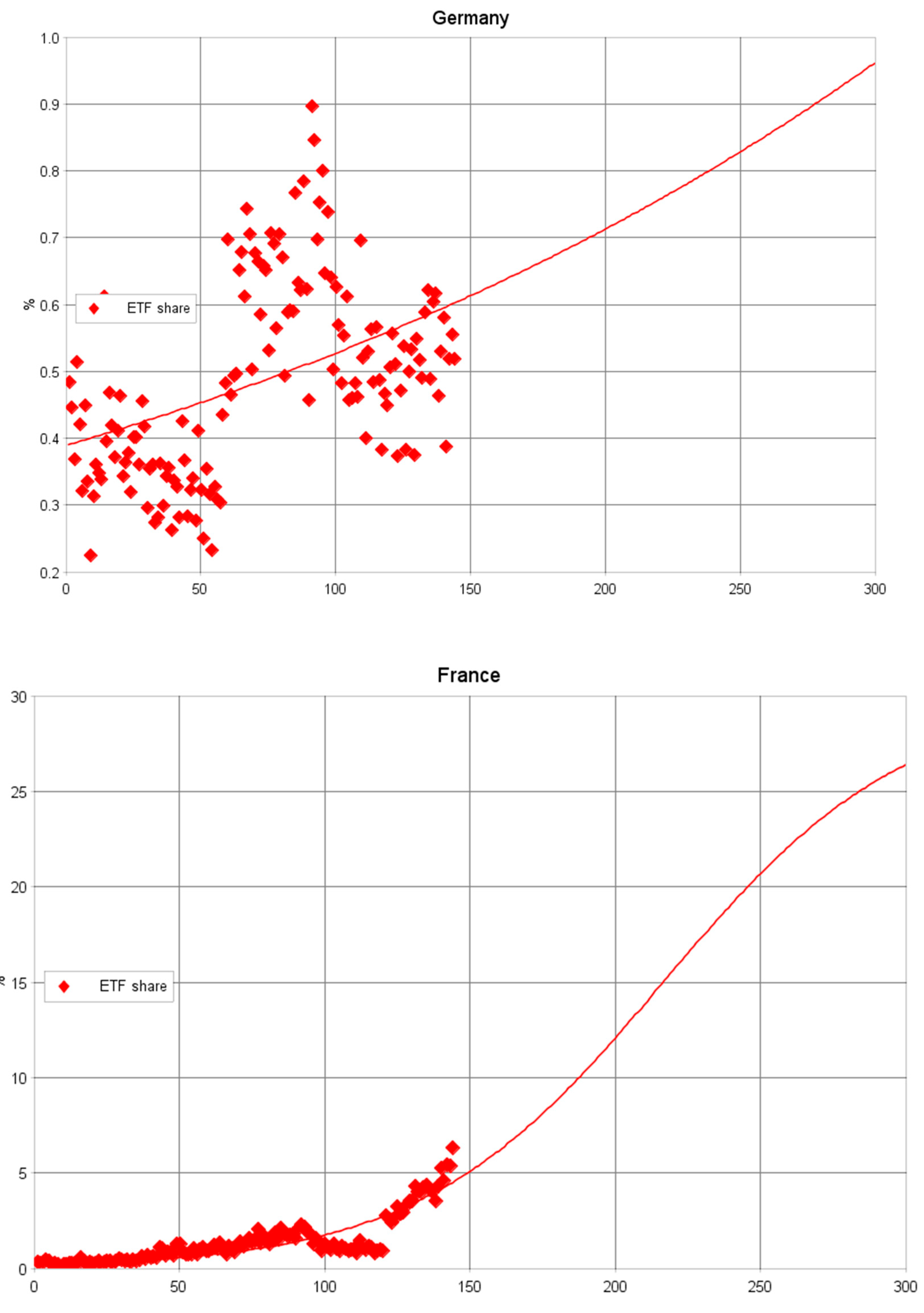
4.2. Exchange Traded Funds: Diffusion Models

As an aim of this study is to provide in-depth insight into the development process of ETFs across countries, we adopt a logistic growth model (for details, see Section 3) because use of this type of model allows the development trajectories of different variables in economic systems to be approximated and evaluated. Moreover, it allows the characteristic phases of the process of diffusion to be distinguished, such as the early diffusion phase, take-off, the exponential growth phase and saturation (maturity phase). Through the early diffusion stage, the number of contacts between adopters and non-adopters of a given innovation is still small, which may hinder its dissemination and so in this stage of diffusion the process is still reversible. However, under favorable conditions, easy contacts allow a domino effect to come into play and hence diffusion may speed up. Driven by various market forces, reductions in the cost of adopting innovations and multiple applications and uses of them, the number of new-users can rapidly increase and the curve takes off. It then enters a fast diffusion phase, when the diffusion process usually proceeds exponentially. Finally, a maturity (stabilization) stage is reached, during which the pace of diffusion again becomes slow and no substantial growth in the number of new users of the innovation is reported. In addition to revealing these phases, a simple logistic growth model returns good forecasts of future development (Kucharavy and De Guio 2011).
Following the above-mentioned approach and using monthly time series for the period 2004–2015, we develop logistic growth patterns and estimate parameters (see Section 3) representing the ETF share of total index financial instrument turnover for each country individually. The results of our analysis are presented in Figure A2 in the Appendix A, which shows that the current and predicted ETF share diffusion paths, and in Table 3, which summarizes the country-wise logistic growth model estimates.
The graphical evidence presented in Figure 1 suggests that ETF diffusion patterns in some countries (i.e., growing ETF shares) may be well described by the logistic (sigmoid) growth trajectory. In some cases, the characteristic phases of the S-shaped path can be distinguished (also see the analysis for other countries in Lechman and Marszk (2015)). Initially slow changes in the ETF share of total turnover of index financial instruments are followed by a sudden take-off and then the ETF share pattern enters the rapid growth phase. However, it is important to note that the shapes of the ETF share diffusion paths across the countries examined are different and so they need special attention.
The picture which emerges from analysis of the ETF share in the two selected CEE countries—Poland and Hungary—differs radically from that for other countries. As already mentioned in the previous section, in neither Poland nor Hungary did ETFs gain much popularity and their share of total turnover remained extremely low over the time period analyzed. In Hungary, the growth of the ETF share of total turnover was minimal and its role in shaping the financial market was negligible. In Poland, a diffusion of ETFs across the domestic financial market was reported but still their role and share of the total turnover was marginal. It should be noted that between 2004 and 2015, the ETF share of the total turnover was close to zero. This leads to the conclusion that in both Hungary and Poland a diffusion of ETFs did not take place and so logistic growth models should not be applied. Table 3 presents the estimates of logistic growth models for Poland and Hungary, but as in both cases the R2 of the models is zero, the parameters returned are misleading and inconclusive.
Finally, we discuss the results of the analysis of ETF diffusion for the four developed financial markets selected: Italy, Germany, France and Spain. In Germany, a diffusion of ETFs on the domestic financial market was not observed and ETF market penetration remained below 1%. As in the cases of Hungary and Poland, the logistic growth model estimates are not reliable. Despite the fact that the R2 of the model is 0.27 (see Table 3), the value returned for the midpoint (Tm) is negative and so cannot be treated as valid. The situation in Spain is analogous, with a very low ETF share of total turnover during the time period examined. At the end of 2015, Spain was still located in the early diffusion stage, and as a result reliable estimates of a logistic growth model are not possible (the logistic growth parameters returned cannot be treated as valid).
In the other two advanced European economies—France and Italy—the ETF share was relatively high between 2004 and 2015. In both cases, the ETF diffusion patterns take off into self-sustaining growth after the early diffusion stage, during which increases in the ETF share were slow. In the case of Italy, the specific take-off occurred relatively early compared to the other economies examined. It should be noted that between June and July 2008 the ETF share almost doubled (from 1.8% to 3.4%) and the take-off took place shortly afterwards—between the middle of December 2008 and January 2009, when the ETF share increased from 3.7% to 8.0%. All the parameters returned from the logistic growth model estimates for Italy are statistically significant. The R2 of the model is about 0.76, which implies a good fit between the empirical data and the theoretical model. Even though the R2 of the model is low, there are no obvious misspecifications as the diffusion of ETFs is relatively well described by the logistic growth trajectory. The upper asymptote is estimated as κ i ETF = 8.56%. The estimated midpoint is Tm i ETF = 52.9. The rate of diffusion is α i ETF = 0.113 and Δ t i ETF = 38.7, which can be interpreted as the number of months required to pass from 10% to 90% of κ i ETF .
For France too, the diffusion of ETFs is well described by the logistic growth trajectory, despite the fact that in this case the early diffusion stage was relatively long. The take-off into the exponential growth phase did not happen until between the middle of December 2013 and January 2014, when the ETF share of total turnover grew abruptly. Even though the diffusion of ETFs (in terms of market share) on the French financial market is well approximated by the logistic growth pattern, the parameters estimated for the logistic growth model are not valid. The upper asymptote (ceiling) is reported as κ i ETF = 7,755,333, which is a definite overestimation.
Regarding the process of ETF diffusion in our country sample, the eight economies can be divided into two groups. The first group encompasses two countries—France and Italy—where an early diffusion stage was followed by a take-off into an exponential growth phase along a sigmoid trajectory. These two countries managed to leave the early diffusion stage, during which ETF share growth was slow and spasmodic, and take off into rapid growth. In the other four countries, the ETF share did not leave the early diffusion stage and remained virtually locked at a low level.
This empirical analysis of ETF diffusion trajectories can be enriched by providing additional specifications of the predicted development of ETFs across the economies selected. Table 4 summarizes the predicted country-specific ETFs diffusion paths, and Figure A2 in the Appendix A portrays them graphically. Fixing the critical level of the upper asymptote ( κ i ETF ) at 5%, 7.5%, 10%, 15%, 20%, 25% and 30%, we predict logistic growth model parameters under the strict assumption that ETF market development will follow an S-shaped trajectory.
For Hungary, with κ i ETF fixed at 5% the predicted Tm i ETF is June 2027 and the ‘specific duration’ forecast is about 320 months, i.e., more than 26 years. The predicted rate of diffusion is 0.014, which implies that the speed of ETF diffusion will be rather low in Hungary. The forecasts for higher κ i ETF show even more distant midpoints and they cannot be treated as being very reliable (and also because of the low R2 of the models).
Italy has already reached the levels of κ i ETF = 5%, 7.5% and 10%. With κ i ETF fixed at 15%, the predicted Tm i ETF is April 2012 if the Italian ETF market follows an S-shaped trajectory. The predicted rate of diffusion is similar to that in Hungary, i.e., much lower than in, e.g., France.
Regarding Spain, with κ i ETF fixed at 5% the predicted Tm i ETF is July 2021 (considerably sooner than in the case of Hungary) and the ‘specific duration’ forecast is about 300 months. The rate of diffusion predicted is 0.015, which is consistent with the results obtained for Hungary and Italy. Finally, for France with κ i ETF fixed at 7.5%, the predicted Tm i ETF is July 2015 if the French ETF market follows the S-shaped trajectory. The rate of diffusion predicted for this level of κ i ETF is 0.028, but for higher levels it is slightly lower, which suggests that the diffusion of ETFs on the French market will be much faster than in other European countries.
The ETF diffusion paths predicted for Germany and Poland are not valid and so they will not be discussed. It should be emphasized that all these forecasts are tentative and should be treated with caution. The projected future diffusion paths are not entirely random but rather assume an S-shaped trajectory and all the predictions show a high level of sensitivity to historical data. Special caution is urged regarding the predictions referring to relatively high fixed ceilings like 20%, 25% and 30%, where the accuracy of the forecasts is questionable and they are to some extent misleading and inconclusive.

5. Conclusions

This extensive research was designed to analyze the development paths and dynamics of financial innovations introduced on stock exchanges in France, Germany, Spain, Italy—which have been treated as economies with relatively well developed stock exchanges—Hungary and Poland—two European economies where financial innovations have relatively short histories.
We examined the development of ETF markets using descriptive statistics and diffusion models. Graphical evidence on the ETF markets shows that ETF diffusion patterns in some countries may be described as a logistic growth trajectory—characteristic phases of the S-shaped path can be distinguished, which justifies the application of diffusion models. In Hungary and Poland, the level of ETF market development was very low and no significant changes are expected in the future unless the market environment is deeply transformed (which cannot be predicted). The trajectory of ETF market development in the more advanced European economies differed considerably. In Spain and Germany, the ETF market share remained very low and no meaningful predictions could be obtained using diffusion models. In France and Italy, significant development of ETF markets was identified and the predictions indicate potential further growth.
In our research we claimed that ETFs are financial innovations and thus it would be justifiable to analyze their development paths analogously to the process of diffusion of other tangible or intangible innovations. Following the latter, we have proposed to use the mathematical diffusion models, traditionally used to approximation of diffusion patterns of innovations, to draw the trajectories of ETFs diffusion across the financial markets. Our empirical evidence has demonstrated applicability of these diffusion models to the numerical analysis of ETFs diffusion process, allowing for detecting their in-time behavior, case-specific dynamics and development patterns, as well as providing long-term predictions. We believe that this approach to the analysis of financial markets development paves avenues for further and more profound research in this field (similar in-kind conclusions were reached in Marszk et al. (2019)).
Notably, ETFs as innovative financial instruments are still a poorly explored area, including our knowledge on what determines their development, or simply—what enhances or hinders their fast diffusion across financial markets. Apparently, in some countries, ETFs have rapidly gained popularity, while in other their development is negligible. The main limitation of the research method used in this study is that it is derived from the logistic growth function that is based on S-shaped trajectory of the diffusion of innovation which may be inconsistent with the attributes of the financial innovations. Moreover, our analysis has not addressed (with the exception of some preliminary suppositions) the factors that have influenced the diffusion processes. Detecting major determinants of ETFs diffusion in relation to other stock index instruments, including legal and institutional regulations that enable or stop this process, constitutes the direction of possible future research.

Author Contributions

Both authors contributed equally. Conceptualization, A.M. and E.L.; methodology, A.M. and E.L.; software, A.M. and E.L.; formal analysis, A.M. and E.L.; investigation, A.M. and E.L.; writing—original draft preparation, A.M. and E.L.; writing—review and editing, A.M. and E.L.; project administration, A.M. and E.L.; funding acquisition, A.M. and E.L. All authors have read and agreed to the published version of the manuscript.

Funding

This research was funded by project no. 2015/19/D/HS4/00399 financed by the National Science Centre, Poland. It was also supported by a grant from the CERGE-EI Foundation under a program of the Global Development Network.

Conflicts of Interest

The authors declare no conflict of interest. The funders had no role in the design of the study; in the collection, analyses, or interpretation of data; in the writing of the manuscript, or in the decision to publish the results.

Appendix A

Figure A1. ETFs, stock index options, stock index futures and total index financial instruments—diffusion trajectories. 2004–2015 (monthly time series). Values in USD millions.
Risks 08 00018 g0a1aRisks 08 00018 g0a1bRisks 08 00018 g0a1cRisks 08 00018 g0a1d
Figure A2. Current and predicted ETF diffusion patterns. Graphs and forecasts prepared using IIASA software.
Risks 08 00018 g0a2aRisks 08 00018 g0a2bRisks 08 00018 g0a2c

References

  1. Abner, David. 2016. The ETF Handbook. How to Value and Trade Exchange-Traded Funds, 2nd ed. Hoboken: John Wiley & Sons. [Google Scholar]
  2. Agapova, Anna. 2011. Conventional mutual index funds versus exchange-traded funds. Journal of Financial Markets 14: 323–43. [Google Scholar] [CrossRef]
  3. Akhavein, Jalal, W. Scott Frame, and Lawrence J. White. 2005. The diffusion of financial innovation: An examination of the adoption of small business credit scoring by large banking organizations. Journal of Business 78: 577–96. [Google Scholar] [CrossRef]
  4. Alderighi, Stefano. 2020. Cross-listing in the European ETP market. Economics Bulletin 40: 35–40. [Google Scholar]
  5. Arnold, Matthew, and Antoine Lesné. 2015. The Changing Landscape for Beta Replication—Comparing Futures and ETFs for Equity Index Exposure. Boston: State Street Global Advisors. [Google Scholar]
  6. Arunanondchai, Panit, Kunlapath Sukcharoen, and David J. Leatham. 2019. Dealing with tail risk in energy commodity markets: Futures contracts versus exchange-traded funds. Journal of Commodity Markets. [Google Scholar] [CrossRef]
  7. Awrey, Dan. 2013. Toward a supply-side theory of financial innovation. Journal of Comparative Economics 41: 401–19. [Google Scholar] [CrossRef]
  8. Baltussen, Guido, Sjoerd van Bekkum, and Zhi Da. 2019. Indexing and stock market serial dependence around the world. Journal of Financial Economics 132: 26–48. [Google Scholar] [CrossRef]
  9. Ben-David, Itzhak, Francesco Franzoni, and Rabih Moussawi. 2017. Exchange Traded Funds. Annual Review of Financial Economics 9: 169–19. [Google Scholar] [CrossRef]
  10. Ben-David, Itzhak, Francesco Franzoni, and Rabih Moussawi. 2018. Do ETFs increase volatility? The Journal of Finance 73: 2471–535. [Google Scholar] [CrossRef] [Green Version]
  11. Blocher, Jesse, and Robert E. Whaley. 2016. Two-Sided Markets in Asset Management: Exchange-traded Funds and Securities Lending. Vanderbilt Owen Graduate School of Management Research Paper 2474904: 1–45. [Google Scholar] [CrossRef]
  12. Box, Travis, Ryan L. Davis, and Kathleen P. Fuller. 2019. ETF competition and market quality. Financial Management 48: 873–916. [Google Scholar] [CrossRef]
  13. Chang, Chia-Lin, Chia-Ping Liu, and Michael McAleer. 2019. Volatility spillovers for spot, futures, and ETF prices in agriculture and energy. Energy Economics 81: 779–92. [Google Scholar] [CrossRef]
  14. Chang, Chia-Lin, Michael McAleer, and Chien-Hsun Wang. 2018. An econometric analysis of ETF and ETF futures in financial and energy markets using generated regressors. International Journal of Financial Studies 6: 2. [Google Scholar] [CrossRef] [Green Version]
  15. CME Group. 2016. The Big Picture: A Cost Comparison of Futures and ETFs. Chicago: CME Group. [Google Scholar]
  16. DeMarzo, Peter, and Darrell Duffie. 1999. A liquidity-based model of security design. Econometrica 67: 65–99. [Google Scholar] [CrossRef]
  17. Diaz-Rainey, Ivan, and Gbenga Ibikunle. 2012. A Taxonomy of the ‘Dark Side’ of Financial Innovation: The Cases of High Frequency Trading and Exchange Traded Funds. International Journal of Entrepreneurship and Innovation Management 16: 51–72. [Google Scholar] [CrossRef] [Green Version]
  18. Dosi, Giovanni, and Richard R. Nelson. 1994. An introduction to evolutionary theories in economics. Journal of Evolutionary Economics 4: 153–72. [Google Scholar] [CrossRef]
  19. Eurex. 2016. Futures or ETFs?—Not as Simple as Yes or No. Eschborn: Eurex. [Google Scholar]
  20. Ferri, Richard A. 2009. The ETF Book: All You Need to Know about Exchange-Traded Funds. Hoboken: John Wiley & Sons. [Google Scholar]
  21. Frame, W. Scott, and Lawrence J. White. 2004. Empirical Studies of Financial Innovation: Lots of Talk, Little Action? Journal of Economic Literature 42: 116–44. [Google Scholar] [CrossRef] [Green Version]
  22. Frame, W. Scott, and Lawrence J. White. 2012. Technological Change, Financial Innovation, and Diffusion in Banking. In The Oxford Handbook of Banking. Edited by Allen N. Berger, Philip Molyneux and John O.S. Wilson. Oxford: Oxford University Press, pp. 486–507. [Google Scholar] [CrossRef]
  23. Gastineau, Gary L. 2010. The Exchange-Traded Funds Manual. Hoboken: John Wiley & Sons. [Google Scholar]
  24. Geroski, Paul A. 2000. Models of technology diffusion. Research Policy 29: 603–25. [Google Scholar] [CrossRef]
  25. Goltz, Felix, and David Schröder. 2011. Passive Investing before and after the Crisis: Investors’ Views on Exchange-Traded Funds and Competing Index Products. Bankers, Markets and Investors 110: 5–20. [Google Scholar]
  26. Hamid, Nizam, and Jessica Edrosolan. 2009. A comparison: Futures, swaps, and ETFs. ETFs and Indexing 1: 39–49. [Google Scholar]
  27. Hayashi, Fumiko, and Elizabeth Klee. 2003. Technology adoption and consumer payments: Evidence from survey data. Review of Network Economics 2: 175–90. [Google Scholar] [CrossRef] [Green Version]
  28. Hehn, Elizabeth. 2005. Introduction. In Exchange Traded Funds: Structure, Regulation and Application of a New Fund Class. Edited by Elizabeth Hehn. Berlin/Heidelberg: Springer, pp. 1–5. [Google Scholar] [CrossRef]
  29. Hill, Joanne M. 2016. The evolution and success of index strategies in ETFs. Financial Analysts Journal 72: 8–13. [Google Scholar] [CrossRef]
  30. Hill, Joanne M., and Barbara Mueller. 2001. The appeal of ETFs. ETFs and Indexing 1: 50–65. [Google Scholar]
  31. Hill, Joanne M., Dave Nadig, and Matt Hougan. 2015. A Comprehensive Guide to Exchange-Traded Funds (ETFs). Charlottesville: CFA Institute Research Foundation. [Google Scholar]
  32. Hull, Isaiah. 2016. The development and spread of financial innovations. Quantitative Economics 7: 613–36. [Google Scholar] [CrossRef] [Green Version]
  33. Investment Company Institute. 2017. Investment Company Fact Book 2017. Washington, DC: Investment Company Institute. [Google Scholar]
  34. Jiang, Tao, Si Bao, and Long Li. 2019. The linear and nonlinear lead–lag relationship among three SSE 50 Index markets: The index futures, 50ETF spot and options markets. Physica A: Statistical Mechanics and its Applications 525: 878–93. [Google Scholar] [CrossRef]
  35. Kovacova, Maria, Tomas Kliestik, Katarina Valaskova, Pavol Durana, and Zuzana Juhaszova. 2019. Systematic review of variables applied in bankruptcy prediction models of Visegrad group countries. Oeconomia Copernicana 10: 743–72. [Google Scholar] [CrossRef] [Green Version]
  36. Kucharavy, Dmitry, and Roland De Guio. 2011. Logistic substitution model and technological forecasting. Procedia Engineering 9: 402–16. [Google Scholar] [CrossRef] [Green Version]
  37. Kwasnicki, Witold. 2013. Logistic growth of the global economy and competitiveness of nations. Technological Forecasting and Social Change 80: 50–76. [Google Scholar] [CrossRef]
  38. Lechman, Ewa, and Adam Marszk. 2015. ICT technologies and financial innovations: The case of Exchange Traded Funds in Brazil, Japan, Mexico, South Korea and the United States. Technological Forecasting and Social Change 99: 355–76. [Google Scholar] [CrossRef] [Green Version]
  39. Lechman, Ewa. 2015. ICT Diffusion in Developing Countries: Towards a New Concept of Technological Takeoff. New York: Springer. [Google Scholar] [CrossRef]
  40. Lettau, Martin, and Ananth Madhavan. 2018. Exchange-Traded Funds 101 for Economists. Journal of Economic Perspectives 32: 135–54. [Google Scholar] [CrossRef] [Green Version]
  41. Liu, Pan, Dmitry Vedenov, and Gabriel J. Power. 2020. Commodity financialization and sector ETFs: Evidence from crude oil futures. Research in International Business and Finance 51: 101109. [Google Scholar] [CrossRef]
  42. Liu, Qingfu, and Yiuman Tse. 2017. Overnight returns of stock indexes: Evidence from ETFs and futures. International Review of Economics & Finance 48: 440–51. [Google Scholar] [CrossRef]
  43. Madhavan, Ananth, Ursula Marchioni, Wei Li, and Daphne Yan Du. 2014. Equity ETFs versus Index Futures: A Comparison for Fully Funded Investors. Institutional Investor Journal 5: 66–75. [Google Scholar] [CrossRef]
  44. Madhavan, Ananth. 2016. Exchange-Traded Funds and the New Dynamics of Investing. Oxford: Oxford University Press. [Google Scholar] [CrossRef]
  45. Mansfield, Edwin. 1961. Technical change and the rate of imitation. Econometrica: Journal of the Econometric Society 29: 741–66. [Google Scholar] [CrossRef] [Green Version]
  46. Marszk, Adam, Ewa Lechman, and Yasuyuki Kato. 2019. The Emergence of ETFs in Asia-Pacificirca. New York: Springer. [Google Scholar] [CrossRef]
  47. McConnell, John J., and Eduardo S. Schwartz. 1992. The origin of LYONS: A case study in financial innovation. Journal of Applied Corporate Finance 4: 40–47. [Google Scholar] [CrossRef]
  48. Meyer, Perrin S., Jason W. Yung, and Jesse H. Ausubel. 1999. A primer on logistic growth and substitution: The mathematics of the Loglet Lab software. Technological Forecasting and Social Change 61: 247–71. [Google Scholar] [CrossRef]
  49. Meyer, Perrin. 1994. Bi-logistic growth. Technological Forecasting and Social Change 47: 89–102. [Google Scholar] [CrossRef]
  50. Molyneux, Phil, and Nidal Shamroukh. 1996. Diffusion of Financial Innovations: The Case of Junk Bonds and Note Issuance Facilities. Journal of Money, Credit and Banking 28: 502–22. [Google Scholar] [CrossRef]
  51. Oztekin, A. Senol, Suchismita Mishra, Pankaj K. Jain, Robert T. Daigler, Sascha Strobl, and Richard D. Holowczak. 2017. Price discovery and liquidity characteristics for US electronic futures and ETF markets. The Journal of Trading 12: 59–72. [Google Scholar] [CrossRef] [Green Version]
  52. Persons, John C., and Vincent A. Warther. 1997. Boom and bust patterns in the adoption of financial innovations. Review of Financial Studies 10: 939–67. [Google Scholar] [CrossRef]
  53. Philippas, Dionisis Th, and Costas Siriopoulos. 2012. Is the progress of financial innovations a continuous spiral process? Investment Management and Financial Innovations 9: 20–31. [Google Scholar] [CrossRef]
  54. Piccotti, Louis R. 2018. ETF Premiums and Liquidity Segmentation. Financial Review 53: 117–52. [Google Scholar] [CrossRef]
  55. Rogers, Everett M. 2010. Diffusion of Innovations, 4th ed. New York: Free Press. [Google Scholar]
  56. Satoh, Daisuke. 2001. A discrete bass model and its parameter estimation. Journal of the Operations Research Society of Japan-Keiei Kagaku 44: 1–18. [Google Scholar] [CrossRef] [Green Version]
  57. Srinivasan, V., and Charlotte H. Mason. 1986. Technical note—nonlinear least squares estimation of new product diffusion models. Marketing Science 5: 169–78. [Google Scholar] [CrossRef]
  58. Thomsett, Michael. 2016. Differences Between Stock and Future Options. InvestorGuide.com. Available online: http://www.investorguide.com/article/12605/differences-between-stock-and-future-options-wo/ (accessed on 13 February 2020).
  59. Wallace, Damien, Petko S. Kalev, and Guanhua Lian. 2019. The evolution of price discovery in us equity and derivatives markets. Journal of Futures Markets 39: 1122–36. [Google Scholar] [CrossRef]
  60. Wang, Jinzhong, Hao Kang, Fei Xia, and Guowei Li. 2018. Examining the equilibrium relationship between the Shanghai 50 stock index futures and the Shanghai 50 ETF options markets. Emerging Markets Finance and Trade 54: 2557–76. [Google Scholar] [CrossRef]
  61. World Federation of Exchanges. 2017. WFE Database. London: World Federation of Exchanges. [Google Scholar]
Figure 1. ETFs, stock index options and stock index futures—share of total turnover of index financial instruments. 2004–2015 (monthly time series). Left-hand Y axis—ETF share of total index financial instruments; right-hand Y axis—stock index options and stock index futures share of total index financial instruments.
Risks 08 00018 g001
Table 1. Main differences between ETFs and stock index futures. Own compilation based on Hamid and Edrosolan (2009), Madhavan et al. (2014), Arnold and Lesné (2015), CME Group (2016), Madhavan (2016), Arunanondchai et al. (2019), Marszk et al. (2019).
FeatureETFsStock Index Futures
AccessibilityVery high, due to small notional requirements. Operationally simple in most casesSmall notional requirements. Operationally complicated (e.g., pricing)
Product rangeVery broad. Many asset classesMost major equity indexes
Required capitalFull upfront paymentOnly margin (a notional fraction of the investment needs to be posted)
Position managementMinimal (may include reinvestment of dividends)Margin and cash flow management, contract rolling
MaturityOpen-endedPredefined (usually one or three months)
LeverageOnly in the case of leveraged ETFsAvailable, usually very high
Short sales of securitiesMay be limited (with the exception of special ETF classes, e.g., inverse ETFs)Investors may use futures to obtain short exposure
Positions in foreign assetsNo need to manage foreign exchange componentForeign exchange management necessary
Table 2. Summary statistics for exchange traded funds, stock index options, stock index futures and total index financial instruments. Monthly data for 2004–2015. For ETFs, the periods of analysis are: Poland, 2010m9–2015m12; Hungary, 2007m1–2015m12; Italy, 2004m1–2015m12; Spain, 2006m7–2015m12; Germany, 2004m1–2015m12; and France, 2004m1–2015m12. The number of ETFs varies across time periods and countries.
StatisticsPolandHungary
Turnover on Local Stock Exchanges (in million USD)
ETFsStock Index OptionsStock Index FuturesTotal Index Financial InstrumentsETFsStock Index OptionsStock Index FuturesTotal Index Financial Instruments
# obs.64144144144132132132132
Min0.9029.141041.051070.20.00.09.210.08
(2012m11)(2004m7)(2004m7)(2004m7) (2015m5)(2015m7)
Max15.791187.115,820.616,274.57.69.21015.61015.6
(2011m8)(2011m3)(2008m1)(2008m1)(2007m4)(2006m8)(2006m5)(2006m5)
Mean5.5336.26422.66761.300.600.10244.9245.7
Absolute change in value (pp)0.76184.053220.63408.8−5.60.0−172.7−0.25
Average monthly dynamic100.3101.1100.7100.748.666.897.997.9
Share of Total Turnover of Index Financial Instruments on Local Stock Exchanges [%]
ETFsStock Index OptionsStock Index Futures-ETFsStock Index OptionsStock Index Futures-
# obs.64144144-132132132-
Min0.021.686.010.00.077.9-
(2012m11)(2008m4)(2008m4) (multiple periods)(multiple periods)(2015m)
Max0.3913.998.422.011.4100-
(2015m4)(2013m8)(2013m8) (2015m5)(2006m8)(multiple periods)
Mean0.085.0594.9-0.550.0299.4-
Absolute change in share (pp)0.051.9−2.00-−0.250.0−0.89-
Average monthly dynamic101.4100.499.9-39.760.799.9-
ItalySpain
Turnover on Local Stock Exchanges (in million USD)
ETFsStock Index OptionsStock Index FuturesTotal Index Financial InstrumentsETFsStock Index OptionsStock Index FuturesTotal Index Financial Instruments
# obs.144144144144114144144144
Min246.49038.9932,881.448,685.7131.21134.128,439.732,317.4
(2004m5)(2011m12)(2009m2)(2009m2)(2012m8)(2012m1)(2012m2)(2004m8)
Max13,435.253,337.8178,067.9234,279.73397.516,971.7169,693.3183,875.7
(2015m3)(2007m3)(2007m3)(2007m3)(2008m1)(2008m1)(2007m11)(2007m10)
Mean5669.722,329.078,508.4106,507.1630.55764.674,557.780,821.5
Absolute change in value (pp)8306.913,222.264,909.386,438.5779.13950.733,361.538,333.1
Average monthly dynamic102.3100.5100.6100.6101.3100.6100.4100.5
Share in Total Turnover of Index Financial Instruments on Local Stock Exchanges [%]
ETFsStock Index OptionsStock Index Futures-ETFsStock Index OptionsStock Index Futures-
# obs.144144144 114144144-
Min0.2710.763.6 0.1481.681.6-
(2004m3)(2014m12)(2007m10) (2007m9)(2011m1)(2012m12)
Max13.732.383.3 2.296.896.8-
(2012m1)(2007m10)(2014m12) (2015m7)(2012m12)(2011m1)
Mean5.620.973.4 0.757.192.3-
Absolute change in share (pp)5.2−3.07−2.1 1.041.6−2.9-
Average monthly dynamic101.799.899.9 101.3100.199.9-
GermanyFrance
Turnover on Local Stock Exchanges (in million USD)
ETFsStock Index OptionsStock Index FuturesTotal Index Financial InstrumentsETFsStock Index OptionsStock Index FuturesTotal Index Financial Instruments
# obs.144144144144144144144144
Min2549.1259,180.4550,142.9823,511.8810.644,421.9204,785.8269,320.8
(2004m9)(2004m12)(2004m2)(2004m7)(2004m9)(2015m11)(2004m8)(2015m11)
Max44,323.22,830,9183,993,3536,852,53126,980.5726,885.41,059,8431,725,926
(2011m8)(2008m1)(2008m1)(2008m1)(2011m8)(2007m11)(2008m1)(2008m1)
Mean14,351.31,161,1631,781,5252,957,0409170.3266,211.7485,718.8761,100.9
Absolute change in value (pp)14,556.7979,971.11,747,9452,742,47316,803.99−168,972−33,997.2−186,165
Average monthly dynamic101.0100.9100.9100.9101.798.999.999.6
Share of Total Turnover of Index Financial Instruments on Local Stock Exchanges [%]
ETFsStock Index OptionsStock Index Futures-ETFsStock Index OptionsStock Index Futures-
# obs.144144144-144144144-
Min0.2224.0649.40.1316.549.5-
(2004m9)(2004m12)(2015m7) (2004m9)(2015m11)(2004m8)
Max0.8950.0675.66.450.378.7-
(2011m7)(2015m7)(2004m12) (2015m12)(2004m8)(2015m5)
Mean0.4838.660.9-1.433.964.5-
Absolute change in share (pp)0.03−0.310.27-6.00−28.722.7-
Average monthly dynamic100.099.9100.0-102.099.3100.2-
Table 3. Diffusion of exchange traded funds (as share of total turnover of index financial instruments). Logistic growth model estimates. 2004–2015 (monthly time series). Poland—data from 2010m9; Hungary—data from 2005m1; Spain—data from 2006m7.
ParameterPolandHungaryItaly
κ i ETF (ceiling/upper asymptote)0.08797,2078.56
Tm i ETF ( β i ETF ) (midpoint)397,133.9106252.9
α i ETF (rate of diffusion)−2606.70.0130.113
Δ t i ETF (specific duration)−0.002339.238.7
R2 of the model0.000.0750.76
# of obs. 64130 (outliers excluded)144
ParameterSpainGermanyFrance
κ i ETF (ceiling/upper asymptote)500,100.20.5857,755,333.6
Tm i ETF ( β i ETF ) (midpoint)1,175,6.2−3.94777.3
α i ETF (rate of diffusion)0.0120.0260.023
Δ t i ETF (specific duration)354.4169.8194.2
R2 of the model0.4110.270.789
# of obs. 114144144
Table 4. Predicted ETFs diffusion patterns (as share of total turnover of index financial instruments). Hungary—outliers excluded. Italics = misspecifications.
κ i E T F (Upper Asymptote)—Fixed T m i E T F (Midpoint)—Refers to a Specific Date Δ t i E T F (Specific Duration)—Number of Months α i E T F (Rate of Diffusion) R2 of the Model
Poland
5%229,626,799249,867,8960.000.016
7.5%981.7857.40.0050.018
10%1,010.6859.50.0050.018
15%258,875,673220,949,4930.000.016
20%1,181,1862.70.0050.018
25%1,225.8863.30.0050.018
30%1,262.3863.80.0050.018
Hungary
5%282.4 (2027m6)319.50.0140.073
7.5%318.3 (2030m6)326.00.0130.073
10%343.2 (2032m7)329.30.0130.073
15%377.4 (2035m5)332.60.0130.074
20%401.2 (2037m5)334.20.0130.074
25%419.4 (2038m11)335.20.0130.074
30%434.2 (2040m2)335.90.0130.074
Italy
5%Already achieved
7.5%Already achieved
10%Already achieved
15%100.24 (2012m4)246.90.0180.485
20%141.7 (2015m9)318.70.0140.454
25%175.7 (2018m7)359.90.0120.445
30%204.1 (2020m12)386.90.0110.435
Spain
5%211.4 (2021m7)300.30.0150.41
7.5%252.4 (2024m12)318.20.0140.41
10%280.6 (2027m4)327.20.0130.41
15%318.9 (2030m6)336.30.0130.41
20%345.4 (2032m9)340.80.0130.41
25%365.6 (2034m5)343.50.0130.41
30%381.7 (2035m9)345.40.0130.41
Germany
5%1,402.61426.90.0030.02
7.5%892.61349.10.0030.02
10%1003.81375.00.0030.02
15%1156.01401.00.0030.02
20%1261.31413.90.0030.02
25%1341.71421.70.0030.02
30%730.81297.30.0030.02
France
5%Already achieved
7.5%139.9 (2015m7)157.60.0280.73
10%156.8 (2016m12)165.60.0270.75
15%179.7 (2018m11)174.50.0250.76
20%195.3 (2020m3)179.20.0250.77
25%207.2 (2021m3)182.10.0240.77
30%216.6 (2021m12)184.00.0240.77

