A Likelihood Approach to Bornhuetter–Ferguson Analysis

Abstract

A new Bornhuetter–Ferguson method is suggested herein. This is a variant of the traditional chain ladder method. The actuary can adjust the relative ultimates using externally estimated relative ultimates. These correspond to linear constraints on the Poisson likelihood underpinning the chain ladder method. Adjusted cash flow estimates were obtained as constrained maximum likelihood estimates. The statistical derivation of the new method is provided in the generalised linear model framework. A related approach in the literature, combining unconstrained and constrained maximum likelihood estimates, is presented in the same framework and compared theoretically. A data illustration is described using a motor portfolio from a Greek insurer.

1. Introduction

While high dimensional data and its validation is important for many machine learning experiments, it is also true that many machine learning applications combine mathematical statistical methods with prior knowledge. The difficulty is to include this prior knowledge to upgrade the statistical analysis without violating the fundamental principles of mathematical statistics. These kinds of applications are omnipresent in insurance reserving, which often cite the original paper of Bornhuetter and Ferguson from 1972. This combination of prior knowledge and mathematical statistics is the purpose of this paper, where we are able to make it while sticking to the classical maximum likelihood technique of mathematical statistics.

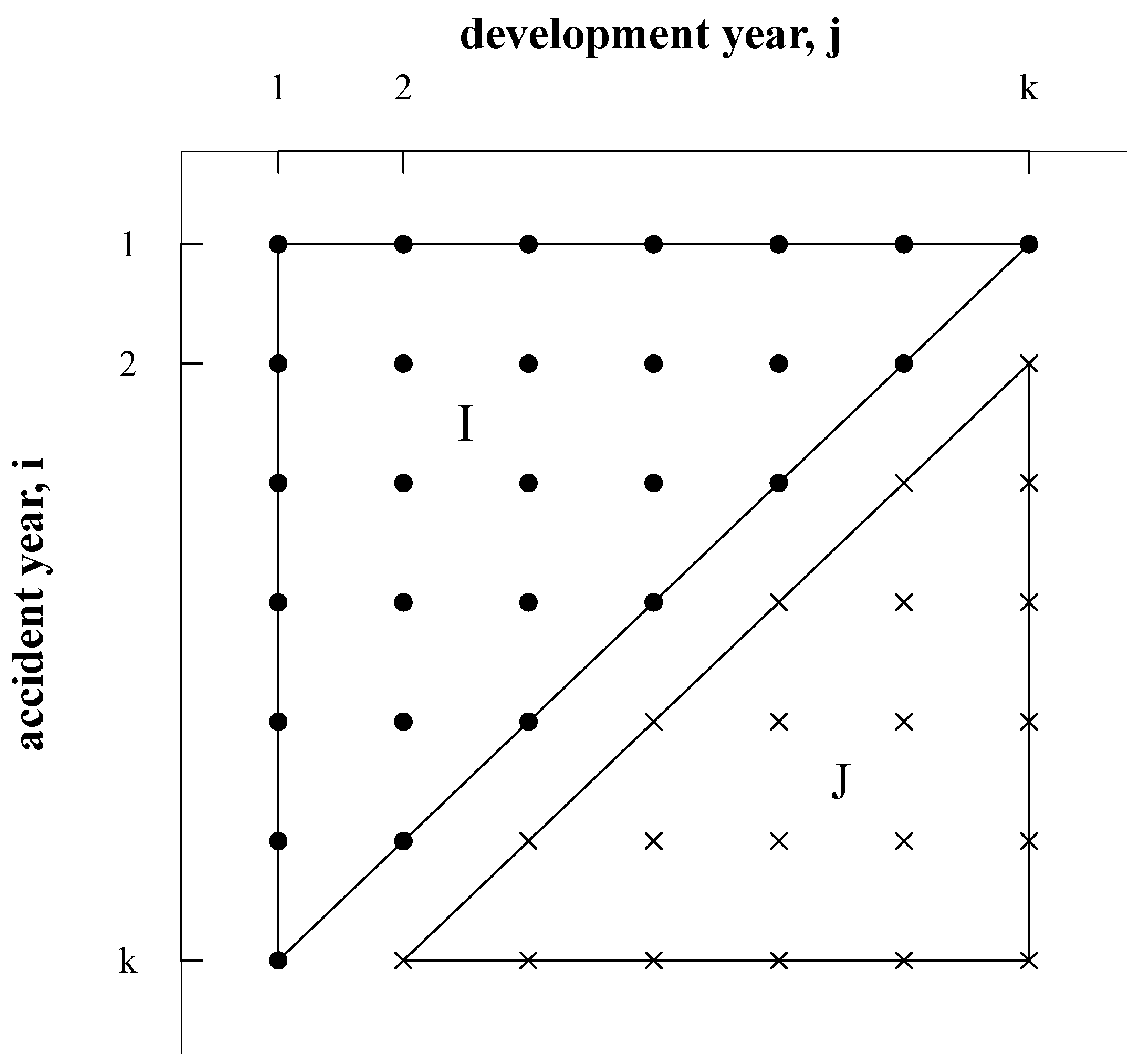
The chain ladder method is the basic actuarial tool for reserving in general insurance. This method is based on the paid run-off triangle and provides estimates for the ultimate reserve along with development factors that are used for determining cash flow. In practice, the actuary usually adjusts the ultimates using additionally available information. With the Bornhuetter et al. (1972) method the chain ladder ultimates are adjusted using prior knowledge while the adjusted cash flow is proportional to the original chain ladder cash flow. Mack (2000) gave a credibility interpretation of the Bornhuetter–Ferguson method.

The adjustment of the ultimates can be done in two ways. Either by correcting the levels of the ultimates or the relative levels of the ultimates. By this, we distinguish between the situation where the actuary has an estimate for the ultimate for a given policy year and the situation where the actuary is more comfortable with the forecast that the ultimate for a given policy year is 10% higher, say, than in the previous year. Such an estimate could, for instance, come from chain ladder analysis of incurred data. Indeed, we provide an empirical illustration where this is the case. The levels approach is most common in the literature; see for instance (Mack 2000, 2006), Taylor (2000), Verrall (2004), Wüthrich and Merz (2008) and Heberle and Thomas (2016). The relative levels approach is more recent; see (Martínez-Miranda et al. 2013, 2015).

There are potentially two concerns with the traditional Bornhuetter–Ferguson correction. It may move the reserves too much, and the cash flow distribution is not adjusted in light of the external information. Verrall (2004) addressed this in a Bayesian setup and Mack (2006) proposed an alternative approach where new weights are computed by combining actual payments and the externally estimated reserves.

Our proposal is related to that of Mack (2006), but with weights derived from a likelihood function. Adjusting relative ultimates as opposed to level ultimates is natural when working with the likelihood function in the same way as traditional chain ladder development factors are concerned with relative effects. A feature of our approach is, therefore, that external information is linked directly to the parameters of the underlying Poisson model and it is possible to express the Bornhuetter–Ferguson adjustment in terms of adjustments to the development factors. Another feature of this approach is that we can evaluate how much the adjustment moves the reserves and establish inequalities relating our approach and the traditional Bornhuetter–Ferguson adjustments.

A fundamental interpretation of the Bornhuetter–Ferguson method arises when combining chain ladder with credibility formulas. Credibility formulas have been investigated in reserving by, for instance, de Vylder (1982), Mack (2000). and more recently, Bühlmann and Moriconi (2015). We have been particularly influenced by Mack (2000), who gives a credibility formula showing that adjusting the ultimates with prior knowledge yields a partial adjustment of the reserves. He then continues to show that the iterations of the credibility formula leads to the Benktander (1976) approach. These ideas are taken a step further by Gigante et al. (2013), whereas Taylor (2000) and Wüthrich and Merz (2008) give general overviews of the Bornhuetter–Ferguson method. Our first contribution is to show that the credibility formula also applies when adjusting the relative levels of the ultimates.

It is useful to recall that the chain ladder method has the nice interpretation as maximum likelihood in a Poisson model. Kremer (1985) (see also Mack 1991) showed that the chain ladder forecasts are maximum likelihood. These forecasts are the product of observed accident year row sums and functions of the development factors; see (4). Renshaw and Verrall (1998) showed that the development factors themselves are maximum likelihood estimators in a conditional Poisson model conditioning on row sums, while Kuang et al. (2009) showed that they are also maximum likelihod in the unconditional Poisson model. The maximum likelihood result means that it is possible to compute the chain ladder estimates using generalised linear model methods. In practice the Poisson assumption is not realistic as the paid data typically have considerable over-dispersion; see for instance England and Verrall (2002). Nonetheless, the chain ladder method provides good reserve estimates that are, at least, anchored in a quasi-likelihood.

The main idea of our approach is to impose the externally estimated relative ultimates on the Poisson likelihood. Initially, it is useful to work with the standard parametrisation of the generalised linear model as opposed to the development factors. We can then formulate the relative ultimates’ constraint as a linear constraint on the parameters and derive maximum likelihood estimators. Subsequently, we translate these estimators into adjusted development factors.

The constrained maximum likelihood approach satisfies a monotonicity result. If, for instance, all the relative ultimates are increased relative to the chain ladder ultimates, then it follows that the reserves are increased. However, these new reserves increase less than the traditional Bornhuetter–Ferguson reserves that would arise by combining the adjusted relative ultimates with the chain ladder development factors.

In this paper we focus on classical mathematical statistics through the maximum likelihood method. Recent work in reserving has emerged in the literature using modern machine learning techniques. Kuo (2019) proposes deep neural networks to joint modelling paid data and total claims outstanding, claiming that no manual input is required during model updates or forecasting. Additionally, using neural networks Gabrielli and Wüthrich (2018) develop a “stochastic simulation machine” that generates individual claims histories of non-life insurance claims. Another individual claims approach but based on the classification and regression trees is suggested by De Felice and Moriconi (2019). Chukhrova and Johannssen (2017) describe a state space model for cumulative payments (that extend the chain ladder method) in combination with the Kalman filter.

The rest of the paper is organised as follows. In Section 2 we first describe the chain ladder forecasts in terms of the development factors and certain weights. Using this formulation we describe two Bornhuetter–Ferguson approaches in the literature: the interpretation offered by Mack (2000) that uses levels of ultimates, and the approach of Martínez-Miranda et al. (2013) using relative ultimates. From these two approaches the future cash flow is not influenced by the external information. We then present our proposed Bornhuetter–Ferguson reserves which are determined by a Poisson likelihood constrained by the external information. The formal derivation of our proposal is provided in Section 3 in the generalised, lineal model framework. Our proposal is derived as the solution of a constrained maximum likelihood approach, where the constraint is given by the imposed external information. Later, in Section 3.5 we show that the approach by Martínez-Miranda et al. (2013) is a mixed approach which combines unconstrained and constrained maximum likelihood estimators. Reserve forecasts and cash flow are described from our proposal, the mixed approach and the traditional chain ladder method. Only our proposed cash flow is affect by the external information, which is explicitly shown in terms of some pseudo development factors introduced in Section 3.6. In Section 4 we illustrate our proposal using a motor portfolio from a Greek insurer. These data include both paid and incurred triangles. In addition, an external estimate of the reserve is available so that this example nicely illustrates the practical issues that lead to the use of the Bornhuetter–Ferguson method. Conclusions and final remarks are provided in Section 5.

2. The Bornhuetter–Ferguson Problem

We present two standard Bornhuetter–Ferguson approaches. For now we will not formulate a statistical model, but just use the standard chain ladder formulas.

2.1. Data Structure

Consider a standard run-off triangle of paid amounts. The dimension is denoted k and we use the incremental form of the triangle. Each entry is denoted $Y_{ij}$ so that i is the accident year index and j is the development year index. The indices vary in the upper triangle with indices $1\le i,j\le k$ and $i+j-1\le k$. This is the area I in Figure 1. The objective is to forecast values of $Y_{ij}$ in the lower triangle with indices $1\le i,j\le k$ and $k+1\le i+j-1\le 2k-1$. This is the area J in Figure 1.

In the analysis we will be interested in row sums, column sums and rectangular sums

$$R_i=\sum _{j=1}^{k+1-i}{Y}_{ij},C_j=\sum _{i=1}^{k+1-j}{Y}_{ij},S_r=\sum _{\ell =1}^r\sum _{j=1}^{k-r}{Y}_{\ell j},$$

(1)

for $1\le i,j\le k$ and $1\le r\le k-1$. In practice the payments $Y_{ij}$ may be negative. This is at odds with the Poisson model interpretation of the chain ladder method which requires the payments to be non-negative. With the Poisson formulation we need the further requirement that the rectangular sums, the row sums and the column sums are positive Kuang et al. (2009) (Theorem 2); that is,

$$S_1,\dots ,S_{k-1},R_2,\dots ,R_k,C_2,\dots ,C_k>0.$$

(2)

We will assume these constraints throughout the paper, while noting that constraints in (2) may be satisfied even if some payments $Y_{ij}$ are negative.

2.2. Chain Ladder Method

The chain ladder method is computed from row sums or cumulative payments $R_i$ as in (1) and development factors

$$F_j=\frac{{\sum }_{i=1}^{k+1-j}{\sum }_{\ell =1}^j{Y}_{i\ell }}{{\sum }_{i=1}^{k+1-j}{\sum }_{\ell =1}^{j-1}{Y}_{i\ell }}\mathrm{for}j=2,\dots ,k.$$

(3)

The development factors are larger than one under the constraint (2) to $R_i,C_j,S_r$; see Theorem 2 in Kuang et al. (2009). The chain ladder forecasts of the amounts in the lower triangle are then

$${\tilde{Y}}_{ij}=R_i(F_j-1)\prod _{\ell =k+2-i}^{j-1}{F}_{\ell }.$$

(4)

From this we compute the reserve for accident year i, for $i=2,\dots ,k$, as

$$V_i=\sum _{j=k+2-i}^k{\tilde{Y}}_{ij}=R_i(F_i^{prod}-1)\mathrm{where}{F}_i^{prod}=\prod _{\ell =k+2-i}^k{F}_{\ell },$$

(5)

and the predicted ultimate payment as; see also Section 2.1.3 of England and Verrall (2002),

$$U_i=R_i+V_i=R_i{F}_i^{prod}\mathrm{for}i=2,\dots ,k.$$

(6)

If we use the convention that empty products are unity, this matches with $U_1=R_1$ and $V_1=0$, so that the in-sample prediction of the sum of the payments for accident year one equals the observation.

It will be convenient to express the above formulas in terms of certain weights. Thus, define weights, for $i=2,\dots ,k$, $j=k+2-i,\dots ,k$,

$$\begin{array}{ccc}\hfill W_{ij}& =& (F_j-1)\frac{{\prod }_{\ell =k+2-i}^{j-1}{F}_{\ell }}{F_i^{prod}}=\frac{F_j-1}{{\prod }_{\ell =j}^k{F}_{\ell }},\hfill \end{array}$$

(7)

$$\begin{array}{ccc}\hfill W_i& =& \frac{F_i^{prod}-1}{F_i^{prod}}=\sum _{j=k+2-i}^k{W}_{ij}.\hfill \end{array}$$

(8)

These are numbers between zero and unity when the development factors are larger than unity. The weights $W_i$ approach unity when the product of the development factors approaches infinity. We can then write the forecasts for each cell and each row in the lower triangle as

$${\tilde{Y}}_{ij}=U_i{W}_{ij},V_i=U_i{W}_i,i=2,\dots ,k.$$

(9)

These formulas show how the reserve $V_i$ can be found as a fraction of the predicted ultimate $U_i$, while $Y_{ij}$ indicates how the cash flow is distributed.

The chain ladder is maximum likelihood in a Poisson model that will be presented in Section 3. A feature of the likelihood function (25) is that it is symmetrical in the indices for accident year i and development year j. This observation leads to a new expression for the forecast of the reserve, which will be proved in the Appendix A. Traditionally, we forecast by computing row sums $R_i$ of the data and multiplying by the column wise forward factors $F_j$ as in (4). Alternatively, we can compute columns sums $C_j$ as in (1) and row-wise forward factors

$$G_i=\frac{{\sum }_{j=1}^{k+1-i}{\sum }_{\ell =1}^i{Y}_{\ell j}}{{\sum }_{j=1}^{k+1-i}{\sum }_{\ell =1}^{i-1}{Y}_{\ell j}}\mathrm{for}i=2,\dots ,k$$

(10)

and combine these to get the forecasts for the lower triangle, proved in the Appendix A,

$${\tilde{Y}}_{ij}=R_i(F_j-1)\prod _{\ell =k+2-i}^{j-1}{F}_{\ell }=C_j(G_i-1)\prod _{\ell =k+2-j}^{i-1}{G}_{\ell }.$$

(11)

2.3. Bornhuetter–Ferguson Using Levels of Ultimates

This section presents the Bornhuetter–Ferguson interpretation offered by Mack (2000); see also England and Verrall (2002) and Alai et al. (2009).

England and Verrall present the Bornhuetter–Ferguson idea as follows. Suppose we replace the chain ladder ultimate $U_i$ by an externally estimated reserve $U_i^{level}$ in the Formula (9). Then we get the level-based Bornhuetter–Ferguson reserve

$$V_i^{BF,level}=U_i^{level}{W}_i\mathrm{for}i=2,\dots ,k‥$$

(12)

Thus, the Bornhuetter–Ferguson reserve is the proportion $W_i$ of the externally estimated level of the ultimate. In a similar fashion the Bornhuetter–Ferguson cash flow is given by

$${\tilde{Y}}_{ij}^{BF,level}=U_i^{level}{W}_{ij}\mathrm{for}i=2,\dots ,k,j=k+2-i,\dots ,k..$$

(13)

The predicted ultimate payout turns out to be a convex combination of the chain ladder reserve $U_i$ and the externally generated number $U_i^{level}$. To see this, use the Formulas (6) and (8) to write the cumulated payments as $R_i=U_i/F_i^{prod}=U_i(1-W_i)$. It then follows that

$$U_i^{BF,level}=R_i+V_i^{BF,level}=U_i(1-W_i)+U_i^{level}{W}_i.$$

(14)

Mack (2000) refers to this a credibility formula and traces it back to Benktander (1976). He points out that it can be iterated by replacing $U_i^{level}$ by $U_i^{BF,level}$. Another consequence is the following ordering, assuming $0<W_i<1$,

$$U_i<U_i^{level}\Rightarrow U_i<U_i^{BF,level}<U_i^{level}.$$

(15)

2.4. Bornhuetter–Ferguson Using Relative Ultimates

This section presents the Bornhuetter–Ferguson approach of Martínez-Miranda et al. (2013). The idea is now to replace the relative ultimates rather than levels of ultimates. We then rewrite (9) as

$$V_i=R_1\frac{U_i}{U_1}{W}_i\mathrm{for}i=2,\dots ,k,$$

(16)

recalling that $U_1=R_1$. We now replace $U_i/U_1$ by some external measure $U_i^{rel}/U_1^{rel}$, which only provides information about the relative ultimates, such as the figure for year i being 10% higher than that for year $i-1$. This results in the relative level-based Bornhuetter–Ferguson reserve

$$V_i^{BF,rel}=R_1\frac{U_i^{rel}}{U_1^{rel}}{W}_i\mathrm{for}i=2,\dots ,k.$$

(17)

The corresponding cash flow is then

$${\tilde{Y}}_{ij}^{BF,rel}=R_1\frac{U_i^{rel}}{U_1^{rel}}{W}_{ij}\mathrm{for}i=2,\dots ,k,j=k+2-i,\dots ,k.$$

(18)

The relative Bornhuetter–Ferguson reserve also satisfies an actuarial credibility formula. To see this define $U_1=R_1$, write $R_i=R_1(R_i/U_1)$ and combine it with $R_i=U_i(1-W_i)$ as before, to get

$$U_i^{BF,rel}=R_i+V_i^{BF,rel}=R_1\left\{\frac{U_i}{U_1}(1-W_i)+\frac{U_i^{rel}}{U_1^{rel}}{W}_i\right\}.$$

(19)

Once again, we have the ordering, for $i=2,\dots k$ and assuming $0<W_i<1$,

$$\frac{U_i}{U_1}<\frac{U_i^{rel}}{U_1^{rel}}\Rightarrow U_i<U_i^{BF,rel}.$$

(20)

Martínez-Miranda et al. (2013) suggested that the relative external numbers could be computed from an incurred triangle. They extended this further to allow for reporting delays using a double chain ladder method. However, in the present paper we focus on the consequences of a Bornhuetter–Ferguson correction rather than how the external numbers are generated.

2.5. Proposed Bornhuetter–Ferguson Reserves

With the above approaches the future cash flow is determined by the chain ladder method through the weights $W_{ij}$ and not influenced by the external information. As argued by Verrall (2004) and Mack (2006) it may be desirable that the cash flow is also influenced by the external information. Our proposal allows the cash flow to be determined by a Poisson likelihood, constrained by the external information. Before we give the derivation it is useful to give a brief overview of the results.

The proposed Bornhuetter–Ferguson approach evolves around the chain ladder reserving Formula (11) involving column sums $C_j$ and row-wise forward factors $G_i$. Suppose we have externally given relative ultimates $U_i^{rel}/U_1^{rel}$ for $i=2,\dots ,k$, with the convention that $U_i^{rel}/U_1^{rel}=1$ for $i=1$. We then construct Bornhuetter–Ferguson row-wise forward factors

$${\Gamma }_i^{rel}=\frac{{\sum }_{\ell =1}^i(U_{\ell }^{rel}/U_1^{rel})}{{\sum }_{\ell =1}^{i-1}(U_{\ell }^{rel}/U_1^{rel})}\mathrm{for}i=2,\dots ,k.$$

(21)

In Section 3.3 we show that ${\Gamma }_i^{rel}$ naturally comes from a constrained likelihood. For now, the intuition is that the traditional development factors $F_j$, and $G_i$, are relative effects computed as ratios of sums over data rectangles of different sizes. This compensates for the fact that the data are only available in triangular form, so that column and row lengths are unbalanced. Once we impose the relative ultimates, which are relative row effects, then the unbalanced row lengths are essentially eliminated and we can capture relative row effects in a simpler fashion, as shown in (21).

The Bornhuetter–Ferguson forecasts of individual payments and of reserves are, then,

$${\tilde{Y}}_{ij}=C_j({\Gamma }_i^{rel}-1)\prod _{\ell =k+2-j}^{i-1}{\Gamma }_{\ell }^{rel},V_i^{rel}=\sum _{j=k+2-i}^k{\tilde{Y}}_{ij}.$$

(22)

3. Generalised Linear Model Framework

We present a Generalised Linear Model framework for Bornhuetter–Ferguson analysis. The usual chain ladder estimators are maximum likelihood in a Poisson model; see Kremer (1985). In practice, reserving data have considerable over-dispersion; see England and Verrall (2002), so that Poisson likelihood becomes a quasi likelihood. In the present paper this distinction is not so important as we will only be concerned with point forecasts. Now, if we maximise the likelihood while imposing constraints from external relative levels of ultimates, we get a closed form cash flow forecast that adapts to both data and the imposed constraints.

Next we describe the unconstrained and constrained Poisson likelihood. The first one provides the chain ladder forecasts without external information in Section 3.2, and the second one provides our proposed forecasts in Section 3.3. The approach of Martínez-Miranda et al. (2013) is shown in Section 3.5 as a mixed approach that combines constrained and unconstrained maximum likelihood estimates. Our proposed forecasts have an equivalent expression involving new column-wise development factors provided in Section 3.6. These development factors will be different for different accident years. For this reason we refer to them as pseudo development factors. This kind of formulation is also possible for the mixed approach, but with the standard chain ladder development factors, as we show in Section 3.7. A monotonicity result provided in Section 3.8 gives some insight about the effect that the imposed external information has on our proposed forecasts and those from the mixed approach.

3.1. Statistical Model

We assume that the incremental observations $Y_{ij}$ are independent Poissons with log expectation $\mathsf{E}{Y}_{ij}=exp({\mu }_{ij})$, where the predictor is given by

$${\mu }_{ij}={\alpha }_i+{\beta }_j+\delta .$$

(23)

Here ${\alpha }_i$ is the level of the accident year effect, ${\beta }_j$ is the level of the development year effect and $\delta$ is an overall level. The parametrisation presented in (23) does not identify the distribution, so we switch to the invariant parametrisation of Kuang et al. (2009); that is,

$${\mu }_{ij}={\mu }_{11}+\sum _{\ell =2}^i\Delta {\alpha }_{\ell }+\sum _{\ell =2}^j\Delta {\beta }_{\ell },$$

(24)

with the convention that empty sums are zero. Here $\Delta {\alpha }_i={\alpha }_i-{\alpha }_{i-1}$ is the relative accident year effect and $\Delta {\beta }_j={\beta }_j-{\beta }_{j-1}$ is the relative development year effect, while the overall level is determined by ${\mu }_{11}$. The Poisson log likelihood function is

$$\ell ({\mu }_{11},\Delta {\alpha }_i,\Delta {\beta }_j)=\sum _{1\le i,j,i+j-1\le k}\{{\mu }_{ij}{Y}_{ij}-exp({\mu }_{ij})-log(Y_{ij}!)\}.$$

(25)

This is a regular exponential family with canonical parameters ${\mu }_{11},\Delta {\alpha }_i,\Delta {\beta }_j$.

3.2. The Chain Ladder

The chain ladder arises by maximising the unconstrained likelihood. Theorem 3 in Kuang et al. (2009) shows that the maximum likelihood estimators are

$$\begin{array}{ccc}\hfill \Delta {\widehat{\alpha }}_i& =& \Delta log{R}_i+log{F}_{k+2-i}\mathrm{for}i=2,\dots k,\hfill \end{array}$$

(26)

$$\begin{array}{ccc}\hfill \Delta {\widehat{\beta }}_j& =& \Delta log{C}_j+log{G}_{k+2-j}\mathrm{for}j=2,\dots k,\hfill \end{array}$$

(27)

$$\begin{array}{ccc}\hfill {\widehat{\mu }}_{11}& =& log{R}_1-\sum _{j=2}^{k}log{F}_j.\hfill \end{array}$$

(28)

When inserting these estimators into Equation (23) we get estimators ${\widehat{\mu }}_{ij}$. In turn, the relative ultimates are estimated by

$$\frac{U_i}{U_1}=\frac{{\sum }_{j=1}^{k}exp({\widehat{\mu }}_{ij})}{{\sum }_{j=1}^{k}exp({\widehat{\mu }}_{1j})}=exp(\sum _{\ell =2}^i\Delta {\widehat{\alpha }}_{\ell })\mathrm{for}i=2,\dots k,$$

(29)

which are the relative ultimates entering in Equation (16). It is convenient to define $U_1=R_1$, as this says that the ultimate for first accident year equals the claims observed. With this definition, we find that $R_1=U_1$ is the maximum likelihood estimator for the expected ultimates $\mathsf{E}{R}_1$ for the first accident year. In turn, the maximum likelihood estimators for the ultimate levels satisfy

$$U_i=U_1\frac{U_i}{U_1}=U_{1}exp(\sum _{\ell =2}^i\Delta {\widehat{\alpha }}_{\ell })\mathrm{for}i=2,\dots k.$$

(30)

Now, insert the expression for $\Delta {\widehat{\alpha }}_i$ in (26) to get

$$U_i=U_1\prod _{\ell =2}^i(\frac{R_{\ell }}{R_{\ell -1}}{F}_{k+2-\ell })=U_1\frac{R_i}{R_1}\prod _{\ell =2}^i{F}_{k+2-\ell }=R_i\prod _{\ell =k+2-i}^k{F}_{\ell },$$

(31)

which are the ultimates in (6). Thus, in both cases the ultimate formulas are closely linked to the estimated relative accident year effects $\Delta {\widehat{\alpha }}_i$.

An additional result from Theorem 3 in Kuang et al. (2009) is that the forward factors $F_j$ and $G_i$ can be viewed as maximum likelihood estimators for certain combinations of the canonical parameters $\Delta {\beta }_j$ and $\Delta {\alpha }_i$, respectively. These combinations are, for $i,j=2,\dots ,k$,

$${\Phi }_j=\frac{{\sum }_{\ell =1}^{j}exp({\sum }_{h=2}^{\ell }\Delta {\beta }_h)}{{\sum }_{\ell =1}^{j-1}exp({\sum }_{h=2}^{\ell }\Delta {\beta }_h)},{\Gamma }_i=\frac{{\sum }_{\ell =1}^{i}exp({\sum }_{h=2}^{\ell }\Delta {\alpha }_h)}{{\sum }_{\ell =1}^{i-1}exp({\sum }_{h=2}^{\ell }\Delta {\alpha }_h)},$$

(32)

with the convention that empty sums are zero. The development factors are the corresponding maximum likelihood estimators; that is, $F_j={\widehat{\Phi }}_j$ and $G_i={\widehat{\Gamma }}_i$.

3.3. Imposing External Information on the Relative Ultimates

Suppose some external values are available for the relative ultimates, $U_i^{rel}/U_1^{rel}$. Equivalently, we have external values for the relative accident year effects $\Delta {\alpha }_i^{†}$; that is,

$$\Delta {\alpha }_i^{†}=log(U_i^{rel}/U_{i-1}^{rel}).$$

(33)

We could impose these as a constraint on the likelihood (25). The constraint is linear and the likelihood remains that of a regular exponential family.

The constrained maximum likelihood estimators have a simple analytical form. In line with the parameters ${\Gamma }_i$ defined in (32), define

$${\Gamma }_i^{†}=\frac{{\sum }_{\ell =1}^{i}exp({\sum }_{h=2}^{\ell }\Delta {\alpha }_h^{†})}{{\sum }_{\ell =1}^{i-1}exp({\sum }_{h=2}^{\ell }\Delta {\alpha }_h^{†})}.$$

(34)

We then have the following result, which is proven in the Appendix A.

Theorem 1.

Consider the Poisson likelihood (25) with known $\Delta {\alpha }_i=\Delta {\alpha }_i^{†}$ for $i=2,\dots ,k$ and define ${\Gamma }_i^{†}$ as (32), computed using $\Delta {\alpha }_i^{†}$. The constrained maximum likelihood estimator is unique if and only if $C_j>0$ for all $j=1,\dots k$ and given by

$$\begin{array}{ccc}\hfill \Delta {\widehat{\beta }}_j^{†}& =\Delta log{C}_j+log{\Gamma }_{k+2-j}^{†}\hfill & forj=2,\dots ,k,\hfill \end{array}$$

(35)

$$\begin{array}{cccc}\hfill {\widehat{\mu }}_{11}^{†}& =log{C}_1-log\{1+\sum _{i=2}^{k}exp(\sum _{\ell =2}^i\Delta {\alpha }_{\ell }^{†})\}\hfill & \hfill =& log{C}_1-\sum _{\ell =2}^{k}log{\Gamma }_{\ell }^{†}.\hfill \end{array}$$

(36)

As a consequence, the out-of-sample forecast from the constrained chain ladder has a simple explicit form, as shown in the following result, which is proven in the Appendix A. The result resembles the forecast in the unrestricted chain ladder computed from column sums and row-wise development factors as described in (11).

Theorem 2.

Consider the setup in Theorem 1. Point forecasts for the lower triangle are given by

$${\tilde{Y}}_{ij}^{†}=C_j({\Gamma }_i^{†}-1)\prod _{\ell =k+2-j}^{i-1}{\Gamma }_{\ell }^{†}.$$

(37)

We can now compute a Bornhuetter–Ferguson reserve based on Theorem 2. For each accident year we get

$$V_i^{†}=\sum _{j=k+2-i}^k{\tilde{Y}}_{ij}^{†}.$$

(38)

In the case where we impose external relative ultimates, the above expressions reduce to those presented previously in (22). In the above expression the notation reflects that the external information is concerned with the relative accident year parameters $\Delta {\alpha }_i^{†}$. Now, suppose the relative ultimates $U_i^{rel}/U_1^{rel}$ are taken as given. We then apply the Formula (30) to get cumulated relative accident parameters $exp({\sum }_{\ell =2}^i\Delta {\alpha }_{\ell }^{†})=U_i^{rel}/U_1^{rel}.$ Inserting this in the expression (34) for ${\Gamma }_i^{†}$ in (34) gives

$${\Gamma }_i^{†}=\frac{{\sum }_{\ell =1}^{i}exp({\sum }_{h=2}^{\ell }\Delta {\alpha }_h^{†})}{{\sum }_{\ell =1}^{i-1}exp({\sum }_{h=2}^{\ell }\Delta {\alpha }_h^{†})}=\frac{{\sum }_{\ell =1}^i{U}_{\ell }^{rel}/U_1^{rel}}{{\sum }_{\ell =1}^{i-1}{U}_{\ell }^{rel}/U_1^{rel}}={\Gamma }_i^{rel},$$

(39)

which is the expression for ${\Gamma }_i^{rel}$ in (21). Since ${\Gamma }_i^{†}={\Gamma }_i^{rel}$ we see that the point forecast ${\tilde{Y}}_{ij}^{†}$ in (37) equals the point forecast ${\tilde{Y}}_{ij}$ in (22). In turn the reserve $V_i^{†}$ in (38) equals the reserve $V_i^{rel}$ in (22).

3.4. Implementation in GLM Software

The constrained model can also be estimated using ready-made algorithms for generalised linear models. The analysis presented above shows that the constrained model is a regular exponential family so the algorithms should perform well.

For the implementation we organise the triangle Y as a vector $\mathbf{Y}$, say, of dimension $k(k+1)/2$. A design matrix $\mathbf{X}$ can be constructed from the formula (24). It has dimension $\{k(k+1)/2\}\times (2k-1)$ and the row corresponding to entry $i,j$ is given by

$$X_{ij}^{\prime }=\{1,1_{(2\le i)},\dots ,1_{(k\le i)},1_{(2\le j)},\dots ,1_{(k\le j)}\},$$

(40)

where the indicator function $1_{(m\le i)}$ takes the value unity if $m\le i$ and zero otherwise. The unrestricted model is then estimated through a generalised linear model regression of $\mathbf{Y}$ on $\mathbf{X}$ using the Poisson distribution with a log-link function.

In the constrained model the parameters ${\theta }_{known}={(\Delta {\alpha }_2^{†},\dots ,\Delta {\alpha }_k^{†})}^{\prime }$ are known. Deleting the corresponding columns from $\mathbf{X}$ gives a design matrix ${\mathbf{X}}_{reduced}$ with k columns. The deleted columns are collected as ${\mathbf{X}}_{known}$, say. The model is then estimated as a generalised linear model regression of $\mathbf{Y}$ on ${\mathbf{X}}_{reduced}$ using the Poisson distribution with a log-link function and offset given by ${\mathbf{X}}_{known}{\theta }_{known}$.

3.5. A Mixed Approach

By now we have two maximum likelihood approaches: the classical chain ladder and the restricted maximum likelihood approach derived above. These give different point forecasts for the lower triangle. A third type of point forecast arises from the Bornhuetter–Ferguson double chain ladder (BDCL) method in Martínez-Miranda et al. (2013). In the following it is shown how the three are connected.

Let us first summarise the results we obtained so far in terms of the log likelihood. In the classical chain ladder approach, we maximise the unrestricted likelihood in (25), which leads to the unrestricted estimator

$$\widehat{\xi }=\underset{\xi }{max}\ell (\xi )={({\widehat{\mu }}_{11},\Delta {\widehat{\alpha }}_i,\Delta {\widehat{\beta }}_j)}^{\prime }.$$

(41)

The restricted likelihood from Section 3.3 with restriction $\Delta {\alpha }_i=\Delta {\alpha }_i^{†}$ has a restricted likelihood maximum likelihood estimator given by

$${\widehat{\xi }}^{†}=\underset{\xi :\Delta \alpha =\Delta {\alpha }^{†}}{max}\ell (\xi )={({\widehat{\mu }}_{11}^{†},\Delta {\alpha }_i^{†},\Delta {\widehat{\beta }}_j^{†})}^{\prime }.$$

(42)

Notice, that if $\Delta {\alpha }_i^{†}=\Delta {\widehat{\alpha }}_i$, then ${\widehat{\mu }}_{11}^{†}={\widehat{\mu }}_{11}$ and $\Delta {\widehat{\beta }}_j^{†}=\Delta {\widehat{\beta }}_j$.

A third estimator is achieved by mixing the above estimators. This combines the unrestricted estimators for ${\mu }_{11}$ and ${\beta }_j$ with the given $\Delta {\alpha }_i^{†}$, such that

$${\widehat{\xi }}^{‡}={({\widehat{\mu }}_{11},\Delta {\alpha }_i^{†},\Delta {\widehat{\beta }}_j)}^{\prime }.$$

(43)

In the following, parameters resulting from this mixed approach will be marked with the index “‡,” just as parameters resulting from the constrained method will be marked with “†.” The forecast for future payments computed from ${\widehat{\xi }}^{‡}$ is

$${\tilde{Y}}_{ij}^{‡}=exp({\widehat{\mu }}_{11}+\sum _{h=2}^i\Delta {\alpha }_h^{†}+\sum _{h=2}^j\Delta {\widehat{\beta }}_h).$$

(44)

In the Appendix A we prove the identities

$${\tilde{Y}}_{ij}^{‡}={\tilde{Y}}_{ij}\frac{exp({\sum }_{h=2}^i\Delta {\alpha }_h^{†})}{exp({\sum }_{h=2}^i\Delta {\widehat{\alpha }}_h)}={\tilde{Y}}_{ij}^{†}\frac{{\sum }_{\ell =2}^{k+1-j}exp({\sum }_{h=2}^{\ell }\Delta {\alpha }_h^{†})}{{\sum }_{\ell =2}^{k+1-j}exp({\sum }_{h=2}^{\ell }\Delta {\widehat{\alpha }}_h)}.$$

(45)

In the case when the known accident parameters are derived by applying chain ladder on the incurred data, such that $\Delta {\alpha }_i^{†}=\Delta {\widehat{\alpha }}_i^{inc}$, this method gives exactly the same results as the Bornhuetter–Ferguson double chain ladder (BDCL) method in Martínez-Miranda et al. (2013).

The log likelihood function evaluated in the three points satisfies

$$\ell (\widehat{\xi })\ge \ell ({\widehat{\xi }}^{†})\ge \ell ({\widehat{\xi }}^{‡}).$$

The first inequality holds since $\widehat{\xi }$ is maximum likelihood, while ${\widehat{\xi }}^{†}$ is restricted maximum likelihood. The second inequality holds since ${\widehat{\xi }}^{‡}$ satisfies the restriction, but it is not maximum likelihood.

3.6. Pseudo Development Factors

It is common practice to think about the classical chain ladder method in terms of row sums $R_i$ and column wise development factors $F_j$ given in (1) and (3). For the restricted maximum likelihood approach there are no natural development factors in a maximum likelihood sense. Since development factors are important in daily actuarial work it is of interest to develop pseudo-development factors that keep the chain ladder pattern.

In the classical chain ladder, the forecasts for the lower triangle are computed using the Formula (11) by forwarding the row sums $R_i$ using the factors $F_j$. However, in this classical setting the predicted value for the row sum equals the row sum. In the likelihood analysis, this stems from a likelihood equation of the type $R_i=\mathsf{E}(R_i)$; see Equation (20) in Kuang et al. (2009). Thus, we can also interpret the chain ladder forecast as forwarding the predicted row sums.

Once we have imposed external information on the relative ultimates, then the forecast changes and we break the link to the original row sums and development factors. We can, however, construct pseudo forecasts of the row sums and pseudo forward factors that satisfy a relationship like (11) but with the new forecasts.

Under the constraint that $\Delta \alpha =\Delta {\alpha }^{†}$ we compute estimates ${\widehat{\mu }}_{11}^{†}$ and $\Delta {\widehat{\beta }}_j^{†}$ using (35) and (36) in Theorem 1. From these we compute pseudo forward factors from (32); that is,

$$F_j^{†}=\frac{{\sum }_{\ell =1}^{j}exp({\sum }_{h=2}^{\ell }\Delta {\widehat{\beta }}_h^{†})}{{\sum }_{\ell =1}^{j-1}exp({\sum }_{h=2}^{\ell }\Delta {\widehat{\beta }}_h^{†})},$$

(46)

and a pseudo first row sum from (28) as

$$log{R}_1^{†}={\widehat{\mu }}_{11}^{†}+\sum _{j=2}^{k}log{F}_j^{†},$$

(47)

and then the remaining pseudo row sums from (26) as

$$\Delta log{R}_i^{†}=\Delta {\alpha }_i^{†}-log{F}_{k+2-i}^{†}.$$

(48)

We show in the Appendix A that the forecast from (37) can be computed as

$${\tilde{Y}}_{ij}^{†}=R_i^{†}(F_j^{†}-1)\prod _{\ell =k+2-i}^{j-1}{F}_{\ell }^{†}.$$

(49)

The above formulas for predicted reserve and the cash flow can also be written in the credibility format we saw in (17) and (18). To see this introduce the weights

$$W_{ij}^{†}=(F_j^{†}-1)\frac{{\prod }_{\ell =k+2-i}^{j-1}{F}_{\ell }^{†}}{F_i^{prod†}},W_i^{†}=\frac{F_i^{prod†}-1}{F_i^{prod†}},$$

where, as before, $F_i^{prod†}={\prod }_{\ell =k+2-i}^k{F}_{\ell }^{†}$. Introducing the ultimates and relative ultimates

$$U_i^{†}=R_i^{†}{F}_i^{prod†},\frac{U_i^{†}}{U_{i-1}^{†}}=\frac{R_i^{†}}{R_{i-1}^{†}}{F}_{k+2-i}^{†}=exp(\Delta {\alpha }_i^{†})$$

we can then write the predicted reserve and cash flow as

$${\tilde{Y}}_{ij}^{†}=U_i^{†}{W}_{ij}^{†},V_i^{†}=U_i^{†}{W}_i^{†}.$$

3.7. Chain Ladder Forecasts with the Mixed Approach

In the mixed approach we follow a similar procedure to satisfy a relationship like (11) in order to obtain the new forecasts. The difference to the constrained method is that we can keep the forward factors from the unconstrained chain ladder model, $F_j$. However, we need to construct pseudo row sums $R_i^{‡}$ as follows.

We fix the pseudo first row sum as

$$log{R}_1^{‡}=log{R}_1,$$

(50)

and then compute the remaining pseudo row sums from (26) as

$$\Delta log{R}_i^{‡}=\Delta {\alpha }_i^{†}-log{F}_{k+2-i}.$$

(51)

We show in the Appendix A that the forecast from (44) can be computed as

$${\tilde{Y}}_{ij}^{‡}=R_i^{‡}(F_j-1)\prod _{\ell =k+2-i}^{j-1}{F}_{\ell }.$$

(52)

The forecast can be written in terms of weights, as before. Since the cash flow is derived from the chain ladder development factors, the weights are as defined in (7) and (8). In particular we have the ultimates and relative ultimates

$$U_i^{‡}=R_i^{‡}{F}_i^{prod},\frac{U_i^{‡}}{U_{i-1}^{‡}}=\frac{R_i^{‡}}{R_{i-1}^{‡}}{F}_{k+2-i}=exp(\Delta {\alpha }_i^{†}).$$

We can then write the forecast of future payments and the cash flow as

$${\tilde{Y}}_{ij}^{‡}=U_i^{‡}{W}_{ij},V_i^{‡}=U_i^{‡}{W}_i.$$

(53)

3.8. Monotonicity

The idea of the Bornhuetter–Ferguson approach is to first compute the chain ladder, and then adjust it by imposing values for the ultimates. This is a quite complicated approach and it is not immediately clear what the effect is. However, when all adjustments are in the same direction it is actually possible to show a monotonicity result for the effect of the Bornhuetter–Ferguson adjustment.

Let us consider the case when the known accident parameters, $\Delta {\alpha }_i^{†}$, are bigger than the accident parameters we obtain from the chain ladder method on paid data, $\Delta {\widehat{\alpha }}_i$. The following theorem, proved in the Appendix A, shows monotonicity results regarding the remaining parameters given in Theorem 1, and the resulting forecasts we obtain from the constrained approach in Section 3.3, ${\tilde{Y}}_{ij}^{†}$, and the mixed approach in Section 3.5, ${\tilde{Y}}_{ij}^{‡}$.

Theorem 3.

Suppose $\Delta {\alpha }_i^{†}>\Delta {\widehat{\alpha }}_i$ for all $2\le i\le k$. Then,

(a) 

${\Gamma }_i^{†}>G_i$ for all $2\le i\le k$;

(b) 

$\Delta {\widehat{\beta }}_j^{†}>\Delta {\widehat{\beta }}_j$ for all $2\le j\le k$;

(c) 

${\widehat{\mu }}_{11}^{†}<{\widehat{\mu }}_{11}$;

(d) 

${\tilde{Y}}_{ij}^{‡}>{\tilde{Y}}_{ij}^{†}>{\tilde{Y}}_{ij}$ for all $i,j$ so that $k<i+j-1<2k$;

(e) 

$F_j^{†}>F_j$ for all $2\le j\le k$;

(f) 

$R_i^{‡}>R_i^{†}$ for all $2\le i\le k$;

(g) 

$R_i^{‡}>R_i$ for all $2\le i\le k$.

To interpret this, suppose all imposed relative ultimates $U_i^{rel}/U_{i-1}^{rel}=exp(\Delta {\alpha }_i^{†})$ are larger than the chain ladder forecasts of the relative ultimates $U_i/U_{i-1}=exp(\Delta {\widehat{\alpha }}_i)$. Suppose also that the imposed relative ultimates are taken from incurred estimates as in the Bornhuetter–Ferguson double chain ladder (BDCL) method in Martínez-Miranda et al. (2013). We then get that the point forecasts for the lower triangle are ordered so that the Bornhuetter–Ferguson double chain ladder forecast ${\tilde{Y}}_{ij}^{‡}$ is larger than the Bornhuetter–Ferguson-restricted maximum likelihood forecast ${\tilde{Y}}_{ij}^{†}$, which is larger than the chain ladder forecast ${\tilde{Y}}_{ij}$. This will be the situation in the empirical illustration in Section 4.

4. Empirical Illustration

We illustrate the new methods by an example where the external knowledge comes from incurred payments. In practice, the external knowledge may also come from incurred counts, from other business lines or from other sources.

We used data from a Greek non-life insurer for motor third party liability, aggregated over bodily injury and property damage. The data are presented as cumulative run-off triangles for accident years from 2005 to 2013.

Table 1. Payments in Euros.

2005	34,492,471	47,124,007	55,244,404	59,817,460	62,550,940	66,042,036	69,311,560	70,992,659	72,265,079
2006	39,467,733	54,003,286	61,349,336	69,986,825	76,412,887	81,768,759	86,684,598	90,726,054
2007	38,928,855	57,087,550	65,905,902	77,128,507	84,158,380	92,436,441	97,838,371
2008	34,202,332	50,932,726	60,560,484	68,566,905	76,409,739	82,082,804
2009	35,657,409	52,397,264	59,849,582	66,698,806	72,724,524
2010	25,404,394	37,040,589	42,371,049	50,709,319
2011	21,268,516	31,311,410	35,973,015
2012	17,404,447	27,786,399
2013	17,676,374

shows payments, while

Table 2. Incurred amounts in Euros.

2005	54,018,141	56,699,807	60,273,204	61,112,600	63,729,660	67,142,341	69,733,859	71,980,196	72,738,376
2006	68,706,483	70,534,436	70,254,136	75,919,965	77,900,147	83,401,774	88,690,144	92,171,660
2007	64,613,205	72,600,950	76,163,387	82,388,057	87,424,383	96,246,891	102,854,340
2008	58,071,632	66,701,421	69,420,629	75,280,537	81,978,240	89,923,269
2009	60,368,719	67,868,349	72,528,239	80,726,223	85,339,588
2010	47,282,519	56,488,940	60,896,832	65,900,623
2011	49,905,225	54,801,141	60,026,903
2012	48,425,940	52,652,928
2013	47,449,977

shows incurred amounts.

Table 3. Estimates.

$\mathbf{\Delta }{\widehat{\mathit{\alpha }}}_{\mathit{i}}$	$\mathbf{\Delta }{\mathit{\alpha }}_{\mathit{i}}^{†}$	$\mathbf{\Delta }{\widehat{\mathit{\beta }}}_{\mathit{j}}$	$\mathbf{\Delta }{\widehat{\mathit{\beta }}}_{\mathit{j}}^{†}$
0.24526809	0.247261682	−0.80044252	−0.76965582
0.11149938	0.145178053	−0.68857388	−0.65777806
−0.12057425	−0.077312634	0.02370846	0.06137844
−0.04769497	0.027019249	−0.32208939	−0.29855013
−0.27637689	−0.204202408	−0.05908884	−0.03399479
−0.21412347	−0.018592530	−0.22363447	−0.20684905
−0.11353717	−0.078902778	−0.37786842	−0.36440835
−0.08135422	−0.005083078	−0.68021278	−0.67909386
${\widehat{\mu }}_{11}=17.18463300$		${\widehat{\mu }}_{11}^{†}=17.00538277$

shows parameter estimates for the paid data computed using the chain ladder and the Bornhuetter–Ferguson constrained model. For the moment we focus on the canonical parameters $\Delta {\alpha }_i$ for the relative accident year effect, $\Delta {\beta }_j$ for the relative development year effect and ${\mu }_{11}$ for the overall level. First, the chain ladder estimates are reported as $\Delta {\widehat{\alpha }}_i$, $\Delta {\widehat{\beta }}_j$ and $\Delta {\widehat{\mu }}_{11}$. Second, for the constrained model we first applied chain ladder to the incurred data. The estimates for the relative accident year effect are reported as $\Delta {\alpha }_i^{†}$. The estimates $\Delta {\widehat{\beta }}_j^{†}$ and $\Delta {\widehat{\mu }}_{11}^{†}$ were then computed from the paid data using Theorem 1. We note that the ordering $\Delta {\alpha }_i^{†}>\Delta {\widehat{\alpha }}_i$ applies for these data for all $i=2,\dots ,k=9$. Thus, the monotonicity results from Theorem 3 apply. In particular, we see that $\Delta {\widehat{\beta }}_j^{†}>\Delta {\widehat{\beta }}_j$ for all $j=2,\dots ,k=9$ and ${\widehat{\mu }}_{11}^{†}<{\widehat{\mu }}_{11}$ in Table 3.

A third approach is to use the mixed approach outlined in Section 3.5. Here we use the external estimate $\Delta {\alpha }_i^{†}$ for the relative accident year effects along with the chain ladder estimates $\Delta {\widehat{\beta }}_j$ and $\Delta {\widehat{\mu }}_{11}$. When the external estimate is based on the incurred data, as in here, this is the same as the Bornhuetter–Ferguson double chain ladder (BDCL) approach of Martínez-Miranda et al. (2013).

Table 4. Row sums and forward factors.

i,j	${\mathit{R}}_{\mathit{i}}$	${\mathit{R}}_{\mathit{i}}^{†}$	${\mathit{R}}_{\mathit{i}}^{‡}$	${\mathit{F}}_{\mathit{j}}$	${\mathit{F}}_{\mathit{j}}^{†}$
1	72,265,079	63,989,145	72,265,079
2	90,726,054	80,309,654	90,907,105	1.449130	1.463172
3	97,838,371	80,309,654	101,391,484	1.155676	1.163975
4	82,082,804	77,559,430	88,824,492	1.137937	1.149793
5	72,724,524	73,428,364	84,802,647	1.087838	1.096652
6	50,709,319	54,589,726	63,556,691	1.076112	1.085188
7	35,973,015	46,603,309	54,823,701	1.056555	1.063832
8	27,786,399	37,000,367	43,839,471	1.036684	1.041678
9	17,676,374	25,159,556	30,098,881	1.017923	1.020288

presents the estimated (pseudo) forward factors and the (pseudo) row sums. For the chain ladder, we have the observed row sums $R_i$ and the traditional forward factors $F_j$ computed by (1) and (3). For the Bornhuetter–Ferguson constrained model we have the pseudo row sums $R_i^{†}$ and the pseudo forward factors $F_j^{†}$ computed by (46)–(48). For the mixed approach we have the pseudo row sums $R_i^{‡}$ computed by (50) and (51) and the traditional forward factors $F_j$. Once again we see that the monotonicity results from Theorem 3 apply so that $R_i^{‡}>R_i^{†}$ and $F_j^{†}>F_j$.

Table 5. Reserves in million Euros.

${\sum }_{\mathit{i}=1}^{\mathit{k}}{\mathit{V}}_{\mathit{i}}$	External Valuation	${\sum }_{\mathit{i}=1}^{\mathit{k}}{\mathit{V}}_{\mathit{i}}^{†}$	${\sum }_{\mathit{i}=1}^{\mathit{k}}{\mathit{V}}_{\mathit{i}}^{‡}$
110.1	137	149.1	156.6

shows the reserves resulting from the classical chain ladder method, ${\sum }_{i=2}^k{V}_i$ from (5); the constrained approach, ${\sum }_{i=2}^k{V}_i^{†}$ from (38); and the mixed approach, ${\sum }_{i=2}^k{V}_i^{‡}$ from (53). We see that the ordering from Theorem 3 applies. For comparison we note that this portfolio was evaluated at 137 million by an external actuary, with the comment that this figure may be slightly too low. This valuation is based on the information that since 2009, the case reserves incurred were gradually increased, but the gap between incurred and paid reserves was not fully closed as of 2014. In light of this, the Bornhuetter–Ferguson constrained method appears to apply rather well in this situation.

5. Conclusions

The paper introduces a Bornhuetter–Ferguson approach that replaces the relative ultimates rather than levels of ultimates. This approach has been suggested in the Bornhuetter–Ferguson double chain ladder (BDCL) method in Martínez-Miranda et al. (2013). The traditional Bornhuetter–Ferguson method uses chain ladder weights, whereas we have estimated weights.

We made use of the fact that the chain ladder method has a nice interpretation as maximum likelihood in a Poisson model, and we formulated the relative ultimates constraint as a linear constraint on the parameters and derived maximum likelihood estimators. Furthermore, we followed this approach to reproduce the results of the BDCL method in a mixed approach, combining the constrained method with the classical chain ladder.

Monotonicity results compare the constrained method, the mixed approach and the original chain ladder results. An example illustrates the mentioned results with data from a Greek general insurer. The example shows that, when comparing all methods mentioned above, including chain ladder, the reserve given by the constrained method is in fact the closest estimate to the number given by an external expert.

Our proposal incorporates prior knowledge in a transparent way, keeping the standard principles of maximum likelihood and its well known mathematical properties. In this sense we recommend our approach over traditional Bornuetter-Ferguson adjustments as a formal statistical method for the same purpose, which keeps the simplicity and the intuition of traditional reserving. This is further shown in the convenient formulation of the forecasts in terms of the pseudo development factors provided above. Apart from this, one would also benefit from the practical advantages of using maximum likelihood that include standard inference and distribution forecasting. This cannot be done with such a level of formality in the classical approach, while for the BDCL method it has been done using intense bootstrap techniques. Another advantage of our approach is that it can, unlike the BDCL method, be applied using only one triangle, usually the payments triangle. On the other hand, this has the disadvantage of not being able to distinguish between IBNR and RBNS reserves as the BDCL method does. Another limitation of our proposal is that it cannot handle negative cells, as it is sometimes the case in the payments triangle. Further refinements are required to deal with this problem.

An outstanding problem is to provide distribution forecasts of Bornhuetter–Ferguson adjusted reserves. In practice the data will have considerable over-dispersion. By modelling that we could complement the point forecasts with distribution forecasts. Recently, Harnau and Nielsen (2018) developed an asymptotic distribution theory for the chain ladder within an over-dispersed Poisson framework. The present situation is a special case of their setup so it could potentially be extended with Bornhuetter–Ferguson adjustments. That was beyond the scope of this paper though.

Finally, because there is a full statistical model specification incorporating prior knowledge, one could implement the same type of cash-flow data validation as in Agbeko et al. (2014), based on back-testing (see also De Felice and Moriconi 2019). However, this approach has several drawbacks, more so for small datasets. Controversy also exits about which error criteria should be considered. We did not consider empirical validation in this paper and focused on theoretical statistical properties when comparing reserving methods under the generalised linear models framework. A recent discussion on empirical validation methods in reserving can be found in Matinek (2019). These can be potentially used in the context of this paper.

References

1. Agbeko, Tony, Munir Hiabu, María Dolores Martínez-Miranda, Jens P. Nielsen, and Richard J. Verrall. 2014. Validating the Double Chain Ladder Stochastic Claims Reserving Model. Variance 8: 138–60. [Google Scholar]
2. Alai, Daniel H., Michael Merz, and Mario V. Wüthrich. 2009. Mean square error of prediction in the Bornhuetter-Ferguson claims reserving method. Annals of Actuarial Science 1: 7–31. [Google Scholar] [CrossRef] [Green Version]
3. Barndorff-Nielsen, Ole. 1978. Information and Exponential Families. New York: Wiley. [Google Scholar]
4. Benktander, Gunnar. 1976. An approach to credibility in calculating IBNR for casualty excess reinsurance. Actuarial Review 3: 7–8. [Google Scholar]
5. Bornhuetter, Ronald L., and Ronald E. Ferguson. 1972. The actuary and IBNR. Casualty Actuarial Society Proceedings 59: 181–95. [Google Scholar]
6. Bühlmann, Hans, and Franco Moriconi. 2015. Credibility claims reserving with stochastic diagonal effects. ASTIN Bulletin: The Journal of the IAA 45: 309–53. [Google Scholar] [CrossRef]
7. Chukhrova, Nataliya, and Arne Johannssen. 2017. State Space Models and the Kalman-Filter in Stochastic Claims Reserving: Forecasting, Filtering and Smoothing. Risks 5: 30. [Google Scholar] [CrossRef] [Green Version]
8. De Felice, Massimo, and Franco Moriconi. 2019. Claim Watching and Individual Claims Reserving Using Classification and Regression Trees. Risks 7: 102. [Google Scholar] [CrossRef] [Green Version]
9. De Vylder, Florian E. 1982. Estimation of IBNR claims by credibility theory. Insurance: Mathematics and Economics 1: 35–40. [Google Scholar] [CrossRef]
10. England, Peter D., and Richard J. Verrall. 2002. Stochastic claims reserving in general insurance. British Actuarial Journal 8: 519–44. [Google Scholar] [CrossRef]
11. Gabrielli, Andrea, and Mario V Wüthrich. 2018. An Individual Claims History Simulation Machine. Risks 6: 29. [Google Scholar] [CrossRef] [Green Version]
12. Gigante, Patrizia, Liviana Picech, and Luciano Sigalotti. 2013. Prediction error for credible claims reserves: An h-likelihood approach. European Actuarial Journal 3: 453–70. [Google Scholar] [CrossRef]
13. Harnau, Jonas, and Bent Nielsen. 2018. Over-dispersed age-period-cohort models. Journal of the American Statistical Association 113: 1722–32. [Google Scholar] [CrossRef]
14. Heberle, Jochen, and Anne Thomas. 2016. The fuzzy Bornhuetter-Ferguson method: An approach with fuzzy numbers. Annals of Actuarial Science 10: 303–21. [Google Scholar] [CrossRef]
15. Kremer, E. 1985. Einführung in die Versicherungsmathematik. Göttingen: Vandenhoeck & Ruprecht. [Google Scholar]
16. Kuang, Di, Bent Nielsen, and Jens Perch Nielsen. 2009. Chain-Ladder as Maximum Likelihood Revisited. Annals of Actuarial Science 4: 105–21. [Google Scholar] [CrossRef] [Green Version]
17. Kuo, Kevin. 2019. DeepTriangle: A Deep Learning Approach to Loss Reserving. Risks 7: 97. [Google Scholar] [CrossRef] [Green Version]
18. Mack, Thomas. 1991. A simple parametric model for rating automobile insurance or estimating IBNR claims reserves. ASTIN Bulletin: The Journal of the IAA 21: 93–109. [Google Scholar] [CrossRef] [Green Version]
19. Mack, Thomas. 2000. Credible claims reserves: The Benktander method. ASTIN Bulletin: The Journal of the IAA 30: 333–47. [Google Scholar] [CrossRef] [Green Version]
20. Mack, Thomas. 2006. Parameter estimation for Bornhuetter/Ferguson. Casualty Actuarial Society Forum Fall: 141–57. [Google Scholar]
21. Martinek, László. 2019. Analysis of stochastic reserving models by means of naic claims data. Risks 7: 62. [Google Scholar] [CrossRef] [Green Version]
22. Martínez-Miranda, María Dolores, Jens P. Nielsen, and Richard Verrall. 2013. Double Chain Ladder and Bornhuetter-Ferguson. North American Actuarial Journal 17: 101–13. [Google Scholar] [CrossRef] [Green Version]
23. Martínez Miranda, María Dolores, Jens P. Nielsen, Richard Verrall, and Mario V. Wüthrich. 2015. Double Chain Ladder, claims development inflation and zero-claims. Scandinavian Actuarial Journal 2015: 383–405. [Google Scholar] [CrossRef] [Green Version]
24. Renshaw, Arthur E., and Richard J. Verrall. 1998. A stochastic model underlying the chain-ladder technique. British Actuarial Journal 4: 903–23. [Google Scholar] [CrossRef]
25. Taylor, Gregory. 2000. Loss Reserving: An Actuarial Perspective. Norwel: Kluwer Academic Publishers. [Google Scholar]
26. Verrall, Richard J. 2004. A Bayesian Generalized Linear Model for the Bornhuetter-Ferguson of claims reserving. North American Actuarial Journal 8: 67–89. [Google Scholar] [CrossRef]
27. Wüthrich, Mario V., and Michael Merz. 2008. Stochastic Claims Reserving Methods in Insurance. New York: Wiley. [Google Scholar]
Figure 1. Illustration of data layout.
Risks 07 00119 g001