Abstract
This paper considers the Brownian perturbed Cramér–Lundberg risk model with a dividends barrier. We study various types of Padé approximations and Laguerre expansions to compute or approximate the scale function that is necessary to optimize the dividends barrier. We experiment also with a heavy-tailed claim distribution for which we apply the so-called “shifted” Padé approximation.
1. Introduction
Let us first recall the Cramér–Lundberg risk model extended with Brownian perturbation Albrecher and Asmussen (2010); Dufresne and Gerber (1991b)
Here is the initial surplus, is the linear premium rate. The ’s, are independent identically distributed (i.i.d) random variables with distribution representing nonnegative jumps arriving after independent exponentially distributed times with mean , and denotes the associated Poisson process counting the arrivals of claims on the interval . Finally, is an independent Brownian perturbation. Ruin happens when, for the first time, a jump takes below 0.
Risk theory revolved initially around evaluating and minimizing the probability of ruin. Insurance companies are also interested in maximizing company value. This lead to the study of optimal dividend policies. As suggested by de Finetti in the 1950s de Finetti (1957)—see also Miller and Modigliani (1961)—an interesting objective is that of maximizing the expected value of the sum of discounted future dividend payments until the time of ruin.
The most important class of dividend policies is that of a constant barrier at b, which modifies the surplus only when , by a lump payment bringing the surplus to b, and then keeps it there by Skorokhod reflection until the next negative jump. In financial terms, in the absence of a Brownian component, this amounts to paying out all the income while at b. In the case of Brownian perturbation, Skorokhod reflection means keeping the process above the barrier by minimal capital injections (whenever necessary), or below a barrier, by taking out dividends (if necessary) Skorokhod (1962).
In the presence of the barrier at b, the de Finetti objective (the expected value of the sum of discounted future dividend payments until ruin) has a simple expression Avram et al. (2007) in terms of the so-called “scale function” W:
where is the time of ruin, q denotes the discount rate, the total local time at b before time t, and the law of the process reflected from above at b and absorbed at 0 and below.
The scale function Bertoin (1998); Kyprianou (2014); Landriault and Willmot (2019); Suprun (1976) is defined on the positive half-line by the Laplace transform
where the “symbol” (also-called the cumulant generating function) is defined in Equation (8) in Section 2 where we provide the necessary background information, and is the unique nonnegative root of the Cramér–Lundberg equation
The scale function is continuous and increasing on Bingham (1976), (Bertoin 1998, Thm. VII.8), (Kyprianou 2014, Thm. 8.1). It may have, however, many inflection points (such an example is depicted in Figure 1), and these play an important role in the optimization of dividends Avram et al. (2007, 2015); Schmidli (2007). For convenience, is extended to be 0 on . An important fact that will be exploited is that the Laplace transform of our function has a unique non-negative pole , see Equations (3) and (4).
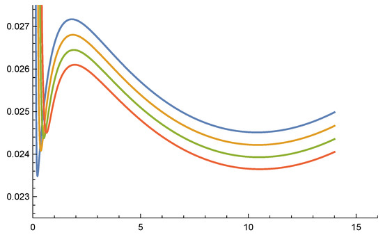
Figure 1.
Graphs of the Loeffen example for , .
This paper aims at computing/approximating the scale function , using its moments. The techniques being used are classic: Padé approximation and Laguerre expansions. The order Padé approximation of a function is a rational function in the form
for which . In the context of probability distributions, given a density function and its Laplace transform , the inverse Laplace transform of the order Padé approximant of provides a matrix exponential approximation of that matches the first moments of (including ). In Avram et al. (2011) this approach was used to approximate ruin probabilities. In this paper we develop the same approach to approximate the scale function (Section 3). An extension of the above idea is the so-called two-point Padé approximation, which allows to match not only the moments of but also the behavior of the function at 0, i.e., to match , (Section 4). For more details on this extension see Avram et al. (2018) where ruin probabilities are approximated.
Let us draw attention now to several numeric challenges which were absent in the ruin probability problem.
- Optimizing dividends starts by optimizing the so-called “barrier function”and the optimal dividend policy is often simply a barrier strategy at its maximum. This is the case in particular when the barrier function is differentiable withand has a unique local maximum ; then this yields the optimal dividend policy, and the optimal barrier function,turns out to be the largest concave minorant of .1
- The challenge of multiple inflection points. In the presence of several inflection points, however, the optimal policy is multiband Azcue and Muler (2005); Schmidli (2007); Avram et al. (2015); Loeffen (2008). The first numerical examples of multiband policies were produced in Azcue and Muler (2005); Loeffen (2008), with Erlang claims . However, it was shown in Loeffen (2008) that multibands cannot occur when is increasing after its last global minimum (i.e., when no local minima are allowed after the global minimum).Loeffen (2008) further made the interesting observation that for Erlang claims (which are non-monotone), multiband policies may occur for volatility parameters smaller than a threshold value, but barrier policies (with a non-concave value function) will occur when is large enough.Figure 1 displays the first derivative for . The last two values yield barrier policies with a non-concave value function, due to the presence of an inflection point in the interior of the interval .
Below we will investigate whether our approximations are precise enough to yield reasonable approximations for and the root(s) of .
Special features. While our methods consist essentially of Padé approximation and Laguerre–Tricomi–Weeks Laplace transform inversion, we found that exploiting the special features of our problem is useful. These are:
- including known values of (using thus two-point Padé approximations).
- shifting the approximations around specified in Equation (4), which transforms into a survival probability. As a consequence, we end up using a certain judicious choice of the Laguerre exponential decay parameter of Equation (40), which is usually left to be tuned by the user in the Laguerre–Tricomi–Weeks method Weideman (1999).
Contents. We briefly review classical ruin theory in Section 2. Padé approximations are provided in Section 3, where we also spell out the simplest algorithm for the computation of the scale function. In Section 4, we derive low-order Padé and two-point Padé approximations of , reminiscent of the de Vylder approximation of the ruin probability. Some of these approximations appeared already in Gerber et al. (2008), where however the Padé method and the fact that they can be easily extended to higher orders is not mentioned. Section 5 offers our personal strategy for inverting Laplace transforms of interest in probability, in the presence of uncertainty. Section 5.1 implements the Laguerre–Tricomi–Weeks Laplace transform inversion with a certain judicious choice of the exponential decay parameter (40), which is believed to be new. Section 6 presents numeric experiments with mixed exponential claims. Section 7 presents experiments with Pareto claims; since these have a heavy tail and, consequently, finitely many moments, we apply a “shifted” Padé approximation of the claim distribution. Section 8 includes a computer program required to obtain test cases with exact rational answers, using the Wiener–Hopf factorization; of course, this is quite convenient for the initial testing of the precision of our algorithms. Finally, Section 9 reviews a more general version of the Laguerre–Tricomi–Weeks Laplace inversion method, which may be of interest for further experiments.
2. A Short Review of Classical Ruin Theory
The process defined in Equation (1) is a particular example of spectrally negative Lévy processes, with finite mean, which are defined by assuming instead of Equation (1) that is a subordinator with -finite Lévy measure that integrates x, but having possibly infinite activity near the origin Bertoin (1998) (for Equation (1), the Lévy measure is given by ). A spectrally negative Lévy process is characterized by its Lévy–Khintchine/Laplace exponent/cumulant generating function/symbol defined by , with of the particular form
Some concepts of interest in classical risk theory are:
- First passage times below and above a level a
- The first first passage quantity to be studied historically was the eventual ruin probability:In order that the eventual ruin probability not be identically 1, the parameterwhich is called drift or profit rate, must be assumed positive.The Laplace transform of the ruin probability is explicit, given by the so-called Pollaczek–Khinchine formula, which states that the Laplace transform of is:
The roots with negative real part of the Cramér–Lundberg equation
are important, when such roots exist. They will be denoted by , and ordered by their absolute values . is called the adjustment coefficient, and furnishes the Cramér–Lundberg asymptotic approximation
Laplace transform inversion. As explained here, the first passage theory for Lévy processes with one-sided jumps reduces essentially to inverting the Laplace transform Equation (3). This applies not only to the well-known ruin probabilities, but also to intricate optimization problems involving dividends, capital gains, liquidation of subsidiary companies, etc.
Remark 1.
If the claims have a phase-type or matrix exponential distribution, then the Cramér–Lundberg equation has a finite number of roots, and Laplace transform inversion reduces to finding roots of denominators and to partial fractions, operations which are essentially exact with the current computing resources. For example, the ruin probability is provided by an exact formula (which extends the Cramér–Lundberg asymptotic approximation). With distinct roots, this is
Similar formulas hold for the scale function and related quantities (derivatives and integrals of the scale function, etc).
This refocuses the question of ruin probabilities and similar quantities to the harder cases of
- 1.
- non-matrix exponential claims,
- 2.
- when does not exist (the non-Cramér case), and
- 3.
- when not all moments exist, which we will call “heavy tails”.
For non-matrix exponential jumps, one can start by a Padé approximation of the Laplace transform, which is perhaps the oldest method of Laplace transform inversion. For heavy-tailed claims, whose moment generating function is not analytic at the origin, one may apply, as it will be shown in Section 7, a “shifted” Padé approximation before Laplace transform inversion—see, for example, Avram et al. (2018). In this paper, we also compare the precision of the classic Padé and two-point Padé Laplace transform inversion methods with the Laguerre–Tricomi–Weeks inversion, as applied to the optimal dividends barrier problem. As test cases, we consider mixed exponentials, for which exact answers are available for the case of rational Wiener–Hopf factorization roots described in Section 8.
3. Padé/matrix exponential Approximations of the Scale Function
The essence of classic ruin theory is the availability of explicit “output Laplace transforms” expressed in terms of “input Laplace transforms”, Equations see (3), (10) and (16). Equivalently, “output moments” (i.e., Taylor coefficients of functions of interest) are expressed in terms of “input data moments”. In the case of insufficient data, Padé approximations of the output function seem to deserve special attention, because they involve only a few input moments, and seem to extract at low orders the essence of the data. Note, as pointed out in Avram et al. (2011, 2018); Avram and Pistorius (2014), that the classical ruin theory approximations of Cramér–Lundberg, De Vylder and Renyi are all first order Padé approximations. Slightly increasing the order yields more sophisticated moments based approximations Avram et al. (2018); Avram and Pistorius (2014); Ramsay (1992). Similar approximations, which could be useful in dividends optimization, are presented in Section 4—see also Hu et al. (2017) for a related application to reinsurance.
With more reliable data, higher order Padé approximations are just as easy to obtain, using computer systems such as Maple, Mathematica, Sage, Matlab, etc. Let denote the moments of the Lévy measure2, and let
The simplest Padé approximation of the scale function and optimal dividend barrier requires implementing the following algorithm, which is valid for claim distributions having moments.
- Obtain the power series expansion of the Laplace exponent in terms of the moments of the Lévy measure
- Construct a Padé approximationi.e., find , by solving the linear system . As emphasized in Figure 2, the series expansion of is a good approximation only for small s; since the most important part of the approximation is the root in Equation (25), simple Padé approximation will only work for small q.
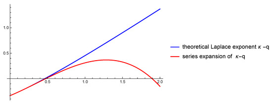 Figure 2. The series expansion of has multiple contact with at , but increases asymptotically at a smaller rate. Despite that, it yields quite reasonable approximations of , for q small enough.
 - Factor the denominator asThis operation is the essential numerical difficulty, but may be achieved nowadays with arbitrarily high precision.
- Then, partial fractions plus inversion quickly yield an approximate Laplace transform inverse
- The dividend barrier is obtained by finding the largest nonnegative root of .
Remark 2.
Remark 3.
Note that, as already mentioned in Remark 1, Padé inversion cannot be improved upon when the density of the claims is matrix exponential of some order n, (or, equivalently, when its Laplace transform is rational), since it results into the exact decomposition of the scale function into exponentials
where the are partial fraction decomposition coefficients (and where the first coefficient follows from the normalization constant chosen in Equation (3)).
The coefficients are less important than the roots, and in fact one may easily improve on Padé, for example, by recomputing them so that the approximation is optimal in sense. Positivity of the ’s, or, better, of their “Coxian linear combinations” can be further ensured by linear programming, if desired.
The preceding observations make Laplace inversion by rational approximation of the Laplace transform a quite attractive tool in ruin theory and related fields, from both a pedagogical and numerical point of view Avram et al. (2011, 2018); Avram and Pistorius (2014). One drawback is the appearance of non-admissible roots (for example, with ), which will imply non-admissible ruin probabilities for very large initial reserves x. It may be argued, however, that if the admissibility range is large enough, in practice this may not cause problems. Moreover, this problem may be fixed by convenient mathematical tools, implemented in packages such as BUTools and SOPE Bobbio et al. (2005); Dumitrescu et al. (2016); Horváth and Telek (2016).
For the sake of simplicity, we will mostly take from now on. In this case, the Pollaczek–Khinchine formula, Equation (10), may be simply expressed in terms of the so-called “excess distribution ” of the jumps, and of the “intensity” :
where The last formula is especially convenient for cases where the excess distribution is simply related to the original one, as in the case of the Pareto distribution.
We would like to note however that the Padé approach works with no problems in the presence of Brownian motion, the only modifications being the form of and the second moment of the associated Lévy measure—see Equation (13).
4. Two-Point Padé Approximations, with Low Order Examples
One may obtain better results by incorporating into the Padé approximation the following initial values, which can be derived easily from the Laplace transform:
Further derivatives at 0 could be computed, but we stop at order 2, since already requires estimating , which is a rather delicate task starting from real data.
We will provide in Proposition 1 below a couple of two-point Padé approximations, when . Before that, it is worth recalling the case of exponential claims.
Example 1.
The Cramér–Lundberg model with exponential jumps. Consider the Cramér–Lundberg model with exponential jump sizes with mean , jump rate λ, premium rate , and Laplace exponent , assuming . Let denote the adjustment coefficient, and let . Solving for s yields two distinct solutions given by
The W scale function is:
where .
Furthermore, it is well-known and easy to check that the function is in this case unimodal with global minimum at
since and that the optimal strategy for the de Finetti problem is the barrier strategy at level Avram et al. (2007).
Proposition 1.
- 1.
- To secure both the values of and , take into account Equations (17) and (18), i.e., use the Padé approximationThis yieldsIn view of Equation (20), this yields the same result as approximating the claims by exponential claims, with .
- 2.
- To ensure , we must only impose the behavior specified in Equation (17), i.e., use the Padé approximationFor , this yieldswhere we denoted by the first moment of the excess density . For exponential claims this coincides with Equation (22) (since ). This is the De Vylder B) method (Gerber et al. 2008, (5.6–5.7)), derived therein by assuming exponential claims, with , and simultaneously modifying λ to fit the first two moments of the risk process.
- 3.
- When the pure Padé approximation is applied, the first step yieldswhere is a so-called “normalized moment” Bobbio et al. (2005).This is the De Vylder A) method (Gerber et al. 2008, (5.2–5.4)), derived therein by assuming exponential claims, with , and simultaneously modifying both λ and c to fit the first three moments of the risk process.
Lemma 1.
In the case of exponential claims, the three approximations given above are exact.
Proof.
It suffices to check that for exponential claims all the normalized moments are equal to . □
In particular, the optimal barrier for exponential claims obtained by the explicit Equation (21) is the same. For example, yields
and .
5. Two Numerical Methods for Computing : The Tijms–Padé and Laguerre–Tricomi–Weeks Approximations
Computing reduces in principle to the case , if may be accurately computed, via the well-known relation
where denotes the 0-scale function with respect to the “Esscher transformed” measure (in general, the transform of the measure P of a Lévy process with Laplace exponent is the measure of the Lévy process with Laplace exponent , with r in the domain of (Albrecher and Asmussen 2010, Proposition 4.2), (Kyprianou 2014, 3.3 pg.83)).4
The Esscher transform removes the exponential growth, or, equivalently, the unique positive pole of . When working with the Esscher transform, let
denote the function after the behavior at and ∞ has been exploited5 We construct then a mixed exponential/rational approximation
For general rational approximations, we will use the name of “Esscher–Tijms type algorithms”, and for the Padé case we will use the name of “Esscher–Tijms–Padé approximation ”, in reference to the fact that the special positive pole, supposed to be known somehow exactly, has been removed.
Remark 4.
Clearly, a very precise approximation of the unique positive pole and the “moments” are an essential for determining , which was missing in the ruin probability problem. is quite easy to compute under parametric models where the Laplace transform of the jumps is explicit, as the unique positive root of a convex function. It may also be estimated empirically by the plug-in method, but this seems not yet studied in this context. We took therefore the shortcut of assuming that is available with infinite precision. Conceptually, this amount to studying the Esscher transform.
The Padé approximation of the Esscher transform is the first method we have investigated. An interesting alternative to the Esscher transform is to consider the simplified Laplace transform:
whose positive pole has been removed and thus coincides with the negative Wiener–Hopf factor (see Section 8, (44)), up to the constant .
Subsequently, we may apply a Padé (or more sophisticated rational approximation Nakatsukasa et al. (2018)), with the goal of approximating the dominant poles of the presumably imprecisely known transform.
Note that a Padé of will then yield immediately a rational approximation of and a mixed exponential approximation of . The Padé approximation requires solving
For the Cramér–Lundberg case, also fixing
leads to the linear system
Remark 5.
The “Tijms-two-point Padé approximation ” with and satisfied by Equation (28) is obtained by solving:
This is exact for the Cramér–Lundberg process with exponential jumps of rate μ, since then and reduces to the second root of the Cramér–Lundberg equation.
Starting with order two, we may also satisfy . We must now solve
Tedious computations or the help of Mathematica reveal that this is exact for the Cramér–Lundberg process with mixed exponential jumps of order 2.
In the next subsection we propose a method similar in spirit to the above: Obtaining first the simplest exponential approximation, and refining this subsequently (analogously to Step 3) above by means of applying the Laguerre–Tricomi–Weeks expansion.
5.1. Laguerre–Tricomi–Weeks Laplace Transform Inversion with Prescribed Exponent
In this section we obtain first an exponential approximation of the transformed scale function of the form , by a first order Padé approximation6 of its Laplace transform
The exponent thus obtained is the “second step output” form the previous section.
Next, apply the Tricomi–Weeks method for Laplace transform inversion (see, for example, Abate et al. (1998)), i.e., search for a Laguerre series expansion
where, following tradition, C normalizes the sum following it to be a pdf7, and where
denote the Laguerre polynomials, which are orthogonal with respect to the weight . The Laplace transform of the Laguerre polynomial is
The Laguerre–Tricomi–Weeks method is based on the fact that Equation (31) is equivalent to
Now the last RHS may be obtained using the “collocation transformation” and a power series expansion of the LHS, yielding
In conclusion, extracting the Taylor coefficients of yields approximations to by substituting it into Equation (31). After multiplication by we obtain approximations of .
Determining . Previous work on choosing involved the radius of convergence of a Laguerre–Tricomi–Weeks expansion which is slightly more general than Equation (35) Weideman (1999)—see also Section 9. We now introduce a different method.
Recall that our Laplace transform has been shifted by , so that 0 is the largest pole, and that the growth at ∞ has been removed by subtracting
Now, let
denote the mass of our measure.
A reasonable may be obtained by approximating via a first order exponential approximation of C
(or, equivalently, by fitting the first two moments of ), so that the Laguerre exponent in Equation (31) is fitted at order .
Fitting moments may be achieved by Padé’s method. At order 1, this yields
Finally, a bit of algebra yields
Remark 6.
It may also be checked that
and
This will be useful for developing higher order two-point Padé approximations of .
Remark 7.
It is possible that the choice in Equation (40) for the Laguerre–Tricomi–Weeks exponential parameter (often left to the user) has previously been proposed, but we have been unable to find this result in the literature. Note the natural generalization to the case of Laplace transforms with a finite number of positive poles (instead of a single one, as in our case).
We show in the next sections that the approximations obtained by the Tijms–Padé and Laguerre–Tricomi–Weeks methods are accurate enough so that the resulting inverse retain the features of the intricate Azcue and Loeffen examples Azcue and Muler (2005); Loeffen (2008).
5.2. Combining the Tijms–Padé and Laguerre–Tricomi–Weeks Approximations
We end this section by proposing a more general strategy for inverting and other Laplace transforms of interest in probability, given the uncertainty inherent in real world data. This consists in refining the rational approximation of Equation (26) by constructing the quotient of the original Laplace transform and its approximation
and by applying to it an inversion method with good convergence properties like Laguerre–Tricomi–Weeks. The final approximation of will be then a convolution of the inverse Laplace transforms and . This may be viewed as a to a two stage filter, aimed at removing uncertainties of different orders of magnitude.
6. Mixed Exponential Claims
We will now consider examples with rational roots. The idea for obtaining “rational first passage probabilities”, which appeared essentially in Dufresne and Gerber (1991a), is to replace the additive parametrization of Equation (8) with that provided by the so-called Wiener–Hopf factorization of Equation (44). For Cramér–Lundberg processes, it is enough to specify the negative roots and poles (for example, by specifying the Wiener–Hopf factor, Equation (44), and also the positive root of the symbol. The additive decomposition of the model’s symbol, Equation (8), may be recovered using its behavior when , and partial fractions. This is automatized in the Mathematica program RatC which is available upon request from the authors.
This package is useful for providing testing cases for our approximations, since in such examples the case of mixed exponential claims is reduced to exact rational root-solving and partial fractions (included automatically in Mathematica’s command InverseLaplaceTransform).
Example 2.
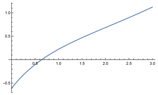
A Cramér–Lundberg model with exponential mixture jumps of order two. This example illustrates the computational steps of the previous section, and the fact that the second order Tijms approximation for mixed exponential claims of order 2 is exact (and so is in particular the optimal barrier).
We chose and a negative Wiener–Hopf factor
which is input into our Rat program—see Section 8—by specifying the interspersed roots and poles exr = (1/2, 3/2); exc = (1, 2).
This corresponds—see Section 8—to a Cramér–Lundberg process with cumulant generating function
where we used , and claim density
with mean and . The resulting scale function with is
see Figure 3, and the optimal barrier is . Recall from Remark 5 that the Tijms–Padé approximation is exact at order 2.

Figure 3.
.
After an Esscher shift of , the scale function transform becomes
with dominant non-zero pole After the removal of the pole 0, this becomes
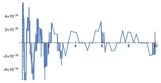
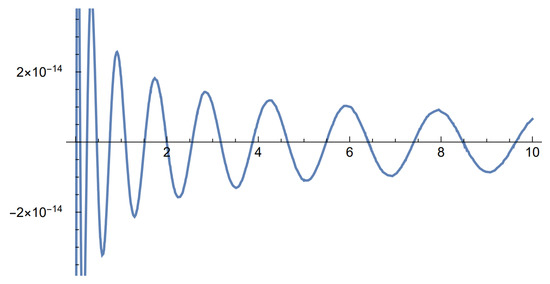
The Padé approximation of order is , the Laguerre exponent is , and the largest error with is —see Figure 4.

Figure 4.
Relative errors of the Laguerre–Tricomi–Weeks inversion with mixed exponential claims of order 2.
Example 3.
A perturbed Cramér–Lundberg model with exponential mixtures jumps of order three. Our next example is produced by taking and a negative Wiener–Hopf factor
which corresponds to the cumulant generating function:
Note that the only impact of the presence of Brownian motion with is that the degree of the numerator in Equation (42) equals the degree of the denominator .
The resulting scale function with is
The input to the Laguerre–Tricomi–Weeks inversion is
its Padé approximation of order is , the Laguerre exponent is , and the largest error with is .8 Other exponents do better however. For example, the larger exponent , where we have erased the 2 in the denominator, has a smaller larger error when of .
Example 4.
A Cramér–Lundberg model with exponential mixtures jumps of order three. Our next example is produced by taking and a negative Wiener–Hopf factor
with poles . This corresponds to a Cramér–Lundberg process with cumulant generating function:
The scale function with is
and the optimal barrier is . The Padé Tijms approximation is . The input to the Laguerre–Tricomi–Weeks inversion is
the Padé approximation of order is , the Laguerre exponent is , and the largest error with is —see Figure 5.

Figure 5.
Relative errors of the Laguerre–Tricomi–Weeks inversion with mixed exponential claims of order 3.
Again, the exponent does better, with the largest error with of . This suggests the importance of optimizing α, which is a difficult problem Giunta et al. (1989); Weideman (1999). Recall however our proposal to circumvent it by starting with a higher order Padé approximation of —see (41).
7. Padé Approximation of Heavy-Tailed Claims
In this section we experiment with heavy-tailed claims in the context of dividends barrier. To this end we consider hereby the risk process with Pareto II/Lomax claim size distribution (also known as American Pareto) with survival function given by mean and . The Laplace transform of the density is Nadarajah and Kotz (2006)
where is the incomplete gamma function and
is Tricomi’s Hypergeometric U function (Abramowitz and Stegun 1965, 13.2.5), where we used (see, (Abramowitz and Stegun 1965, 6.5.22)). It follows that the Laplace transform of the survival function is
As discussed in Albrecher et al. (2010), the model is suitable for obtaining precise quantities by numerical inverse Laplace transform using the fixed Talbot (FT) algorithm with parameter . We will refer to results obtained by the FT algorithm as “exact”.
We apply with which the distribution is of infinite variance. One can still obtain moment based Padé approximations by “shifting” the claim distribution as described in Avram et al. (2018). The resulting approximate claim density function approximations of order and 8 are the following (the shift factor we applied is 1.6):
which match moments (including ) of the shifted density.
Based on the Laplace transform of the above approximations it is straightforward to obtain the Laplace transform of and then by symbolic inverse Laplace transform itself. We studied the model with . We considered both the perturbed model with and the non-perturbed one. In the following we present figures where dots represent values obtained by numerical Laplace inversion while solid lines are given by the order 4 approximation. Figure 6 and Figure 7 gives the result for the perturbed case and Figure 8 and Figure 9 for the non-perturbed model. Numerical inverse Laplace transform requires about 60 seconds on a modern laptop to obtain a single point of while the Padé approximation is immediate. Order 4 Padé approximation provides results that are not distinguishable from the exact values. The right panels of Figure 7 and Figure 9 show that increasing the order of the approximation improves accuracy.

Figure 6.
The scale function (on the left) and its derivative (on the right) in the case of the perturbed model.

Figure 7.
On the left the expected value of total discounted dividends, , as function of b with in the case of the perturbed model. On the right the absolute error of approximations of of order 4 (blue), 6 (orange) and 8 (green).

Figure 8.
The scale function (on the left) and its derivative (on the right) in the case of the unperturbed model.

Figure 9.
On the left the expected value of total discounted dividends, , as function of b with in the case of the unperturbed model. On the right the absolute error of approximations of of order 4 (blue), 6 (orange) and 8 (green).
8. The Wiener–Hopf Factorization and Risk Theory with Rational Roots
Lévy processes are naturally parameterized via the additive decomposition of the symbol Equation (14). The roots and poles of the symbol play an important role and this has lead eventually to the discovery of the well-known Wiener–Hopf factorization Kyprianou (2014)
With mixed exponential claims of rates for example, this holds with and
where and are, respectively, the nonnegative and negative roots of the Cramér–Lundberg equation.
One may bypass the numerical difficulties of finding roots by parameterizing a risk process by the poles and roots of its Wiener–Hopf factor . To further simplify matters, one may choose them as integers; then, the parameters of the process will be rational.
The simplest illustration is provided in the tables of (Dufresne and Gerber 1991a, p. 24): The input parameters therein are the interspersed non-zero integer roots (denoted there by ) and the poles of the symbol ; essentially, this is equivalent to specifying Equation (45). The output parameter is the limit of Equation (45) when , yielding
where (Dufresne and Gerber (1991a) gives instead the safety load ). The other output parameters are partial fraction decomposition coefficients, given by the well-known partial fractions decomposition formulas, see Equation (12) for an example.9 Once these coefficients are known, it is easy to show that
Note that the Levy model of Equation (1) is overdetermined, since by scaling the time, the symbol will be multiplied by an arbitrary factor; thus, one of the parameters, for example, c, may be specified at will.
A Computer Program “Rat” That Outputs a Spectrally Negative Lévy Process with Given Roots and Poles of Its Symbol
The first program inputs consists of
- a vector of length N containing the negatives of the Cramér–Lundberg roots with negative real part, and
- a vector of length , containing the diagonal of the triangular matrix B representing the Coxian distribution (the rest of the parameters of this law are only provided indirectly, via the Cramér–Lundberg roots).
The algorithm must distinguish between four cases, depending on whether or not and , and this is achieved by different inputs. The case is specified via the presence of a third input parameter (which is 0 if ), and the cases are distinguished by having and respectively.
We will now introduce an artificial normalization constant , defined by
(the factor being incorporated just for convenience, see Equation (48)). Note that this definition allows one to deal with the case as a limiting case of . may be thought of at first as the leading coefficient of (which is c when and when ); for a more precise statement, see Equation (48).
When , we will write the symbol as
where .
With this parameterization, results when will have a limit, provided that is kept constant. If we assume (w.l.o.g.) that the polynomial part inside the parentheses in Equation (47) is monic (i.e., if and else), then the parameter equals either the original parameter c or .
Remark 8.
In terms of , we may rewrite the Wiener–Hopf factorization as
where the last factor in Equation (48) may be represented as a quotient of monic polynomials. This equation motivated the introduction of .
Remark 9.
The various components of the cumulant generating function are readily obtained: and q by extracting the polynomial part; the remaining jump part then yields .
Remark 10.
Note that if the condition
is satisfied, then the nonnegativity of the density of the jumps is ensured—see, for example, Kuznetsov et al. (2012) (this condition is also necessary with hyperexponential jumps).
If this condition is not satisfied, then the user must deal somehow with the nonnegativity by restricting the position of the Cramér–Lundberg roots (not an easy task).
The output of our program consists of several first passage characteristics:
- Eventual ruin probabilities
- Cumulants generating function (Laplace exponent) of the Levy process
- Homogeneous scale function , for one fixed q
They are most easily described as combinations of exponentials.
9. Further Background on the Laguerre–Tricomi–Weeks Method
We now proceed to review an extension of the Laguerre expansion, the “Laguerre–Tricomi–Weeks” method of inverting the Laplace transform, initially proposed by Tricomi in 1935 and McCully (see McCully (1960)), which is considered as one of the most efficient methods of inverting the Laplace transform Weideman (1999). We mention also that an exact explicit closed-form Laguerre series expansion formula was proposed recently in Zhang and Cui (2019).
Consider a given function
(note that the transformation Equation (50) corresponds to a linear transformation for the Laplace transform and its singularities). First, one attempts to construct a Laguerre expansion
with two judiciously chosen parameters and , where is the maximum real part of the singular points of .
After the change of variables , the coefficients may be found from the Taylor expansion
where is the radius of convergence of , or, equivalently,
Judicious choices of (related to maximizing ) and (related to finding a minimal circle including the singular points of ) may turn this into one of the most effective inversion methods Weideman (1999), Abate et al. (1998).
Some particular choices are , and , in which case the Taylor expansion for the coefficients becomes, respectively,
As noted by Keilson and Nunn Keilson and Nunn (1979) (see also Keilson et al. (1980, 1981)), and Abate et al. (1998), respectively, in the second and third cases, the expansion in the of powers Equation (32) implies simple relations between the Laguerre transform and another interesting technique, the Erlang transform, which is a useful tool for the solving integral equations of the convolution type. We refer to these papers for a further discussion of the relative advantages of the Erlang and Laguerre transforms, and the spaces of the functions within which they converge.
Author Contributions
F.A., A.H. and S.P. contributed equally to Conceptualization, Methodology, Formal Analysis, Investigation, Writing-Original Draft Preparation, Writing-Review, Project Administration, Supervision and Editing, and U.S. contributed to Software, Validation and Data Curation.
Funding
This research received no external funding.
Conflicts of Interest
The authors declare no conflict of interest.
References
- Abate, Joseph, Gagan L. Choudhury, and Ward Whitt. 1998. Numerical inversion of multidimensional laplace transforms by the Laguerre method. Performance Evaluation 31: 229–43. [Google Scholar] [CrossRef]
- Abramowitz, Milton, and Irene A. Stegun. 1965. Handbook of Mathematical Functions: With Formulas, Graphs, and Mathematical Tables. Mineola: Dover Publications, vol. 55. [Google Scholar]
- Albrecher, Hansjörg, and Sören Asmussen. 2010. Ruin Probabilities. Singapore: World Scientific, vol. 14. [Google Scholar]
- Albrecher, Hansjörg, Florin Avram, and Dominik Kortschak. 2010. On the efficient evaluation of ruin probabilities for completely monotone claim distributions. Journal of Computational and Applied Mathematics 233: 2724–36. [Google Scholar] [CrossRef][Green Version]
- Avram, Florin, Abhijit Datta Banik, and Andras Horváth. 2018. Ruin probabilities by padé’s method: Simple moments based mixed exponential approximations (Renyi, De Vylder, Cramér–Lundberg), and high precision approximations with both light and heavy tails. European Actuarial Journal 9: 273–99. [Google Scholar] [CrossRef]
- Avram, Florin, D. Fotso Chedom, and Andras Horváth. 2011. On moments based Padé approximations of ruin probabilities. Journal of Computational and Applied Mathematics 235: 3215–28. [Google Scholar] [CrossRef]
- Avram, Florin, Zbigniew Palmowski, and Martijn R. Pistorius. 2007. On the optimal dividend problem for a spectrally negative Lévy process. The Annals of Applied Probability 17: 156–80. [Google Scholar] [CrossRef]
- Avram, Florin, Zbigniew Palmowski, and Martijn R. Pistorius. 2015. On Gerber–Shiu functions and optimal dividend distribution for a Lévy risk process in the presence of a penalty function. The Annals of Applied Probability 25: 1868–1935. [Google Scholar] [CrossRef]
- Avram, Florin, and Martijn R. Pistorius. 2014. On matrix exponential approximations of ruin probabilities for the classic and Brownian perturbed Cramér-Lundberg processes. Insurance: Mathematics and Economics 59: 57–64. [Google Scholar] [CrossRef]
- Azcue, Pablo, and Nora Muler. 2005. Optimal reinsurance and dividend distribution policies in the Cramér-Lundberg model. Mathematical Finance 15: 261–308. [Google Scholar] [CrossRef]
- Bertoin, Jean. 1998. Lévy Processes. Cambridge: Cambridge University Press, vol. 121. [Google Scholar]
- Bingham, Nicholas H. 1976. Continuous branching processes and spectral positivity. Stochastic Processes and Their Applications 4: 217–42. [Google Scholar] [CrossRef]
- Bobbio, Andrea, Andras Horváth, and Miklos Telek. 2005. Matching three moments with minimal acyclic phase type distributions. Stochastic Models 21: 303–26. [Google Scholar] [CrossRef]
- De Finetti, Bruno. 1957. Su un’impostazione alternativa della teoria collettiva del rischio. In Transactions of the XVth International Congress of Actuaries. New York: Mallon, vol. 2, pp. 433–43. [Google Scholar]
- Dufresne, Francois, and Hans U. Gerber. 1991a. Rational ruin problems—A note for the teacher. Insurance: Mathematics and Economics 10: 21–29. [Google Scholar] [CrossRef]
- Dufresne, Francois, and Hans U. Gerber. 1991b. Risk theory for the compound Poisson process that is perturbed by diffusion. Insurance: Mathematics and Economics 10: 51–59. [Google Scholar] [CrossRef]
- Dumitrescu, Bogdan, Bogdan C. Şicleru, and Florin Avram. 2016. Modeling probability densities with sums of exponentials via polynomial approximation. Journal of Computational and Applied Mathematics 292: 513–25. [Google Scholar] [CrossRef]
- Gerber, Hans U., Elias S. W. Shiu, and Nathaniel Smith. 2008. Methods for estimating the optimal dividend barrier and the probability of ruin. Insurance: Mathematics and Economics 42: 243–54. [Google Scholar] [CrossRef]
- Giunta, Giulio Giuliano Laccetti, and Mariarosaria Rizzardi. 1989. More on the Weeks method for the numerical inversion of the Laplace transform. Numerische Mathematik 54: 193–200. [Google Scholar] [CrossRef]
- Horváth, Gabor, and Miklos Telek. 2016. Butools 2: A rich toolbox for Markovian performance evaluation. Paper presented at 10th EAI International Conference on Performance Evaluation Methodologies and Tools, Taormina, Italy, October 25–28. [Google Scholar]
- Hu, Xiang, Baige Duan, and Lianzeng Zhang. 2017. De Vylder approximation to the optimal retention for a combination of quota-share and excess of loss reinsurance with partial information. Insurance: Mathematics and Economics 76: 48–55. [Google Scholar] [CrossRef]
- Keilson, Julian, and W. R. Nunn. 1979. Laguerre transformation as a tool for the numerical solution of integral equations of convolution type. Applied Mathematics and Computation 5: 313–59. [Google Scholar] [CrossRef]
- Keilson, Julian, W. R. Nunn, and Ushio Sumita. 1980. The Laguerre Transform. Technical Report. Alexandria: Center for Naval Analyses Alexandria va Operations Evaluation Group. [Google Scholar]
- Keilson, Julian, W. R. Nunn, and Ushio Sumita. 1981. The bilateral laguerre transform. Applied Mathematics and Computation 8: 137–74. [Google Scholar] [CrossRef]
- Kuznetsov, Alexey, Andreas E. Kyprianou, and Victor Rivero. 2012. The theory of scale functions for spectrally negative Lévy processes. In Lévy Matters II. Berlin/Heidelberg: Springer, pp. 97–186. [Google Scholar]
- Kyprianou, Andreas. 2014. Fluctuations of Lévy Processes with Applications: Introductory Lectures. Berlin/Heidelberg: Springer Science & Business Media. [Google Scholar]
- Landriault, David, and Gordon E. Willmot. 2019. On series expansions for scale functions and other ruin-related quantities. Scandinavian Actuarial Journal, 1–15. [Google Scholar] [CrossRef]
- Loeffen, Ronnie Lambertus. 2008. Stochastic Control for Spectrally Negative Lévy Processes. Ph.D. thesis, University of Bath, Bath, UK. [Google Scholar]
- McCully, Joseph. 1960. The Laguerre transform. Siam Review 2: 185–91. [Google Scholar] [CrossRef]
- Miller, Merton H., and Franco Modigliani. 1961. Dividend policy, growth, and the valuation of shares. The Journal of Business 34: 411–33. [Google Scholar] [CrossRef]
- Nadarajah, Saralees, and Samuel Kotz. 2006. On the Laplace transform of the pareto distribution. Queueing Systems 54: 243–44. [Google Scholar] [CrossRef]
- Nakatsukasa, Yuji, Olivier Sète, and Lloyd N Trefethen. 2018. The AAA algorithm for rational approximation. SIAM Journal on Scientific Computing 40: A1494–522. [Google Scholar] [CrossRef]
- Ramsay, Colin M. 1992. A practical algorithm for approximating the probability of ruin. Transactions of the Society of Actuaries 44: 443–61. [Google Scholar]
- Schmidli, Hanspeter. 2007. Stochastic Control in Insurance. Berlin/Heidelberg: Springer Science & Business Media. [Google Scholar]
- Skorokhod, Anatolii Vladimirovich. 1962. Stochastic equations for diffusion processes in a bounded region. II. Theory of Probability & Its Applications 7: 3–23. [Google Scholar] [CrossRef]
- Suprun, V. N. 1976. Problem of destruction and resolvent of a terminating process with independent increments. Ukrainian Mathematical Journal 28: 39–51. [Google Scholar] [CrossRef]
- Weideman, Jacob Andre C. 1999. Algorithms for parameter selection in the weeks method for inverting the Laplace transform. SIAM Journal on Scientific Computing 21: 111–28. [Google Scholar] [CrossRef]
- Zhang, Zhimin, and Zhenyu Cui. 2019. Laguerre Series Expansion for Scale Functions and Its Applications in Risk Theory. Working Paper. Available online: https://www.researchgate.net/publication/336613949_Laguerre_series_expansion_for_scale_functions_and_its_applications_in_risk_theory (accessed on 28 October 2019).
| 1 | Even when barrier strategies do not achieve the optimum, and multi-band policies must be used instead, constructing the solution must start by determining the global maximum of the barrier function Avram et al. (2015); Azcue and Muler (2005); Schmidli (2007). |
| 2 | Note that only moments starting from 1 are required, so this may be applied to processes whose subordinator part has infinite activity as well. |
| 3 | This equation is important in establishing the nonnegativity of the optimal dividends barrier. |
| 4 | Equation (25) is easy to check by taking the Laplace transform, but quite important, numerically, since is a monotone bounded function (with values in the interval (). |
| 5 | Since still converges to a constant when , this non-zero limit at ∞ must be removed first. |
| 6 | Higher-order rational approximations may be considered as well. |
| 7 | C can also be included in the coefficients , but introducing it does render the computation of Equation (40) more convenient. |
| 8 | Beyond , the precision needs to be changed to obtain better results. |
| 9 | Nowadays, the simplest way to obtain them is by solving linear systems with Mathematica, Maple, Sage, etc. |
© 2019 by the authors. Licensee MDPI, Basel, Switzerland. This article is an open access article distributed under the terms and conditions of the Creative Commons Attribution (CC BY) license (http://creativecommons.org/licenses/by/4.0/).