Abstract
I document a sizeable bias that might arise when valuing out of the money American options via the Least Square Method proposed by Longstaff and Schwartz (2001). The key point of this algorithm is the regression-based estimate of the continuation value of an American option. If this regression is ill-posed, the procedure might deliver biased results. The price of the American option might even fall below the price of its European counterpart. For call options, this is likely to occur when the dividend yield of the underlying is high. This distortion is documented within the standard Black–Scholes–Merton model as well as within its most common extensions (the jump-diffusion, the stochastic volatility and the stochastic interest rates models). Finally, I propose two easy and effective workarounds that fix this distortion.
Keywords:
American options; least square method; derivatives pricing; binomial tree; stochastic interest rates; quadrinomial tree JEL Classification:
G13
1. Introduction
Whereas most of the exchange-traded options on global financial indexes can be exercised only at maturity, thus being European-style options, the vast majority of equity options are American-style, as they can be exercised at any time up to their maturity. Evaluation of American-style options is, therefore, of crucial relevance in the financial industry.1
The fair pricing of this kind of claims is tricky even within simple market models due to their embedded optimization problem. In fact, since the holder of an American option has the right to exercise it at any time up to maturity, she will do so at the moment in which the expected payoff of the option is maximum. Therefore, virtually at each instant in time, she has to compare what she would get by the immediate exercise of the option to what she would get in the future if she waits and exercises the option later on. In turns, what she would get in the future depends on her future decisions: this recursive structure of the decision problem makes the evaluation of American claims quite complicated. See, e.g., Detemple (2014) for an extensive review of the main pricing methods of American-style derivatives.
Longstaff and Schwartz (2001) proposed the Least Square Methods (LSM henceforth), an interesting, fast and flexible Monte Carlo-based algorithm to price American options. The key point of the LMS is a regression-based approximation of the continuation value for the American option, which overcomes the well known issue of recursively estimating the conditional expectation of future optimal exercises. At maturity, the option is exercised whenever in the money. Then, the optimal policy is retrieved going backward by comparing the immediate exercise payoff with the continuation value, which is approximated by the fitted values of a pathwise regression of all future payoffs on the immediate payoff. Since this regression is run on the paths along which the option is in the money, if there are too few of them, the regression is ill-posed and produces biased estimates of the continuation value. This propagates recursively and the final estimate of the price of the American option might be biased. Such bias might be so large that the American option price falls below the price of its European counterpart, delivering a price that violates the no arbitrage assumption as American options are always worth more than their European counterparts due to the early exercise premium.
If the option starts even mildly out of the money, the probability that the underlying reverts back to the in the money region depends on the drift of the risky asset. This drift depends in turns on the risk-free interest rate, on the dividend yield and on the volatility of the equity. Under realistic combinations of these parameters, the probability that initially out of the money option ends up in the in the money region is quite low. This damages the regression-based estimation of the continuation value of the American option thus altering (usually lowering) the final price. As an example, a high dividend yield relative to a low risk-free interest rate depresses the drift of a lognormal risky asset and, therefore, the stock is expected to decrease. In this case, the evaluation of an American option on this stock through the LSM, would most likely deliver a biased result.
My analysis builds on the large literature about the weaknesses and the related improvements of the Monte Carlo-regression based methods for pricing American options. Among others, García (2003) and Kan and Reesor (2012) analysed and corrected the biases of the algorithm due to suboptimal exercise decisions whereas, as an example, Belomestny et al. (2015) and Fabozzi et al. (2017) proposed further improvements of the original LSM.
Out of the money options play a key role in hedging strategies to protect investors against sudden drop/peak of the equity. Furthermore, Carr and Madan (2001) showed how to replicate any derivative whose payoff is a smooth function of the underlying at maturity with fixed positions in the bond, the stock itself and out of the money European call and put options. As European options on equity are quite illiquid, American ones are used in practice (delivering a small deviation from the perfect replication). Therefore, the correct evaluation of American out of the money options is relevant as well.
The remaining of the paper is organized as follows. Section 2 analyses the aforementioned flaw of the LSM in the standard diffusive framework of Black–Scholes–Merton. The following three sections address this issue within the three most common extensions of the standard diffusive framework. Section 3 deals with the jump-diffusion model, Section 4 with the stochastic interest rate framework and, finally, Section 5 with the stochastic volatility one. Section 6 concludes.
2. American Equity Options, Constant Interest Rates
I first analyse the LSM in a simple diffusive framework, as the one of Black and Scholes (1973) and Merton (1973). The risk-free interest rate is assumed to be deterministic. In Section 2.1, I first review the LSM and I highlight the possible flaws that might arise when valuing out of the money American option. Then, I propose a possible workaround to overcome them. In Section 2.2, I propose some numerical example to quantify the size of the flaws and to show how the workaround delivers correct results.
2.1. Theoretical Framework
2.1.1. The Primary Assets
Assume that the market is arbitrage-free and let be the constant prevailing risk-free interest rate2. The risk-free interest rate is capitalized through a traded bond with price . Consider a traded lognormal risky security S whose price dynamics under the3 risk-neutral probability measure solve the following stochastic differential equation (SDE henceforth):
with , where W is a -Brownian motion, is the constant volatility of the security, q its continuous dividend yield and is its current price at It is well known that the solution to Equation (1) delivers the following explicit expression for the price of the risky security
Notice that the continuously compounded rate of return over on S,
has two contributions: the first one is deterministic and depends on the drift of the security; the second one is normally distributed with zero mean and variance equal to . Globally, the expected rate of return over is therefore normally distributed with mean and variance . Furthermore, as time goes by, the deterministic component prevails over the random one 4. Therefore, the investor expects the security to appreciate as time goes by proportionally to the constant drift .
2.1.2. The Derivatives
Let , , be the payoff of a derivative written on . For a thorough analysis of many derivatives in this diffusion framework, see, e.g., Björk (2009). I restrict my investigation only to plain vanilla options; these are derivatives whose payoff can be cashed in by investors if (and only if) it is positive and that depends only on the current value of the underlying. The two instances of these options I will investigate are the call options, with , and the put options, with , where in both cases K, the strike price of the option, is the constant quantity specified on the contract at which the holder of the option has the right to buy or to sell, respectively, the underlying5.
European-style options can be exercised only at maturity . As their payoff at maturity is , the fundamental no-arbitrage pricing equation gives the value of these options at any time t, from inception, , up to maturity T
For call and put options, admits a closed form solution, the celebrated Black–Scholes–Merton formula first derived by Black and Scholes (1973) and Merton (1973).
American-style options can be exercised at any time up to their maturity . If exercised at , their payoff is . Clearly, a rational investor would exercise an American option when the payoff it delivers is the greatest possible. Therefore, the value of an American option at any time t is
where the essential supremum accounts for the fact that the sup is taken on an (uncountable) family of random variables defined up to zero-probability sets. In other words, the value of the American option is determined by the optimal stopping time that maximizes the discounted payoff. It is well known that admits closed form expressions for neither call nor put options.
The evaluation of American options has, therefore, to rely on numerical techniques. As greatly summed up by Detemple (2014), there are broadly three valuation approaches to tackle this issue:
- the variational inequality approach, which generalizes the Black-Scholes PDE and translates into a free boundary problem;
- the lattice approach, inspired by the seminal work of Cox et al. (1979), who discretized the evolution of the underlying asset S and evaluated the American option backward along this discretization; and
- the least square method, first introduced by Longstaff and Schwartz (2001), who exploited a Monte Carlo simulation to recursively estimate the expected future payoff of the American option.
The present work focuses on the last approach, the LSM, as it is widely used thanks to the simplicity and the flexibility of its algorithm. Nevertheless, I show that, when implemented without few shrewdnesses, the LSM might deliver biased results under some realistic combinations of assets’ parameters.
2.1.3. The LSM
The general LSM is effectively illustrated in Section 2 of Longstaff and Schwartz (2001). For ease of reading, I briefly recall here its working flow.
First, the LSM considers a uniform discretization of the investment window and evaluates a Bermudan-style option that can be exercised at any discrete monitoring date of the time partition. Then, a large number of sample paths of the security S is simulated; each of them is monitored at every possible exercise date.
The LSM runs backward in time. At maturity T, the option is exercised only along the paths in which it ends up in the money. Therefore, the optimal exercise policy at T is known along all the paths and simply prescribes to exercise the option when it is in the money. At any intermediate monitoring date , the holder of the option considers the immediate payoff she would get by the early exercise of the option, . Along all the paths in which the immediate exercise is positive6, the holder of the option has to decide whether she is better off by exercising it right at or by waiting and exercising it later on. In other words, she has to compare the immediate exercise value of the option to its continuation value. This continuation value is the discounted expected value of the option as if it were optimally exercised from on and can be expressed by a conditional expected value as follows
In this discrete time backward recursion, the optimal exercise policy has been found along all the paths from T to ; consequently, the value of the American option along all the paths is known as well at . As the key point of the algorithm, the LSM regresses pathwise the discounted values of the American option at on some polynomials in the immediate exercises values 7. In other words, it is assumed that
where is an orthonormal basis of .
The intuition here is that the variation across the paths in which the option is in the money at conveys some information about the value of the option after a “short” time has passed. The continuation values along all the paths are then obtained as the fitted values of the regression in Equation (6). Once the continuation value of the option is known along all the paths, it can be compared to the immediate exercise and the optimal exercise policy is updated for all the paths. As the optimal exercise policy is now known from to T, the algorithm moves backward considering the choice the option holder faces at .
Once the optimal policy has been derived also at , the value of the Bermudan–American option is obtained by the average of the discounted cashflows (which may occur at different instants in time depending on the particular path of S) across all the paths.
The LSM method is as powerful as flexible. Its implementation is indeed quite straightforward, requires few lines of code and is reasonably fast in delivering the results. The scope of the LSM is almost unbounded: as it works pathwise, the investor just needs to be able to simulate path by path the relevant processes in order to exploit it. This is why it is important to avoid all the possible flaws that come with it.
2.1.4. Possible Flaws of the LSM
As already pointed out, the key point of the algorithm is the regression-based approximation of the continuation value that overcomes the well known issue of the recursive estimation of the conditional expectation of future optimal exercises.
If the regression in Equation (6) is ill-posed8, there might be severe consequences in the estimation of the continuation value of the option and, consequently, on the updating of the optimal exercise policy and, ultimately, on the value of the option at .
I investigate two issues that might affect negatively the regression in Equation (6) at some :
- there are fewer in the money paths than the number M of the polynomial taken from the orthonormal basis of ; and
- the paths along which the option is in the money deliver very low immediate exercise values that translate into a rank-deficient matrix of regressors, especially when high order polynomials are considered.
Consider the linear model with , , where M is the number of regressors, namely the explanatory variables, N is the number of observations and is the vector of parameters one is interested in. One crucial assumption for the least square estimator of , , to be efficient is that , namely that all the regressors are linearly independent. As, by definition, , if there are not enough observation, namely if , the aforementioned hypothesis cannot hold true by construction and the estimate one gets might display quite large variances and be far from the true value.
In the LSM, at each time step , N represents the number of the in the money paths and M is the number of polynomials included. If the number of the in the money paths is less than the number of polynomials included, the estimates of the continuation values are not reliable. This might happen when the option starts out of the money. As concretely shown in the following subsection, when the maturity of the option is short and the time step small, there are few in the money paths at the first monitoring dates. The option is clearly not optimally exercised at these monitoring dates. Nevertheless, the imprecise estimate of one gets at these dates might distort the continuation value and make it even negative. If this were the case, the algorithm would prescribe to exercise the option immediately as a seemingly null payoff is still better than a negative one. Clearly, this would drastically affect the final value of the Bermudan–American option.
The very same dramatic outcome can be reached if, at any , there are enough in the money paths but the immediate exercise values along them is too close to zero. If this was the case, the matrix of the regressors can still have no full rank as the high grade polynomials9 get closer and closer to zero. This would make one or more regressor equal to the null vector which gives no contribution to the rank of the matrix of regressors, which, in turns, would become rank deficient delivering the problems outlined above.
These issues are not explicitly debated in Longstaff and Schwartz (2001) probably because of the few possible exercise dates, 50 per year, they allow and the few basis functions, the first three Laguerre polynomials, they exploit in the regressions.
As Clément et al. (2002) proved, the value of the Bermudan option obtained through the LSM converges to the no-arbitrage price of the related American option as the following three quantities jointly tend to infinity: the number of time steps, n, the number of simulated paths, , and the number of basis, m, exploited in the regression in Equation (6). When implementing the LSM, one has to choose finite values of the three aforementioned parameters for sake of feasibility.
As can be seen in Figure 1 top, for the evaluation of American option in the standard diffusive framework, the LSM needs at least and in order to obtain relative errors smaller than a percentage point. Interestingly, as can be seen in Figure 1 bottom, it also turn out that adding more basis function does not improve the estimate of the continuation value but it rather slows the algorithm and increases the probability that one of the two pitfalls described above manifests.10

Figure 1.
(Top panel): Relative pricing errors with respect to the binomial tree of an American call option in the standard Black–Scholes–Merton model with , , , , , ; the darker the cell, the higher the relative error; (Bottom panel): absolute value of the average of the first 8 betas of the regression in Equation (6) for the evaluation of the previous American call option. Twenty independent Monte Carlo (MC henceforth) simulations were run.
2.1.5. Fixing of the Possible Flaws of the LSM
To fix the issues described above, I propose two workarounds: the first is finance-based whereas the second is econometric-based11.
The first one prescribes to estimate the continuation values along all the paths as the original LSM algorithm says, namely as the fitted values of the (possibly ill-posed) regression, and then to floor these estimates pathwise with the current value of the European option obtained by the Black–Scholes–Merton formula. This can be seen as a financial sanity check: the expected payoff that the holder of the American option considers in her exercise decision cannot be lower than the one she would get by exercising the option at maturity.
The second one prescribes to run a constrained regression where the continuation value is forced to be non-negative. Since the flaws of the LSM are likely to arise when the early exercise of the option is never optimal, preventing the continuation value from being negative is enough to correctly postpone the exercise of the American option.
Both e workarounds fully solve the issue pointed out above. The following subsection shows it by means of multiple numerical examples.
2.2. Numerical Investigation
As pointed out in the previous subsection, the issues with the LSM are more likely to arise when the option is out of the money.
I focus my numerical investigation on the two most traded options: the American call and the American put option. Besides the level of the initial moneyness at which the option is written, also the particular choice of the other parameters plays a role in the determining whether the underlying is expected to move towards the in the money/out of the money region.
The call option, namely when , is out of the money at t if . Conversely, the put option, with , is out of the money at t if . Notice that, if the options share the same parameters, these two events are clearly complementary: the call option is out of the money if and only if the related put option is in the money. As it can be directly derived by Equation (2), the unconditional risk-neutral probability evaluated at that the call option is out of the money at a given is
where is the cumulative distribution function of a 0–1 normal random variable and varies with t. Analogously, the unconditional risk-neutral probability evaluated at that the put option is out of the money at a given is . Table 1 shows the sensitivities of these two probabilities to the parameters of the model.

Table 1.
Sensitivities of /, the risk-neutral initial probability that the call/put option ends out of the money at t, to the parameters of the model. + (resp. −) indicates a positive (resp. negative) sensitivity of the probability to the parameter under investigation. ? indicates that the sign of sensitivity of the probability to the parameter is not unique and might change. is always kept constant.
The probability in Equation (7) and its complementary one are of great interest in investigating whether the pitfalls described in the previous subsection are likely to arise or not.
Consider the call option and fix a monitoring date . If at the first step of the LSM one simulates paths of the underlying, then the call option is expected to be in the money at along paths. If , where M is the number of the basis polynomials included in the regression, or but along these very few paths the option is mildly in the money, the issues described above may arise. If the call option starts even a little bit out of the money, the number of in the money paths expected at the first monitoring dates is extremely low; this worsens for security with high dividend yield q and if the prevailing risk-free interest rate r is low.
Figure 2 shows the impact of the moneyness on the probability that a call option is in the money at the first monitoring dates. As can be seen, few paths are expected to be in the money when the option has a moneyness roughly larger than 1.04.

Figure 2.
Probability that a call option on S is in the money at the first eight monitoring dates. Daily monitoring (250 dates for a year maturity). The darker is the line, the higher is the strike price K. The panel on the right zooms in the one on the left focusing on more out of the money call options.
Figure 3 shows the same probability that a call option on S that starts mildly out of the money () reaches the in the money region at the first monitoring dates for different (and realistic) values of r and q. As an example, if one million paths are generated (), none of them is expected to be in the money at the first three monitoring dates when and ; only three paths are expected to be in the money at the fourth monitoring date and, since usually basis functions are exploited in the regression, one would introduce four times a bias in the estimate of the continuation value.
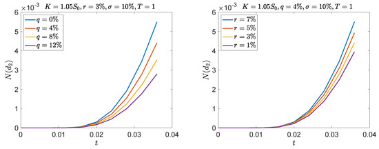
Figure 3.
Probability that a call option on S is in the money at the first eight monitoring dates. Daily monitoring (250 dates for a year maturity).
Table 2 shows some numerical examples. Three levels of moneyness are considered. In the first case, , the LSM provides good results even without any correction, but in the case large dividend yield: nevertheless, the distortion here is quite small and the price of the American option is much larger than its European counterpart and quite close to the benchmark. However, the correction of the LSM fixes this issue and delivers coherent results. In the other two levels of moneyness, when the option starts a little bit more out of the money, the LSM without correction heavily underprices the American call delivering also large standard errors.
Table 2.
Numerical results, Black–Scholes–Merton model. , , , 150 possible exercise dates per year. : initial price of the European call option computed with the Black–Scholes–Merton formula. : initial price of the American call option computed with the Cox–Ross–Rubinstein binomial tree (average of the price obtained with 250 and 251 steps). (): initial price of the American call option computed with the LSM not corrected (corrected) for the pitfalls previously described; the first six Laguerre polynomials are used for the regression: , with ; , standard errors obtained by 20 independent MC simulations. MC estimates that do not include the benchmark value within the confidence interval are denoted by .
When any of the corrections to the LSM is implemented instead, the results basically coincide with the ones derived in the binomial model of Cox et al. (1979), which, for the large number of the steps considered, can be assumed as a benchmark. Numerical imprecisions appear also when early exercise is never optimal () and, therefore, the price of the European option and of the American are roughly the same. In this case, the tiny difference between the two is much smaller than the confidence interval of the LSM’s estimates and such approach delivers unreliable results.
Completely analogous (and symmetric) results are obtained for out of the money put options, especially when the dividend yield q is low and the risk-free interest rate r is high. See, e.g., Carr and Chesney (1997); Detemple (2001) for a throughout discussion on the put-call symmetry for American-style options.
3. American Equity Options, Jump-Diffusion Model
In this Section, I propose a first variation of the standard Black–Scholes market. More specifically, I allow for stock price process to jump at random dates and with an idiosyncratic intensity. For the sake of simplicity, the risk-free interest rate is kept constant. The result is the well known jump-diffusion model first introduced by Merton (1976), which can be seen as the first generalization of the standard Black–Scholes–Merton model.
As in the previous section, Section 3.1 describes the theoretical aspects of the analysis, whereas Section 3.2 contains the related numerical examples.
3.1. Theoretical Framework: The Primary Assets and the Derivatives
Assume that the market is arbitrage free. Two assets are traded: the usual riskless bond and a risky asset S. To match some features of real market data like high peaks and heavy tails, it is convenient to relax the continuity hypothesis of the risky stock’s price and allow it to jump at random times. This introduces a new source risk in the market: The jump risk. Following the seminal work of Merton (1976) and as greatly explained by Glasserman (2003), I postulate that, since jumps are assumed to be independent of each other and of the stock’s level, the jump risk can be diversified away by investing in many difference stocks. Hence, the investors require no jump risk premium. This hypothesis being made, the risk-neutral measure becomes unique and derivatives on S can be priced uniquely.
Under , the price process of S solves
where is a jump process, s are i.i.d. positive random variables and is a Poisson process with intensity that counts how many jumps occurred before t included (with the convention ). As outlined before, , the s and N are assumed to be independent of each other. Jumps arrive at random instants and the waiting time before to consecutive jumps is exponentially distributed with parameter . Furthermore, it is convenient to assume that the jumps s are -lognormally distributed with mean a and volatility .
Under all of these assumptions and setting , the explicit solution of in Equation (8) is
and, conditioning on n jumps having occurred before t, namely, conditioning on ,
where Z is standard normal random variable independent of . It also holds true in distribution
with and . The deterministic drift of here is , strictly lower than in the standard model when .
The price at t of European and American derivatives within the present jump-diffusion model are still given by the risk-neutral expected values in Equations (3) and (4). For the European call, with and suppressing the argument of and , it holds
with , and
As usual, the pricing formula for a European put option can be retrieved by put-call parity.
The pricing of American options within the jump-diffusion model has to rely on numerical techniques instead, based on extensions of the celebrated Black–Scholes partial differential equation (see, e.g., Kinderlehrer and Stampacchia (2000) for a complete analysis on how to price American options through variational inequalities and Friedman (1982) for general solving schemes for PDEs and free boundary problems). Zhang (1997) provided an extremely useful characterization of a finite difference scheme to price American options in the jump-diffusion model.
3.2. Numerical Investigation
With the very same technique exploited to derive and starting from Equation (9), it can be shown that the risk-neutral probability that a call option on S is in the money at is
This probability is again increasing in r and decreasing in q, as Figure 4 shows. Nevertheless, as the drift of the underlying is now smaller due to the non negligible probability of a downward jump, this probability is slightly larger than the same one in the standard diffusive model.
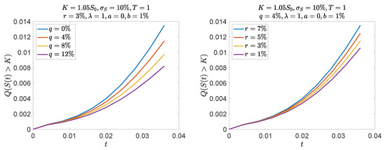
Figure 4.
Probability that a call option on S in jump-diffusion framework is in the money at the first eight monitoring dates. Daily monitoring (250 dates for a year maturity).
This implies a lower expected growth of S that translates into smaller call option prices, as it can be seen comparing Table 2 and Table 3 that share the same parameters.
Table 3.
Numerical results, jump-diffusion. , , , , , ; 150 possible exercise dates per year. : initial price of the European call option computed with Equation (10). : initial price of the American call option computed solving the free boundary problem by finite differences. (): initial price of the American call option computed with the LSM not corrected (corrected) for the pitfalls previously described; the regression involves the first six Laguerre polynomials for the values of the immediate exercise payoff; , standard errors obtained by 20 independent MC simulations. MC estimates that do not include the benchmark value within the confidence interval are denoted by .
As can be seen from the numerical examples in Table 3, the LSM works almost fine also at an intermediate level of out of moneyness, but when the dividend rate is too large.
This is coherent with the numerical figures of the previous section. Again, when the early exercise is almost never optimal, the price of the European option falls inside the confidence interval of the Monte Carlo estimate for the American price, making it not really reliable.
4. American Equity Options, Stochastic Interest Rates
In this section, I propose a second generalized market where the short-term risk free interest rate is stochastic. More specifically, I assume that the interest rate follows a mean-reverting stochastic process, as described first by the seminal work of Vasicek (1977). For the sake of simplicity, the volatilities of both the stock price process and of the locally risk-free interest rate are assumed to be constant. As in Section 2 and Section 3, Section 4.1 describes the theoretical aspects of the analysis, whereas Section 4.2 contains the related numerical examples.
4.1. Theoretical Framework: The Primary Assets and the Derivatives
Assume that the market is arbitrage-free. The locally risk-free interest rate r follows an Ornstein–Uhlenbeck process. The locally risk-free rate is capitalized through a bond whose price at t is . A zero-coupon bond is traded in market as well. It pays out 1 at maturity T and its price at t is labeled by . As in the previous Section, this markets involves two sources of uncertainty: The standard diffusive market risk and the interest rate one. Nevertheless, since the investor can hedge from both through S and the T-bond, the market is complete and all the derivatives can be uniquely priced. The explicit formula for the price of the zero-coupon bond can be found, for example, in Brigo and Mercurio (2007). Finally, a lognormal risky security S is traded. I allow for a non-zero correlation between the two processes. Under the risk-neutral measure , the two solve the following SDEs:
with . According to standard notation, the new parameters in Equation (13) represent: the volatility of the risky asset, the speed of mean-reversion of the short-term interest rate, its long-run mean, the volatility of the short-term interest rate and the correlation between the Brownian shocks on S and r. The explicit solution to the SDEs in Equation (13) is
As before, the contribution of the drift of S, , prevails over its volatility part . Therefore, the expected behaviour of the paths of S depends mostly on the drift.
The pricing formulas for European and American derivatives with maturity and payoff closely recall Equations (3) and (4):
For European call and put options, the pricing formulas depart slightly from the standard Black–Scholes–Merton ones as now the variability of the locally risk-free interest rate has to be accounted for. The full derivation of the modified formulas can be found in the Appendix of Battauz and Rotondi (2019). For the European call option, and it holds
with
whereas the related formula for the European put option can be retrieved by put-call parity.
The extension of the pricing to American options is less trivial. The variational inequality approach can be generalized including the new state variable r but it becomes quite tricky. On the contrary, the generalization of the binomial tree of Cox et al. (1979) is less involved: Battauz and Rotondi (2019) proposed a quadrinomial tree that models the joint evolution of S and r within a lattice structure. This allows for a relatively simple and fast evaluation of American claims.
Longstaff and Schwartz (2001) already allowed in their original work for a stochastic interest rate, which actually changes a little the LSM described in the previous Section. Nevertheless, the valuation algorithm suffers from the same drawbacks of the constant interest rate framework as the following subsection shows.
4.2. Numerical Investigation
Since the core of the LSM is unchanged, the drawback spotted out in the previous section might affect the pricing exercise also in this framework. The risk-neutral probability that the option is in the money is still pivotal. Going through the proof of Equation (15), it turns out that, in the present framework, the risk-neutral probability evaluated at that a call option is in the money at a given is
where is defined in Equation (16). At the first steps of the LSM, this probability is again extremely low if the option starts even a little bit out of the money.
Figure 5 shows that also when the short-term interest rate is stochastic, very few paths of a simulation are expected to be in the money at the first monitoring dates. Without the numerical correction proposed at the end of Section 2.1, the LSM is likely to provide again wrong estimates.
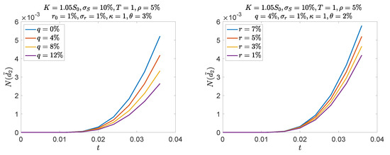
Figure 5.
Probability that a call option on S in a stochastic interest rate framework is in the money at the first eight monitoring dates. Daily monitoring (250 dates for a year maturity).
Table 4.
Numerical results, Vasicek model. , , , , , ; 150 possible exercise dates per year. : initial price of the European call option computed with Equation (15). : initial price of the American call option computed with the quadrinomial tree of Battauz and Rotondi (2019) (average of the price obtained with 150 and 151 steps). (): initial price of the American call option computed with the LSM not corrected (corrected) for the pitfalls previously described; the regression involves the first four Laguerre polynomials for the values of the immediate exercise payoff and the first four Laguerre polynomials for the current value of r; , standard errors obtained by 20 independent MC simulations. MC estimates that do not include the benchmark value within the confidence interval are denoted by .
First, it is interesting to notice that prices do not vary much when with respect to the ones obtained with a deterministic interest rate . This is due to the fact that, in the stochastic interest rate case, the long-run value is exactly ; therefore, r is simply expected to oscillate around in a symmetric (and thus not very relevant) way. Prices are a little bit higher in the stochastic rate framework to account for the variability in the interest rate itself. This variability is relevant when is significantly different from . When , r is expected to decrease towards : This implies a lower expected drift of S and a smaller call option’s price with respect to the standard case with a deterministic . The converse holds true when , thus delivering a larger call option’s price with respect to the standard model. If the pitfalls of the LSM are not corrected as proposed, the prices of the American call options fall constantly below their European counterpart. If the correction is made, instead, the LSM produces results that are comparable to the benchmark.
5. American Equity Options, Stochastic Volatility
Finally, in this section, I propose a third generalization of the standard Black–Scholes market. More specifically, I allow for the volatility of the stock price process to be stochastic while setting, for the sake of simplicity, the risk-free interest rate to be constant. The result is the celebrated model of stochastic volatility first introduced by the seminal work of Heston (1993).
As in the previous sections, Section 5.1 describes the theoretical aspects of the analysis, whereas Section 5.2 contains the related numerical examples.
5.1. Theoretical Framework: The Primary Assets and the Derivatives
Assume that the market is arbitrage-free. The instantaneous variance of the stock process S follows a Cox-Ingersoll-Ross (CIR henceforth) process, namely, a mean-reverting, non-negative12 stochastic process first introduced by Cox et al. (1985). In this setting, the market involves two state variables: the risky asset’s price and the volatility level. Consequently, there are two types of risks: the standard diffusive risk associated to S and the new volatility risk associated to . Since only the risky stock S and the riskless bond are traded, the market is not complete as the investor cannot hedge from the volatility risk. Therefore, the risk neutral measure is not unique. Nevertheless, uniqueness of contingent claims’ prices in this incomplete market is still attainable by making an assumption on the price of volatility risk. As proposed by Heston (1993), I assume that the price of volatility risk is proportional to the instantaneous volatility itself and I denote the constant of proportionality by , which becomes another exogenous parameter of the model. Thanks to this assumption, the risk-neutral measure is unique and the processes that drive the markets solve the following SDEs
with . According to standard notation, the new parameters in Equation (18) represent: the speed of mean-reversion on the volatility, its long-run mean, the volatility of the volatility process (the so called “vol of vol”), and the correlation between the Brownian shocks on S and . Although admits no explicit solution13, the one for in Equation (18) is
As before, the contribution of the drift of S, prevails over its diffusive part and it is still the main driver of its expected future behaviour.
The price at t of European and American options are still given by the risk-neutral expected values in Equation (3) and (4), where now the dynamics of S is shown by Equation (19).
For European options, the closed-form pricing formula are derived in the first section of Heston (1993). For the European call option, namely when the payoff function is , it holds at any
with
where i is the imaginary unit, Re the real part operator and, for ,
The analogous formula for the European put option can be retrieved by put-call parity.
The pricing of American option within this stochastic volatility framework is quite challenging. This is precisely one of the cases in which the LSM is of great help as, on the contrary, one can easily simulate the paths of Equation (18). The benchmark I will compare the performance of the modified LSM to is a finite difference approach to the free boundary problem for the American call option (see, e.g., Pascucci (2008) on this approach). The following numerical investigation focuses on the American call option in the Heston model; analogous results can be retrieved by the put–call symmetry for American options within the Heston model described by Battauz et al. (2014).
5.2. Numerical Investigation
By analogy with the standard Black–Scholes–Merton formula and as carefully described by Heston (1993), in Equation (20) represents the risk-neutral probability that an European call option on S closes in the money. As in the previous cases, this probability depends heavily on the drift of S, , and it is increasing with respect to the risk-free interest rate and decreasing with respect to the dividend yield.
Figure 6 provides a graphical illustration of this intuition. Notice that, as in the previous cases, at the first monitoring dates, very few paths are expected to be in the money if the option is even mildly out of the money at inception. As before, this worsens when the drift of the underlying becomes negative.
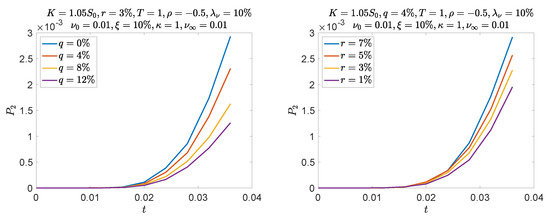
Figure 6.
Probability that a call option on S in within the Heston model is in the money at the first eight monitoring dates. Daily monitoring (250 dates for a year maturity).
Table 5 shows some numerical examples in the spirit of the previous sections. First, prices of the options are a little bit larger here with respect to the standard model due to the positive volatility risk premium. Then, the LSM fails in providing correct estimates in the very same cases of the standard model. Nevertheless, the correction is still effective.
Table 5.
Numerical results, Heston model. , , , , , , ; 150 possible exercise dates per year. : initial price of the European call option computed with Equation (20). : initial price of the American call option computed solving the free boundary problem by finite differences. (): initial price of the American call option computed with the LSM not corrected (corrected) for the pitfalls previously described; the regression involves the first four Laguerre polynomials for the values of the immediate exercise payoff and the first four Laguerre polynomials for the current value of ; , standard errors obtained by 20 independent MC simulations. MC estimates that do not include the benchmark value within the confidence interval are denoted by .
6. Conclusions
The Least Square Methods proposed by Longstaff and Schwartz (2001) is one of the most widely used algorithms to price American equity options. I quantified and corrected a sizeable bias that could arise if the regression exploited for the approximation of the continuation value of the option is ill-posed. I showed that this might happen when the option is even mildly out of the money at inception and when the underlying is not likely to go back into the in the money region. For American call options, this is likely to happen when the risk-free interest rate is low and the dividend yield is higher within the all the most commons financial market models.
Funding
This research received no external funding.
Acknowledgments
I thank Anna Battauz for insightful discussions and precious comments on the present work; all the remaining errors are my own.
Conflicts of Interest
The author declares no conflict of interest.
References
- Abramowitz, Milton, and Irene A. Stegun. 1970. Handbook of Mathematical Functions. Mineola: Dover Publications. [Google Scholar]
- Battauz, Anna, and Francesco Rotondi. 2019. American Options and Stochastic Interest Rates. Available online: http://didattica.unibocconi.it/mypage/index.php?IdUte=49395&idr=6877&lingua=ita (accessed on 21 March 2019).
- Battauz, Anna, Marzia De Donno, and Alessandro Sbuelz. 2014. The put-call symmetry for American options in the Heston stochastic volatility model. Mathematical Finance Letters 7: 1–8. [Google Scholar]
- Belomestny, Denis, Fabian Dickmann, and Tigran Nagapetyan. 2015. Pricing Bermudan options via multilevel approximation methods. SIAM Journal on Financial Mathematics 6: 448–66. [Google Scholar] [CrossRef][Green Version]
- Björk, Tomas. 2009. Arbitrage Theory in Continuous Time, 3rd ed. Hong Kong: Oxford Finance. [Google Scholar]
- Black, Fischer, and Myron Scholes. 1973. The pricing of options and corporate liabilities. Journal of Political Economy 81: 637–54. [Google Scholar] [CrossRef]
- Brigo, Damiano, and Fabio Mercurio. 2017. Interest Rate Models-Theory and Practice: With Smile, Inflation and Credit. Berlin: Springer Science & Business Media. [Google Scholar]
- Carr, Peter, and Marc Chesney. 1997. American Put Call Symmetry. Available online: https://pdfs.semanticscholar.org/fed1/b276f01b0ddb787cfcc9d0d2b8953fcd03dc.pdf (accessed on 21 March 2019).
- Carr, Peter, and Dilip Madan. 2001. Optimal positioning in derivative securities. Quantitative Finance 1: 19–77. [Google Scholar] [CrossRef]
- Clément, Emmanuelle, Damien Lamberton, and Philip Protter. 2002. An analysis of a least squared regression method for American option pricing. Finance and Stochastics 6: 449–71. [Google Scholar] [CrossRef]
- Cox, John C., Jonathan E. Ingersoll, and Stephen A. Ross. 1985. A theory of the term structure of interest rates. Econometrica 53: 385–407. [Google Scholar] [CrossRef]
- Cox, John C., Stephen A. Ross, and Mark Rubinstein. 1979. Option pricing: A simplified approach. Journal of Financial Economics 7: 229–63. [Google Scholar] [CrossRef]
- Detemple, Jerome. 2001. American options: Symmetry properties. In Handbooks in Mathematical Finance. Cambridge: Cambridge University Press, pp. 67–104. [Google Scholar]
- Detemple, Jerome. 2014. Optimal exercise for derivative securities. Annual Review of Financial Economics 6: 459–87. [Google Scholar] [CrossRef]
- Fabozzi, Frank J., Tommaso Paletta, and Radu Tunaru. 2017. An improved least squares Monte Carlo valuation method based on heteroscedasticity. European Journal of Operational Research 263: 698–706. [Google Scholar] [CrossRef]
- Friedman, Avner. 1982. Variational Principles and Free Boundary Problems, Pure and Applied Mathematics. Hoboken: Wiley. [Google Scholar]
- García, Diego. 2003. Convergence and biases of Monte Carlo estimates of American option prices using a parametric exercise rule. Journal of Economics and Control 27: 1855–79. [Google Scholar] [CrossRef]
- Glasserman, Paul. 2003. Monte Carlo Methods in Financial Engineering. Berlin: Springer. [Google Scholar]
- Heston, Steven L. 1993. A closed-form solution for options with stochastic volatility with applications to bond and currency options. The Review of Financial Studies 6: 327–43. [Google Scholar] [CrossRef]
- Kan, Kin Hung, and R. Mark Reesor. 2012. Bias reduction for pricing American options by least-squares Monte Carlo. Applied Mathematical Finance 19: 195–217. [Google Scholar] [CrossRef]
- Kinderlehrer, David, and Guido Stampacchia. 2000. An introduction to variational inequalities and their applications. Classics in Applied Mathematics. In Society for Industrial and Applied Mathematics. University City: SIAM, vol. 31. [Google Scholar]
- Longstaff, Francis A., and Eduardo S. Schwartz. 2001. Valuing American options by simulation: A simple least-square approach. The Review of Financial Studies 14: 113–47. [Google Scholar] [CrossRef]
- Merton, Robert C. 1976. Option pricing when underlying stock returns are discontinuous. Journal of Financial Economics 3: 125–44. [Google Scholar] [CrossRef]
- Merton, Robert C. 1973. Theory of rational option pricing. Bell Journal of Economics and Management Science 4: 141–83. [Google Scholar] [CrossRef]
- Pascucci, Andrea. 2008. Free boundary and optimal stopping problems for American Asian options. Finance and Stochastics 12: 21–41. [Google Scholar] [CrossRef]
- Revuz, Daniel, and Marc Yor. 2001. Continuous Martingales and Brownian Motion, 3rd ed. Berlin: Springer. [Google Scholar]
- Vasicek, Oldrich. 1977. An equilibrium characterization of the term structure. Journal of Financial Economics 5: 177–88. [Google Scholar] [CrossRef]
- Wooldridge, Jeffrey M. 2013. Introductory Econometrics: A Modern Approach, 5th ed. South Western: Cengage Learning. [Google Scholar]
- Zhang, Xiao Lan. 1997. Numerical analysis of American option pricing in a jump-diffusion model. Mathematics of Operations Research 22: 668–90. [Google Scholar] [CrossRef]
| 1 | See, e.g., the CBOE Market Statistics annual report released by the Chicago Board Options Exchange, the largest trading market for derivatives. In 2016, the overall dollar value of all the equity options traded at the CBOE was roughly equal to $66 billion with an average of 1.35 million equity options traded daily corresponding to 205 million call options and 135 million put through the year. |
| 2 | I advisedly allow for in order to possibly replicate also the current situation of the Eurozone where “risk-free” government bonds, such as German ones, display negative yield up to few years maturities. |
| 3 | Under these assumptions, the market is actually also complete; therefore, the risk-neutral measure is unique. |
| 4 | It holds true (see, e.g., Revuz and Yor (2001)) that and almost surely; as , . |
| 5 | denotes the positive part. The holder of an option will exercise it if and only if it delivers a positive payoff; if this is not the case, the option will not be exercised and its payoff is floored at zero. |
| 6 | If the payoff from the immediate exercise at of the option is zero, a rational investor would not exercise it and she would surely hold it on waiting for a positive payoff later on. |
| 7 | Notice that, if the conditional expectation of two random variables, , is an element of the space, since is an Hilbert space, can be represented as a linear combination of the elements of an orthonormal basis of the space. |
| 8 | See, e.g., Wooldridge (2013), Section 2.2, for a careful explanation of the linear regression model and of the related necessary assumptions for its unbiased and efficient estimation. |
| 9 | For all the possible choices of basis functions , it holds that ; see Chapter 22 of Abramowitz and Stegun (1970) for a comprehensive review of the basis functions of . |
| 10 | The same analysis can be carried out within any of the three extensions to the standard diffusive model: No relevant differences arise though. |
| 11 | I’m grateful to an anonymous referee for suggesting this extremely simple and effective econometric-based workaround. |
| 12 | With respect to the specification of in Equation (18), if the so-called Feller condition holds true, namely if , is also strictly positive almost surely. |
| 13 | As effectively explained in Subsection 3.4 of Glasserman (2003), a CIR process is not explicitly solvable; nevertheless, it can be shown that it is distributed, up to a scale factor, as a non-central chi-squared random variable. |


© 2019 by the author. Licensee MDPI, Basel, Switzerland. This article is an open access article distributed under the terms and conditions of the Creative Commons Attribution (CC BY) license (http://creativecommons.org/licenses/by/4.0/).