Article

Market-Risk Optimization among the Developed and Emerging Markets with CVaR Measure and Copula Simulation

by
Nader Trabelsi
1,2,* and
Aviral Kumar Tiwari
3,4
1
Department of Finance and Investment, Imam Muhammad Bin Saud Islamic University, Riyadh 5701, Saudi Arabia
2
LARTIGE, University of Kairouan, Dar El Amen Kairouan 3100, Tunisia
3
Finance Law & Control, Montpellier Business School, 34000 Montpellier, France
4
Rajagiri Business School, Rajagiri Valley Campus, Kochi 682 039, India
*
Author to whom correspondence should be addressed.
Risks 2019, 7(3), 78; https://doi.org/10.3390/risks7030078
Submission received: 3 May 2019 / Revised: 16 June 2019 / Accepted: 26 June 2019 / Published: 7 July 2019

Abstract

:
In this paper, the generalized Pareto distribution (GPD) copula approach is utilized to solve the conditional value-at-risk (CVaR) portfolio problem. Particularly, this approach used (i) copula to model the complete linear and non-linear correlation dependence structure, (ii) Pareto tails to capture the estimates of the parametric Pareto lower tail, the non-parametric kernel-smoothed interior and the parametric Pareto upper tail and (iii) Value-at-Risk (VaR) to quantify risk measure. The simulated sample covers the G7, BRICS (association of Brazil, Russia, India, China and South Africa) and 14 popular emerging stock-market returns for the period between 1997 and 2018. Our results suggest that the efficient frontier with the minimizing CVaR measure and simulated copula returns combined outperforms the risk/return of domestic portfolios, such as the US stock market. This result improves international diversification at the global level. We also show that the Gaussian and t-copula simulated returns give very similar but not identical results. Furthermore, the copula simulation provides more accurate market-risk estimates than historical simulation. Finally, the results support the notion that G7 countries can provide an important opportunity for diversification. These results are important to investors and policymakers.

1. Introduction

Since Markowitz published his seminal paper in 1952 (Markowitz 1952), the mean-variance (MV) optimization framework has been an effective way to measure and compare the risk/return trade-off among various portfolios. However, despite its success, this approach has many limitations, which include, but are not limited to, the abnormal distributed returns in recent times. The copula is a very useful tool for dealing with non-standard distribution (see Clemente and Romano 2004; Rockafellar and Uryasev 2000; among others). Furthermore, it has become increasingly popular for modelling the dependence structure of financial risks. On the other hand, the number and intensity of crises (including, for example, the terrorist attacks on 11 September 2001, the Iraq invasion in 2003, the 2007–2009 global financial crisis sparked by US subprime market failures, the 2009–2013 European sovereign-debt crises etc.) that have occurred in the past decades have made the measurement of market risk a primary concern of regulators and academics.
In the literature, tail-related risk measures, such as the VaR and conditional value-at-risk (CVaR), have become the most widely used measures of market risk (see Cherubini et al. 2004; Komang 2013; Rockafellar and Uryasev 2002; among others). Our work is thus broadly related to these studies. Our objective is to discuss for US investors the adequacy of a global stock portfolio invested in three categories of markets: the G7, BRICS and the most popular emerging countries. Beyond the classical portfolio characteristics, we consider additional portfolio characteristics such as CVaR and copula theory. In particular, we apply a Gaussian copula and the Student’s t-copula model to create a joint distribution of returns and then use VaR and CVaR measures for portfolio selection. Finally, the VaR and CVaR portfolios produced by the copula simulation are compared to those produced from the historical record.
To that end, extreme value theory (EVT) is applied to estimate the tails of abnormally distributed marginal density functions (see Embrechts et al. 1997; Hotta et al. 2008; among others). The distribution of each return series is fitted semi-parametrically. A benefit of this approach is that it requires estimating the lower and upper tails parametrically, while the interior is estimated by the non-parametric, kernel-smoothed interior method. Our data cover the G7 group (the United States (US), Canada, France, the United Kingdom (UK), Italy, Japan and Germany), the BRICS group (Brazil (Bra), Russia (RS), China, India, South Africa (SA)) and 14 popular emerging stock-market returns other than the BRICS group (Chile, Mexico, Peru, Czech Republic (Czech.R), Greece, Hungary, Poland, United Arab Emirates (UAE), Indonesia, Korea, Malaysia, Philippines, Taiwan and Thailand). The sample data recorded during the period between 31 March 1997 and 30 April 2018 were used to compose the global portfolio.
The empirical results show that the historical simulation model produced aggressive VaR and CVaR estimates compared to those provided by copula simulations. This result thus makes VaR and copulas attractive and efficient tools for portfolio selection, as they can capture the extreme events that characterize our recent economic conditions. Furthermore, we find that US investors can find a minimum CVaR portfolio in developed economies rather than in many other developing or emerging stock markets.

2. Literature Review

Portfolio selection is peculiarly susceptible to model the risk and the profit/loss distribution density. Errors in describing or estimating the probability distribution can profoundly affect investor’s welfare. In portfolio analysis, an incorrect model risk can lead to an incorrect implementation of a diversification and hedging strategies.
Since its adoption by Basel II in 1996, VaR has become the most widely used measure of financial risk compared to the standard deviation. A back-testing procedure is used to count VaR ‘violations’, i.e., the number of times the actual return fell below the VaR forecast. However, VaR fails to satisfy mathematical principles characterizing coherent risk measures (Chen 2018). In addition to ignoring losses beyond a designated threshold, VaR lacks subadditivity. In financial regulatory (i.e., Basel II and III), expected shortfall and expectiles are now used by the most financial institutions to offset the weaknesses of VaR in assessing credit risk (for a detailed discussion of computation and forecasting methods of VaR and CVaR measures as Basel II and III accords, please see Nolde and Ziegel (2017); Bellini et al. (2017); Chen (2018); among others).
CVaR/VaR are also used in the area of portfolio optimization for a relatively long period of time with many solution methods, including decomposition of the model, linear approximation, heuristic algorithms, etc. (for more details see Zhang 2016). According to some sources (e.g., Rockafellar and Uryasev 2000, 2002; Krokhmal et al. 2003; Alexander et al. 2006; Cox et al. 2009; Najafi and Mushakhian 2015; among others), CVaR is used as an alternative measure that does quantify the losses that might be encountered in the tail. Rockafellar and Uryasev (2000, 2002); Krokhmal et al. (2003) are the pioneers in developing efficient algorithms of portfolio allocation that take in account CVaR as a risk measure to be minimized in the objective function. This approach corresponds to the Markowitz Mean-Variance model (MV model). While compared to VaR optimization, the main benefit of a CVaR optimization is that it can be implemented as a linear programming problem (Alexander et al. 2006). Cox et al. (2009) extended the Krokhmal, Palmquist, and Uryasev’s approach by using CVaR-like constraints in the traditional portfolio optimization problem to reshape either the left or right tail of a portfolio return distribution. Najafi and Mushakhian (2015) suggested a multi-period portfolio selection model with CVaR at a given confidence level α. In line with these extensions, Cao (2015) presented a CVaR portfolio model based on a combination of capital gains rate not assuming a normal distribution, with the Mean Absolute Deviation (MAD) model as a constraint, realized volatility measure limit, spend a convex utility function as a constraint, indicating risk asset transaction costs. Li and Xu (2013) developed the mean-CVaR portfolio selection problem in a continuous-time dynamic setting. When expected return is replaced by expected utility, the maximization of a utility function that balances CVaR against return is also studied in a continuous-time dynamic setting by Gandy (2005) and Zheng (2009). Note that the VaR/CVaR risk measures can be also found in other literature focused on systemic risk such as Acharya et al. (2009); Chen et al. (2013) and Adrian and Brunnermeier (2016).
In addition to the violation of the standard deviation as a risk measure, there are more discussions on the bias of the linear correlation between assets. In financial literature, to circumvent this problem an alternative approach has been suggested based on Copula theory. This theory takes mainly in account the presence of linear and non-linear interdependence between assets. More importantly, CVaR can be readily estimated in capturing by copula the non-linear interdependence at the tails between the marginal returns. He and Gong (2009) constructed a copula-CVaR model for credit risks of listed company on Chinese security market and this model can exactly measure the coupled risks in financial market. Huang et al. (2009), Chen and Tu (2013) and Boubaker and Sghaier (2013) used the conditional Copula Generalized Autoregressive Conditional Heteroskedasticity (GARCH) model to describe the financial assets joint distribution included in portfolio. More recently, Nikusokhan (2018) employed the CVaR Glosten-Jagannathan-Runkle (GJR) Copula method and the emerging market data for portfolio risk identification and portfolio optimization. The empirical evidence suggests that the performance of the GJR-Copula-CVaR method is relatively more accurate and more flexible than other common methods of optimization. Sahamkhadam et al. (2018) used GARCH-EVT-copula and Auto-Regressive-Moving-Average (ARMA)-GARCH-EVT-copula models to perform out-of-sample forecasts and simulate one-day-ahead returns for 10 stock indexes. They constructed optimal portfolios based on the global minimum variance (GMV), minimum conditional value-at-risk (Min-CVaR) and certainty equivalence tangency (CET) criteria, and modeled the dependence structure between stock market returns by employing elliptical (Student-t and Gaussian) and Archimedean (Clayton, Frank and Gumbel) copulas. Their main finding is that the CET portfolio, based on ARMA-GARCH-EVT-copula forecasts, outperforms the benchmark portfolio based on historical returns. Moreover, the regression analyses show that GARCH-EVT forecasting models, which use Gaussian or Student-t copulas, are best at reducing the portfolio risk. Fernando et al. (2017) mixed Archimedean copula function and the CVaR minimization model to obtain efficient portfolios. Using data from the S&P500 stocks from 1990 to 2015, their empirical analysis shows that the Mixed Copula-CVaR approach generates portfolios with better downside risk statistics for any rebalancing period and it is more profitable than the Gaussian Copula-CVaR and the 1/N portfolios for daily and weekly rebalancing.
Beyond the existing literature, our main contribution is in combining the Generalized Pareto distribution copula approach and VaR/CVaR risk measures to find an empirical evidence of efficient portfolios (i.e., along the efficient frontiers) using data of many developed and developing or emerging stock markets.

3. Methodology

3.1. Generalized Pareto Distribution Copula Approach

It has been known since the work of Sklar (1959) that a joint distribution function H with continuous marginal distributions F and G can be characterized by a unique copula function C, such that, for all x, y in R ¯ ,   H ( x , y ) = C ( F ( x ) , G ( y ) ) . Many multivariate models for dependence can be generated by parametric families of copulas. In this study, two types of copulas are proposed: the Gaussian copula and the t-copula (i.e., the elliptical copula family). The Gaussian copula is formally defined as:
C ( u 1 , u n ; Λ ) = ϕ k ( ϕ 1 ( u 1 ) , ,   ϕ 1 ( u n ) ; Λ ) .
The copula function is defined by the standard multivariate normal distribution ( ϕ k ) and the linear correlation matrix ( Λ ) . This approach has been lately heavily criticized by academics and practitioners because it fails to capture dependence in the tail of distributions. This approach has, indeed, a zero coefficient for tail dependence, which means that events occur independently far enough in the tails of the joint distribution. Therefore, the use of another copula is highly recommended when considering extreme events. We propose the use of the t-copula because it presents symmetric lower and upper tail dependence coefficients.
The t-copula is closely related to the Gaussian copula with CDF:
C n ψ ( u ; Ω ψ ; v ) = ψ n ( ψ 1 ( u 1 , v ) , , ψ 1 ( u n ; v ) ; Ω ψ , v ) ,
where ψ n denotes the CDF of an n-variate Student’s t distribution with correlation Ω ψ , the degree of freedom parameters v > 2 and ψ 1 is the inverse of the CDF for the univariate Student’s t distribution with mean zero and the dispersion parameter is equal to 1.
For the t-copula, it is useful to fit the distribution of returns of each stock-index series using a piecewise distribution that is semi-parametric with generalized Pareto tails to model the tail behavior by means of the generalized Pareto distribution (GPD) approach. The Pareto tails capture the estimates of the parametric Pareto lower tail, the non-parametric kernel-smoothed interior and the parametric Pareto upper tail.
According to EVT, GPDs can be applied to model the tail behavior of returns in financial series exceeding the high thresholds x− λ . As shown by Scarrott and MacDonald (2012), the GPD is parameterized by scale and shape parameters σ λ > 0 and θ and can equivalently be specified in terms of exceedances x > λ as:
G θ ( x \ λ ,   σ λ ) = { 1 [ 1 + θ ( x λ σ λ ) ] + 1 θ   f o r   θ 0 1 [ e x λ σ λ ] +   f o r   θ = 0 ,
where y + = max ( y , 0 ) . When θ < 0 , there is an upper end point, so λ < x < λ σ λ θ (for more details, see Scarrott and MacDonald 2012).

3.2. Portfolio Optimization

We used VaR and CVaR measures to quantify the US investor’s risk exposure. In this case, VaR represents maximum potential loss l in the value of a portfolio with a given probability ‘X’ over a specified horizon. For the given confidence level α ( 0 , 1 ) , the VaR of a portfolio is then given by the smallest number l such that the probability that the loss L f ( w , r ) exceeds l is no greater than ( 1 α ) (Demarta and McNeil 2005). Hence, V a R α = i n f { l : P ( L < l ) l α } = i n f { : F l α } , where (w, r) denote the weights of the portfolio and the expected return of each stock market, respectively.
CVaR is a supplement or an alternative to VaR. It is also another percentile risk measure. For continuous distributions, CVaR is defined as the conditional expected loss under the condition that it exceeds VaR. Following Rockafellar and Uryasev (2000, 2002), the C V a R ( α ) of the loss associated with any w, it is found that
C V a R ( α ) = l + 1 1 α m a x { ( f ( w , r ) l ) } p ( r ) d r   .
The problem of minimizing the CVaR can thus be formulated as follows:
m i n i m i z e   C V a R ( α ) ,
S u b j e c t   t o   i = 1 n w i = 1 ,
w T E ( r ) r ,
where Equation (6) is the weight constrain condition, Equation (7) the expected return of the portfolio and p(r) is the joint distribution of the uncertain return of stocks exceeding a certain amount r .
In this work, the portfolio optimization was carried out with the minimization of CVaR subject to a constraint on expected return. A big advantage of CVaR over VaR in that context is the preservation of convexity. In this case the feasibility set satisfying Equations (6) and (7) is a convex region, due to linearity in constraints.

4. Results and Interpretations

Figure 1 shows plots of the distribution probabilities produced with the returns of two arbitrary markets (i.e., Brazil and Italy). It is important to note in this figure that the Pareto-distribution probability fits the data better than is the case with any other method, such as the normal distribution. In particular, we can show that the returns of the Brazilian and Italian stock indexes have a heavy left tail, which corresponds to the Pareto tail distribution with negative shape parameters.
Modelling the correlation structures of economic variables is also an important part of managing market risk. The easiest method is to use historical returns in this modelling. Such a procedure assumes the normal distribution of the returns. Figure 2 depicts the scatterplots of the pairwise linear correlation matrices between each pair of countries from the same set of observations (the results for BRICS are integrated into emerging markets) and corresponding distribution. The diagonal line is converted to display the distribution of historical returns.
The pairwise correlation between the two stocks is a value between −1 and 1 that indicates how likely the two stock markets are to move in the same direction. Not surprisingly, there is a significant positive correlation between the considered countries, with the exception of the US stock market with other markets (including the G7, BRICS and the most popular emerging countries), which have a low correlation. Additionally, the UAE and China also have a weak and negative correlation with most emerging countries. Thus, for US investors, a diversified portfolio that includes foreign equities optimizes the diversification risk/return rule. In other terms, this result may improve diversification at the global level. Indeed, despite its volatility profile, the emerging market offers diversification to US investors (see Ted 2016). Nevertheless, it is essential to note that the correlation estimations in Figure 2 have to be considered with great caution because, while they measure the linear dependence, other types of dependences (e.g., tail dependence) may not be captured. To alleviate this problem, we used a copula approach.
Although the calibration of the linear correlation matrix of a Gaussian copula is straightforward, the calibration of a t-copula is not. For this reason, we transformed t-centered returns to uniform variates by the piecewise, semi-parametric CDFs derived above (Note that the transformed dataset and corresponding distribution are available upon request).
The transformed marginal distribution, which was modelled on the basis of GDP, was then used to fit the Gaussian and t-copulas.
Figure 3 presents an accurate and interpretable characterization of the local dependence of the Gaussian and t-copula by means of a red/blue surface plot (Please see Appendix A for more details on elliptical copula parameters). This makes the interpretation much easier. As may be seen from Panels A and B, that the Gaussian and t-copula give very similar results. Moreover, the dependence structure among the US and considered stock markets is somewhat different. This dependence-structure distinction plays an important role in portfolio construction. More specifically, there is a blue color (i.e., low dependence) between the US and the most popular emerging stock markets; that is, there is low tail dependence among these markets. Likewise, a low tail dependence is also shown for the UAE and China with the rest of the most popular emerging markets. For BRICS countries, the blue color is also related to Russia and China. In the case of G7 countries, however, the blue color is essentially associated with Japan’s stock market. The tail dependence of other co-developed countries is mainly between yellow and red. These findings are not shown by the linear relationship. It is important to note that there is a greater non-linear and tail-dependence structure between financial markets over the past decade. The elliptical copula thus confirms its superiority (i.e., red color or high coefficients) to best fit this dependence structure, mainly among G7 as well as Eastern European stock markets (i.e., Czech.R, Hungary and Poland).
The Pareto-copula coefficients allow for estimating the new pricewise correlation matrices. Table 1 presents the GPD parameters (shape and scale) at the upper and lower tails for each individual country.
Figure 4 and Figure 5 depict scatterplot correlation matrices using Gaussian and t-copula simulated returns. Judging from the results in Figure 4 and Figure 5, it would appear that the novel estimated correlation matrices, including copula simulations (i.e., Gaussian and t-copula), are quite similar but not identical to the linear correlation matrices reported in Figure 2 (The average value of pairwise correlations using Gaussian and t-copula simulations are available upon request). The efficient frontier is used as a means of determining the desired portfolio of risky securities, each having an expected mean CVaR and a pairwise correlation matrix, among the securities’ returns comprising the portfolio. The efficient frontier can be generated for the risky portfolio that provides the maximum return and the minimum CVaR.
Figure 6 shows the efficient-frontier graphs using Gaussian (Panel A) and t-copula (Panel B) estimations for various sets of observations. We assume equally weighted portfolios and α = 99 % as a level for VaR and CVaR computation. In this figure, the dominance of the expected return of investment portfolios that included emerging markets was obvious (i.e., compared to domestic portfolios). This agrees with previous studies that support the performance of an investment in emerging markets (e.g., Aloui et al. 2011; Goetzmann et al. 2005; Hallinan 2011; among others). Additionally, one can observe the dominance of the minimum risk of portfolios that included only developed markets. On the other hand, there is no major difference between the efficient frontiers generated by the Gaussian and t-copula approaches.
This result can also be seen in Table 2, following the structures of optimal portfolios in terms of VaR and CoVaR measures. More precisely, the portfolios’ VaR and CVaR risks formed by simulating copulas were quite different, but with the minimum t-copula risk being superior to that of the Gaussian copula. This is due to the fact that the Gaussian copula and the t-copula come from the same family. However, this agreement between the two copulas should not mislead one into concluding that a copula from the same family will produce the same result. The obtained results depend on the characteristics of the dataset. On the other hand, Table 2 supports the conclusion that developed stock markets are a more effective tool in reducing portfolio risks than are many emerging stock markets. When extreme market events are taken into account, however, the emerging markets are more volatile.
Referring again to Table 2, it may be seen that the structures of the optimum portfolio given by the multivariate normal distribution are significantly different from those of the optimum portfolios created by simulating copulas. This kind of information may be of interest to the risk manager who wishes to formulate a hedging plan (e.g., derivatives) against potential losses.

5. Conclusions

This paper combines the CVaR and copula approaches for market-risk measurement of portfolios among three sets of stock markets, including the advanced nations that make up the G7 and BRICS and the most popular emerging stock markets. The empirical results show that the historical simulation model produced aggressive VaR and CVaR estimates compared to those provided by copula simulations. This result thus demonstrates that VaR and copulas are attractive and efficient tools for portfolio selection, as they can capture the extreme events that characterize our recent economic conditions. Furthermore, we find that US investors can find a minimum CVaR portfolio in developed economies rather than in many other developing or emerging stock markets.
Considering the literature of portfolio selection, our results also showed a difference between the multivariate normal distribution and copula simulation. Precisely, the copula method was superior than multivariate normal distribution, in describing the efficient frontier. Thus, developing a consistent methodology to construct an efficient frontier based on copula and CVaR measures, as we did in this paper, could be viewed as an incremental contribution to the literature in portfolio selection.
Finally, all these results are important to portfolio managers who are looking for adequate methods to estimate risk premiums, explicitly recognize extreme risks, to formulate a hedging plan, and to control gains rate fluctuations or risks.
However, it is important to note that Gaussian and t-copulas derived from elliptical probability distributions retain their underlying families’ essential characteristic of symmetry. In technical terms, this means that these copulas can handle differences in the even-numbered moments of a distribution, especially variance and kurtosis, but not skewness. To circumvent this problem, we suggest further research on the use of copulas that allow for the modelling of different tail dependences, such as the Archimedean (McNeil and Nešlehová 2009) and vine copulas (Bedford and Cooke 2002).

Author Contributions

The first author collected the data. Both authors contributed to the drafting of all sections of the paper.

Funding

This research received no external funding.

Conflicts of Interest

The authors declare no conflict of interest.

Appendix A. Elliptical Copula Parameters

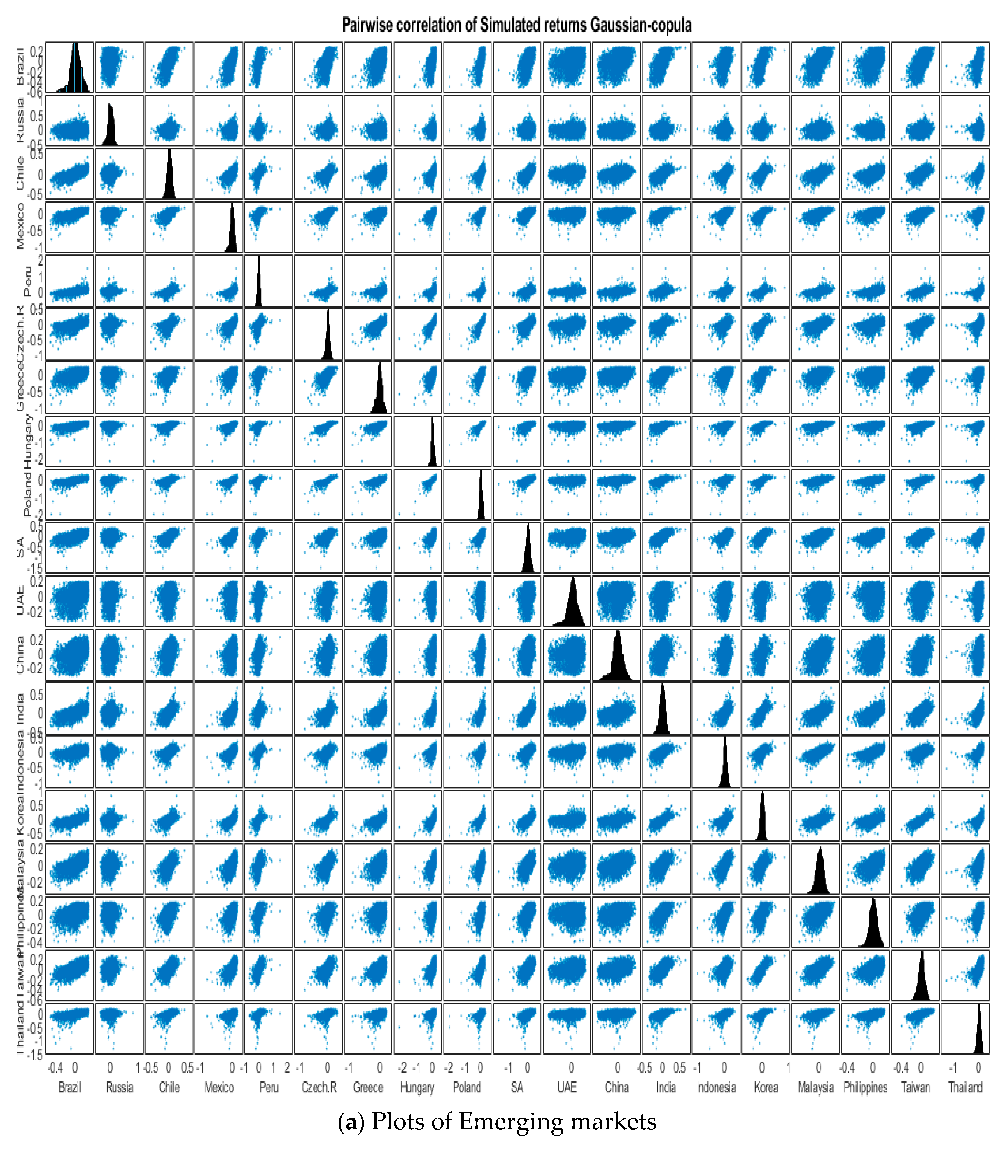
The bivariate Gaussian copula (N)—it has no tail dependence, hence τ U = τ L = 0. Therefore, modeling the dependence structure of the series by a Gaussian (normal) copula is consistent with the estimation of this dependence by the linear correlation coefficient such that 1 < ρ < 1 . The copula density is given by (see e.g., Cherubini et al. (2004))
C N ( u , v | ρ ) = Φ 1 ( u ) Φ 1 ( v ) 1 2 π 1 ρ 2 · e x p { ( r 2 2 ρ r s + s 2 ) 2 ( 1 ρ 2 ) }   drds ,  
where Φ ( · ) represents the univariate standard normal distribution function with correlation ρ ( 1 ,   1 ) .
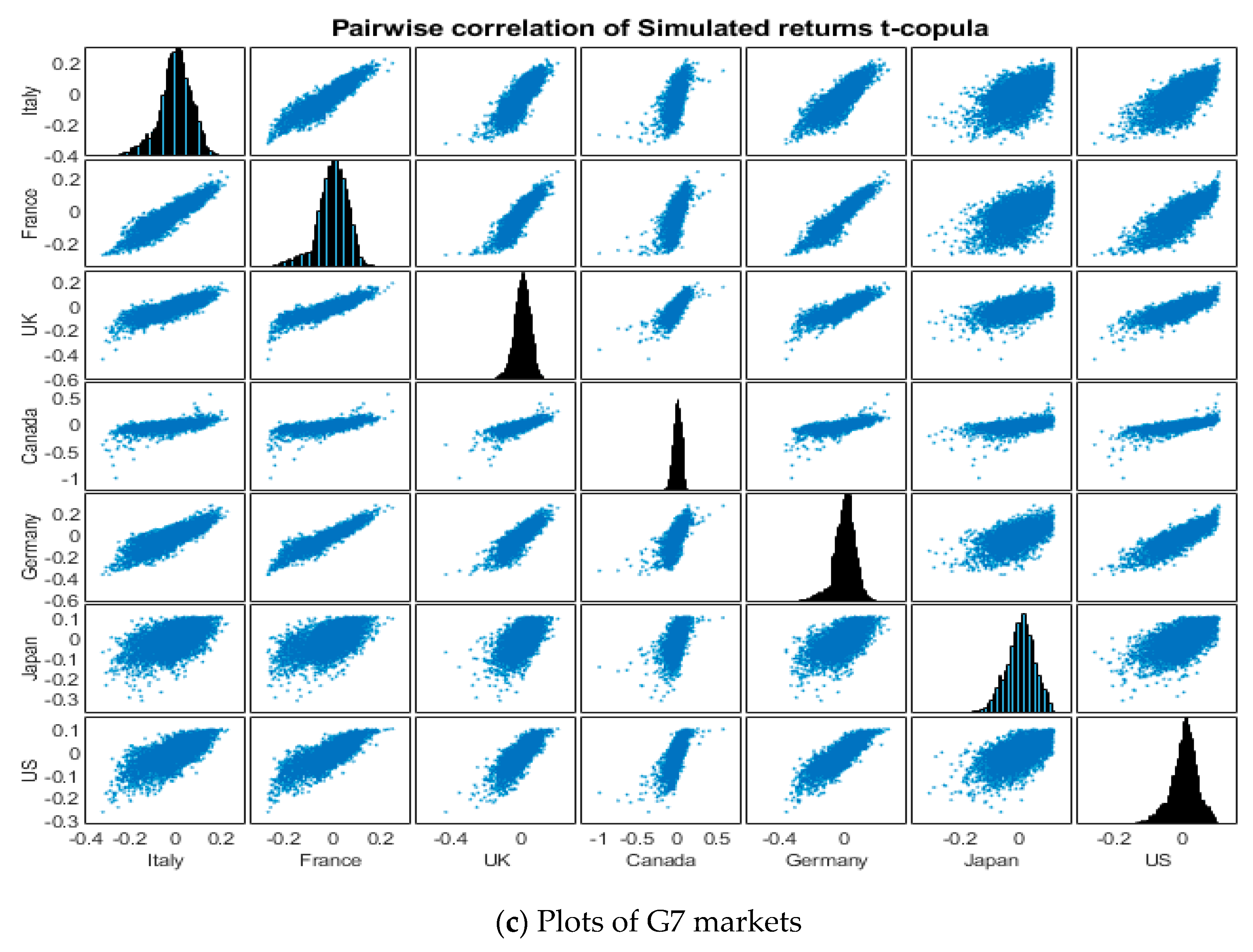
The t-copula—it also has a correlation coefficient such that 1 < ρ < 1 however, it shows some tail dependence. Specifically, it has symmetric tail dependence. It may be expressed as follows (see e.g., Cherubini et al. (2004)):
C S T ( u , v | ρ , ϑ ) = t ϑ 1 ( u ) t ϑ 1 ( v ) 1 2 π 1 ρ 2 · e x p { ( r 2 2 ρ r s + s 2 ) 2 ( 1 ρ 2 ) }   drds ,  
where t ϑ   ( · ) is a univariate Student-t distribution function with ϑ + 1 degrees of freedom and ρ ( 1 ,   1 ) . The symmetric tail dependence is τ U = τ L = 2 t ϑ + 1   ( ϑ + 1 1 ρ / 1 + ρ ) > 0 . As the t-copula allows for symmetric non-zero dependence in the tails and it represents a generalization of the Gaussian-copula.
Table A1. Description parameters of Copula.
FamilyParameters
Upper Tail DependenceLower Tail Dependence
Gaussian-copula τ U = 0 τ L = 0
t-copula τ U = 2 t ϑ + 1   ( ϑ + 1 1 ρ / 1 + ρ ) τ L = 2 t ϑ + 1   ( ϑ + 1 1 ρ / 1 + ρ )

References

  1. Acharya, Viral V., Lasse H. Pedersen, Thomas Philippon, and Matthew Richardson. 2009. Regulating Systemic Risk, Restoring Financial Stability: How to Repair a Failed System. Hoboken: Wiley, pp. 283–304. [Google Scholar]
  2. Adrian, Tobias, and Markus K. Brunnermeier. 2016. CoVaR. American Economic Review 106: 1705–41. [Google Scholar] [CrossRef]
  3. Alexander Siddharth, Coleman Thomas F., and Yuying Li. 2006. Minimizing CVaR and VaR for a Portfolio of Derivatives. Journal of Banking & Finance 30: 583–605. [Google Scholar]
  4. Aloui, Riadh, Duc Khuong Nguyen, and Mohamed Ben Aïssa. 2011. Global financial crisis, extreme interdependences, and contagion effects: The role of economic structure? Journal of Banking & Finance 35: 130–41. [Google Scholar]
  5. Bedford, Tim, and Roger M. Cooke. 2002. Vines—A new graphical model for dependent random variables. Annals of Statistics 30: 1031–68. [Google Scholar] [CrossRef]
  6. Bellini, Fabio, Klar Bernhard, and Müller Alfred. 2017. Expectiles, Omega ratios, and stochastic ordering. In Methodology and Computing in Applied Probability. Berlin: Springer. [Google Scholar]
  7. Boubaker, Heni, and Nadia Sghaier. 2013. Portfolio Optimization in the Presence of Dependent Financial Returns with Long Memory: A Copula Based Approach. Journal of Banking & Finance 37: 361–77. [Google Scholar]
  8. Cao, Jinsheng. 2015. Portfolio Optimization Model Based on CVaR Programming and Limits of MAD. Paper presented at the International Conference on Education Technology, Management and Humanities Science (ETMHS), Xi’an, China, 21–22 March. [Google Scholar]
  9. Chen, James Ming. 2018. On Exactitude in Financial Regulation: Value-at-Risk, Expected Shortfall, and Expectiles. Risks 6: 61. [Google Scholar] [CrossRef]
  10. Chen, Yi-Hsuan, and Anthony Tu. 2013. Estimating Hedged Portfolio Value-at-Risk Using the Conditional Copula: An Illustration of Model Risk. International Review of Economics & Finance 27: 514–28. [Google Scholar]
  11. Chen, F., X. Chen, Z. Sun, T. Yu, and M. Zhong. 2013. Systemic risk, financial crisis, and credit risk insurance. Financial Review 48: 417–42. [Google Scholar] [CrossRef]
  12. Cherubini, Umberto, Elisa Luciano, and Walter Vecchiato. 2004. Copula Methods in Finance. New York: John Wiley & Sons. [Google Scholar]
  13. Clemente, Annalisa Di, and Claudio Romano. 2004. Measuring and optimizing portfolio credit risk: A copula-based approach. Economic Notes by Banca Monte dei Paschi di Siena SpA 33: 325–57. [Google Scholar] [CrossRef]
  14. Cox, Samuel H., Yijia Lin, Ruilin Tian, and Luis Zuluaga. 2009. Portfolio Risk Management with CVaR-Like Constraints. North American Actuarial Journal 14: 86–106. [Google Scholar] [CrossRef]
  15. Demarta, Stefano, and Alexander J. McNeil. 2005. The t-copula and related copulas. International Statistical Review 73: 111–29. [Google Scholar] [CrossRef]
  16. Embrechts, Paul, Claudia Klüppelberg, and Thomas Mikosch. 1997. Modelling Extremal Events for Insurance and Finance. Berlin: Springer. [Google Scholar]
  17. Fernando, A. B. Sabino da Silva, Flávio A. Ziegelmann, and Cristina Tessari. 2017. Robust Portfolio Optimization with Multivariate Copulas: A Worst-Case Cvar Approach. Working Paper, unpublished. [Google Scholar] [CrossRef]
  18. Gandy, Robin. 2005. Portfolio Optimization with Risk Constraints. Ph.D. dissertation, Universität ULM, Denmark. Available online: http://vts.uni-ulm.de/docs/2005/5427/vts5427.pdf (accessed on 13 December 2005).
  19. Goetzmann, William, Lingfing Li, and K. Geert Rouwenhorst. 2005. Long-term global market correlations. Journal of Business 78: 1–38. [Google Scholar] [CrossRef]
  20. Hallinan, Kelly. 2011. The Role of Emerging Market in Investment Portfolios. Honours Scholar thesis. Available online: http://digitalcommons.uconn.edu/srhonors_theses/200 (accessed on 5 August 2011).
  21. He, Xubiao, and Pu Gong. 2009. Measuring the coupled risks: A copula-based CVaR model. Journal of Computational and Applied Mathematics 223: 1066–80. [Google Scholar] [CrossRef]
  22. Hotta, Luiz Koodi, Edimilson C. Lucas, and Helder P. Palaro. 2008. Estimation of VaR using copula and extreme value theory. Multinational Finance Journal 12: 205–21. [Google Scholar] [CrossRef]
  23. Huang, Jen Jsung, Jung Kuo, Hueimei Liang, and Wei-Fu Lin. 2009. Estimating Value at Risk of Portfolio by Conditional Copula-GARCH Method. Insurance 45: 315–24. [Google Scholar] [CrossRef]
  24. Komang, Dharmawan. 2013. Measuring and Optimizing Conditional Value at Risk Using Copula Simulation. Paper presented at South East Asian Conference on Mathematics and Its Application (SEACMA 2013), Surabaya, Indonesia, 11–15 November. [Google Scholar]
  25. Krokhmal, Pavlo, Jonas Palquist, and Stanislav Uryasev. 2003. Portfolio Optimization with Conditional Value-at-Risk Objective and Constraints. Journal of Risk 4. [Google Scholar] [CrossRef]
  26. Li, Jing, and Mingxin Xu. 2013. Optimal Dynamic Portfolio with Mean-CVaR Criterion. Risks 1: 119–47. [Google Scholar] [CrossRef]
  27. Markowitz, H. 1952. Portfolio selection. Journal of Finance 7: 77–91. [Google Scholar]
  28. McNeil, Alexander J., and Johanna Nešlehová. 2009. Multivariate Archimedean copulas, $d$-monotone functions and $l_1$-norm symmetric distributions. Annals of Statistics 37: 3059–97. [Google Scholar] [CrossRef]
  29. Najafi, Amir Abbas, and Siamak Mushakhian. 2015. Multi-stage stochastic mean-semivariance-CVaR Optimization under Transaction Costs. Applied Mathematics and Computation 256: 445–58. [Google Scholar] [CrossRef]
  30. Nikusokhan, Moien. 2018. GJR-Copula-CVaR Model for Portfolio Optimization: Evidence for Emerging Stock Markets. Iranian Economic Review 22: 990–1015. [Google Scholar]
  31. Natalia, Nolde, and Johanna F. Ziegel. 2017. Elicitability and backtesting: Perspectives for banking regulation. The Annals of Applied Statistics 11: 1833–74. [Google Scholar]
  32. Rockafellar, R. Tyrrel, and Stanilav Uryasev. 2000. Optimization of conditional value-at-risk. Journal of Risk 2: 21–41. [Google Scholar] [CrossRef] [Green Version]
  33. Rockafellar, R. Tyrrel, and Stanislav Uryasev. 2002. Conditional value-at-risk for general loss distributions. Journal of Banking and Finance 26: 1443–71. [Google Scholar] [CrossRef]
  34. Sahamkhadam, Maziar, Andreas Stephan, and Ralf Ostermark. 2018. Portfolio optimization based on GARCH-EVT-Copula forecasting models. International Journal of Forecasting 34: 497–506. [Google Scholar] [CrossRef]
  35. Scarrott, Carl, and Anna MacDonald. 2012. A review of extreme value threshold estimation and uncertainty quantification. REVSTAT—Statistical Journal 10: 33–59. [Google Scholar]
  36. Sklar, Abe. 1959. Fonctions de répartition à n dimensions et leurs marges. Publications de l’Institut Statistique de l’Université de Paris 8: 229–31. [Google Scholar]
  37. Ted, Smith. 2016. Building a Better Emerging Markets Portfolio. Available online: http://www.ashmoregroup.com/ (accessed on 1 November 2016).
  38. Zhang, Qiqi. 2016. Multi-portfolio Optimization with CVaR Risk Measure. Electronic Theses and Dissertations. p. 5685. Available online: https://scholar.uwindsor.ca/etd/5685 (accessed on 15 April 2016).
  39. Zheng, Harry. 2009. Efficient frontier of utility and CVaR. Mathematical Methods of Operations Research. 70: 129. [Google Scholar] [CrossRef]
Figure 1. Semi-parametric/piecewise probability plots for Italy and Brazil.
Risks 07 00078 g001aRisks 07 00078 g001b
Figure 2. Pairwise correlation of historical returns.
Risks 07 00078 g002aRisks 07 00078 g002b
Figure 3. Elliptical copula coefficients.
Risks 07 00078 g003aRisks 07 00078 g003bRisks 07 00078 g003c
Figure 4. Pairwise correlation of simulated returns, t-copula.
Risks 07 00078 g004aRisks 07 00078 g004b
Figure 5. Pairwise correlation of simulated returns, Gaussian-copula.
Risks 07 00078 g005aRisks 07 00078 g005b
Figure 6. Efficient frontier graphs with copula-simulated returns.
Risks 07 00078 g006aRisks 07 00078 g006b
Table 1. Piecewise distribution (lower and upper tails) of G7, BRICS and emerging markets over the period 1997–2018.
Panel A. G7 Economies
Lower TailUpper Tail
US−Inf < x < −0.05−0.04 (0.03)0.05 < x < Inf−0.50 (0.02)
Canada −Inf < x < −0.060.36 (0.02)0.07 < x < Inf0.40 (0.01)
UK−Inf < x < −0.070.26 (0.04)0.08 < x < Inf0.08 (0.02)
France−Inf < x < −0.07−0.47 (0.09)0.07 < x < Inf0.00 (0.02)
Italy−Inf < x < −0.09−0.25 (0.06)0.09 < x < Inf−0.09 (0.02)
Germany−Inf < x < −0.07−0.30 (0.09)0.08 < x < Inf−0.01 (0.01)
Japan−Inf < x < −0.060.06 (0.02)0.06 < x < Inf−0.57 (0.05)
Panel B. BRICS Economies
Brazil−Inf < x < −0.12−0.36 (0.14)0.14 < x < Inf−0.68 (0.08)
Russia−Inf < x < −0.11−0.37 (0.09)0.14 < x < Inf0.16 (0.06)
India−Inf < x < −0.10−0.21 (0.08)0.10 < x < Inf0.10 (0.04)
China−Inf < x < −0.09−0.54 (0.11)0.10 < x < Inf−0.24 (0.05)
South Africa−Inf < x < −0.150.16 (0.06)0.15 < x < Inf−0.23 (0.07)
Panel C. Emerging Economies
Brazil−Inf < x < −0.12−0.36 (0.14)0.14 < x < Inf−0.68 (0.08)
Russia−Inf < x < −0.11−0.37 (0.09)0.13 < x < Inf0.16 (0.03)
India−Inf < x < −0.090.21 (0.08)0.10 < x < Inf0.04 (0.04)
China−Inf < x < −0.09−0.54 (0.11)0.10 < x < Inf0.10 (0.03)
South Africa−Inf < x < −0.150.16 (0.05)0.15 < x < Inf−0.23 (0.07)
Chile−Inf < x < −0.070.05 (0.05)0.08< x < Inf−0.01 (0.03)
Mexico−Inf < x < −0.070.04 (0.06)0.10 < x < Inf−0.33 (0.05)
Peru−Inf < x < −0.080.29 (0.03)0.12 < x < Inf0.26 (0.03)
Czech Republic −Inf < x < −0.070.03 (0.07)0.09 < x < Inf0.06 (0.03)
Greece−Inf < x < −0.140.13 (0.05)0.12 < x < Inf−0.64 (0.07)
Hungary−Inf < x < −0.090.12 (0.07)0.11 < x < Inf−0.11 (0.04)
Poland−Inf < x < −0.100.39 (0.03)0.11 < x < Inf−0.24 (0.04)
UAE−Inf < x < −0.08−0.45 (0.11)0.09 < x < Inf−0.46 (0.04)
Indonesia−Inf < x < −0.080.31 (0.04)0.10 < x < Inf−0.13 (0.07)
Korea−Inf < x < −0.080.01 (0.05)0.10 < x < Inf−0.34 (0.02)
Malaysia−Inf < x < −0.05−0.16 (0.04)0.06 < x < Inf−0.20 (0.03)
Philippines−Inf < x < −0.070.10 (0.05)0.09 < x < Inf−0.53 (0.04)
Taiwan−Inf < x < −0.09−0.00 (0.05)0.09 < x < Inf−0.15 (0.04)
Thailand−Inf < x < −0.070.37 (0.02)0.10 < x < Inf−0.23 (0.03)
Table 2. Value-at-Risk VaR and Conditional VaR (CVaR) results.
Multivariate Normal VaRt-Copula VaRGaussian Copula VaR
Panel A. G7 Stock Markets
99% VaR11.81%14.67%14.65%
99%CVaR13.48%18.35%18.01%
Panel B. BRICS Markets
99% VaR15.10%19.33%18.53%
99%CVaR17.30%23.09%21.77%
Panel C. Emerging Markets
99% VaR12.77%15.21%14.90%
99%CVaR14.59%19.71%19.06%

