Revisiting Calibration of the Solvency II Standard Formula for Mortality Risk: Does the Standard Stress Scenario Provide an Adequate Approximation of Value-at-Risk?

Abstract

The primary objective of this work is to analyze model based Value-at-Risk associated with mortality risk arising from issued term life assurance contracts and to compare the results with the capital requirements for mortality risk as determined using Solvency II Standard Formula. In particular, two approaches to calculate Value-at-Risk are analyzed: one-year $\mathrm{VaR}$ and run-off $\mathrm{VaR}$. The calculations of Value-at-Risk are performed using stochastic mortality rates which are calibrated using the Lee-Carter model fitted using mortality data of selected European countries. Results indicate that, depending on the approach taken to calculate Value-at-Risk, the key factors driving its relative size are: sensitivity of technical provisions to the latest mortality experience, volatility of mortality rates in a country, policy term and benefit formula. Overall, we found that Solvency II Standard Formula on average delivers an adequate capital requirement, however, we also highlight particular situations where it could understate or overstate portfolio specific model based Value-at-Risk for mortality risk.

1. Introduction

Solvency II was a major driver for European insurers to upgrade their quantitative risk assessment models both for the purposes of the assessment of the regulatory solvency position and internal risk management needs. Major European insurance groups have developed and implemented full or partial internal models, which value risks from the perspective of a company specific risk profile. However, as demonstrated in

Table 1. Number of Solvency II submissions (solo undertakings) in 2017 by the method used for calculation of the Solvency Capital Requirement (SCR). Data source: EIOPA.

Type of Insurer	Internal Model	Partial Internal Model	Standard Formula	Total
Life insurance companies	21	29	545	595
Non-life insurance companies	37	42	1519	1598
Reinsurance companies	15	4	253	272
Composite insurance companies	8	30	368	406
Total	81	105	2685	2871

, majority of the European insurers, predominantly small and medium sized firms, calculate the regulatory solvency capital requirement using the standard methods and stress scenarios prescribed by the legislation (Standard Formula). First, according to the Standard Formula, an insurer’s regulatory Solvency Capital Requirement (SCR) is estimated on individual risk module/sub-module level. Secondly, the individual risk assessments at risk module and sub-module level are aggregated to the total SCR by taking into account the diversification between the risks. For example, SCR for mortality risk sub-module is assessed by calculating the amount of loss of insurer’s available Solvency II regulatory capital (Basic Own Funds) resulting from an immediate and permanent $15\%$ increase in mortality probabilities used for calculation of the Solvency II technical provisions. SCR for mortality risk is aggregated with SCR’s for other life underwriting risks such as lapse risk, longevity risk, expense risk and life CAT risk to derive SCR for the life underwriting risk module, which is used as an input for calculations of the overall SCR.

In practice, the use of the Standard Formula goes beyond the calculation of statutory solvency position. Insurers often treat the outcome of the Standard Formula risk assessments as the key risk indicators, which are embedded in their enterprise risk management systems. Insurers which are subject to Solvency II regulatory regime at least annually perform Own Risk and Solvency Assessment (ORSA), which includes qualitative and quantitative assessment of risks as well as analysis on how well the Standard Formula fits the company’s specific risk profile. Both insurers and regulators aim to ensure that such an assessment includes sufficient quantitative analysis of risks. Therefore, for Standard Formula users it is important to understand what is behind the calibration of Standard Formula standard stress scenarios and the key deviations of their risk profiles form the risk profile on which the Standard Formula calibration is based.

In its essence, the Standard Formula is designed to suit the risk profile of the “average” European insurer. However, insurers in the European Union (EU) are highly heterogeneous and the “average” insurer is difficult to define. For example, life insurers may be exposed to different levels of mortality risk due to the differences in products offered, distribution channels used, maturity of insurance portfolios, prevailing policy terms and conditions, volatility of mortality in a country where insurer operates and a number of other factors.

The topic of modelling solvency capital for the risk of variation of mortality rates in the literature was addressed mainly with the focus to longevity risk. Solvency II Directive requires that SCR is calibrated to the VaR of the basic own funds subject to a confidence level of $99.5\%$ over a one-year period. However, as argued by Richards et al. (2013):

…some risk do not fit naturally into one year VaR framework and it would be excessively dogmatic to insist that longevity trend risk only be measured over a one year horizon.

It seems that this approach is shared by the European Insurance and Occupational Pensions Authority (EIOPA), who used run-off approach for the calibration of the uniform mortality shocks for mortality and longevity risks during the review of the Standard Formula (EIOPA 2018).

Several models have been proposed to model mortality/longevity risk using one-year $\mathrm{VaR}$ approach, where the key challenge is how to model the risk of variation of technical provisions in one year’s time after the valuation date. Börger et al. (2014) and Plat (2011) developed models which explicitly model the mortality trend risk which is used as the proxy to capture the risk of variation of technical provisions. Richards et al. (2013) took into account the risk of changes in technical provisions by simulating one year’s portfolio mortality and subsequently refitting stochastic mortality model for each simulation scenario based on the results of the first year simulations. A similar approach was used by Jarner and Møller (2015) who proposed a model designed specifically for the Danish system of reserving for longevity risks. Olivieri and Pitacco (2009) developed a model, which included a Bayesian procedure for updating the parameters of projected distributions of deaths and formulated conditions for few alternative definitions of solvency capital rules, however, their model did not necessarily strictly follow a one-year $\mathrm{VaR}$ approach.

Calculation of mortality $\mathrm{VaR}$ usually requires the simulations from a stochastic mortality model as an input. A model proposed by Lee and Carter (1992) started a new generation of the extrapolative mortality projection methods, and in its original or modified form is widely used both in academic research and in practice. A number of improvements of Lee-Carter model have been proposed, both from the point of view of model specification and statistical estimation of parameters, for example, see Lee and Miller (2001), Booth et al. (2002); Brouhns et al. (2002); Renshaw and Haberman (2003). In parallel, several alternative extrapolative stochastic mortality models have been developed (see comparative study by Cairns et al. (2009), some of which explicitly model the cohort effect on mortality rates. The simulations of mortality rates may be performed using simple approaches based on randomly generated i.i.d. residuals or using more complex strategies with application of bootstrap or Bayesian methods. Different simulation approaches are discussed by Renshaw and Haberman (2008) and Li (2014).

The purpose of this paper is to analyse how closely $\mathrm{SCR}$ for mortality risk, calculated using Standard Formula, approximates the portfolio specific mortality $\mathrm{VaR}$, and to identify factors which may affect the adequacy of this approximation. We performed the analysis for four selected European countries: Lithuania, Sweden, Poland and the Netherlands, which have substantially different mortality experience. In calculations we follow the approach similar to EIOPA (2018) with the following key modifications:

• EIOPA follows run-off VaR approach and we examine the results using both run-off VaR and one-year VaR approaches.
• EIOPA assumes random walk with drift (RWD) as the default model for forecasting of the time varying parameter, which is driving the projected mortality improvements. We perform formal statistical testing for the purpose of confirming the hypothesis that RWD does not contradict the historic data.
• EIOPA fits the stochastic mortality model using the mortality data for ages 40–120 years (the same as for longevity risk). We fit the stochastic mortality model for ages 25–75 years. We assume, that for most of life assurance protection products the highest exposure to mortality risk is associated with mid-aged assured lives. Therefore, the model fitted using the experience from the target population range can provide the most relevant parametrisation for the forecast.
• EIOPA calibrates VaR using temporary life expectancies, thus implicitly assuming that the benefit payable under life assurance policy decreases with time. Decreasing benefits are common in life assurance products linked to mortgages or other credit instruments. In addition, mortality sum at risk is decreasing with policy duration for some risk and savings products (e.g., traditional endowment insurance) where the total benefit payable on death is fixed and insurer is able to recoup part of the losses by reversing the accumulated savings amount. However, a significant part of life assurance products have fixed sums assured. In this paper we examine the effect on VaR of both benefit formulas: level (fixed) sum assured and sum assured which is decreasing linearly with time.

The rest of this paper is organized as follows: Section 2 discusses overall approach to $\mathrm{VaR}$ calculations and provides the results. Section 3 discusses the results. Section 4 provides the details of the statistical fitting of Lee-Carter model. Section 5 describes in detail our $\mathrm{VaR}$ calculation methodology.

2. Results

According to McNeil et al. (2005) (see page 38) given certain confidence level $\alpha \in (0,1)$ $\mathrm{VaR}$ can be defined as:

$${\mathrm{VaR}}_{\alpha }\left(L\right)=inf\{l\in \mathbb{R}:\mathbb{P}(L>l)⩽1-\alpha \},$$

(1)

where L is a random variable of a loss. Throughout the paper, consistently with the Solvency II legislation, we calculated $\mathrm{VaR}$ using $99.5\%$ confidence level, that is, set $\alpha =0.005$.

As we show in Section 5, in the context of mortality risk in the Solvency II framework, L is a loss/gain of the Solvency II capital (Basic Own Funds) due to variation of mortality rates. Thus, ${\mathrm{VaR}}_{0.005}\left(L\right)$ defines extra capital needed to cover the unreserved mortality losses arising from the increase in the future mortality rates.

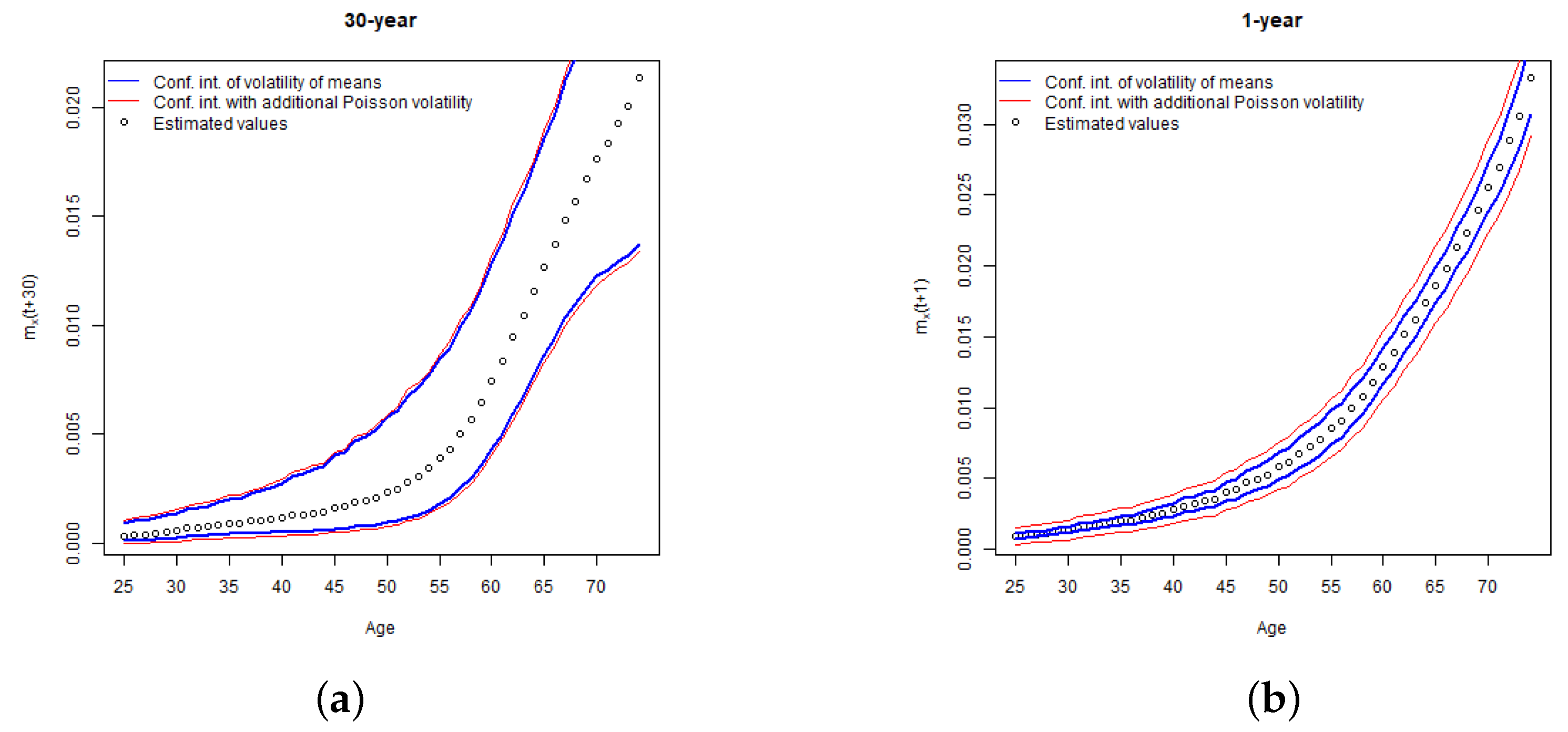
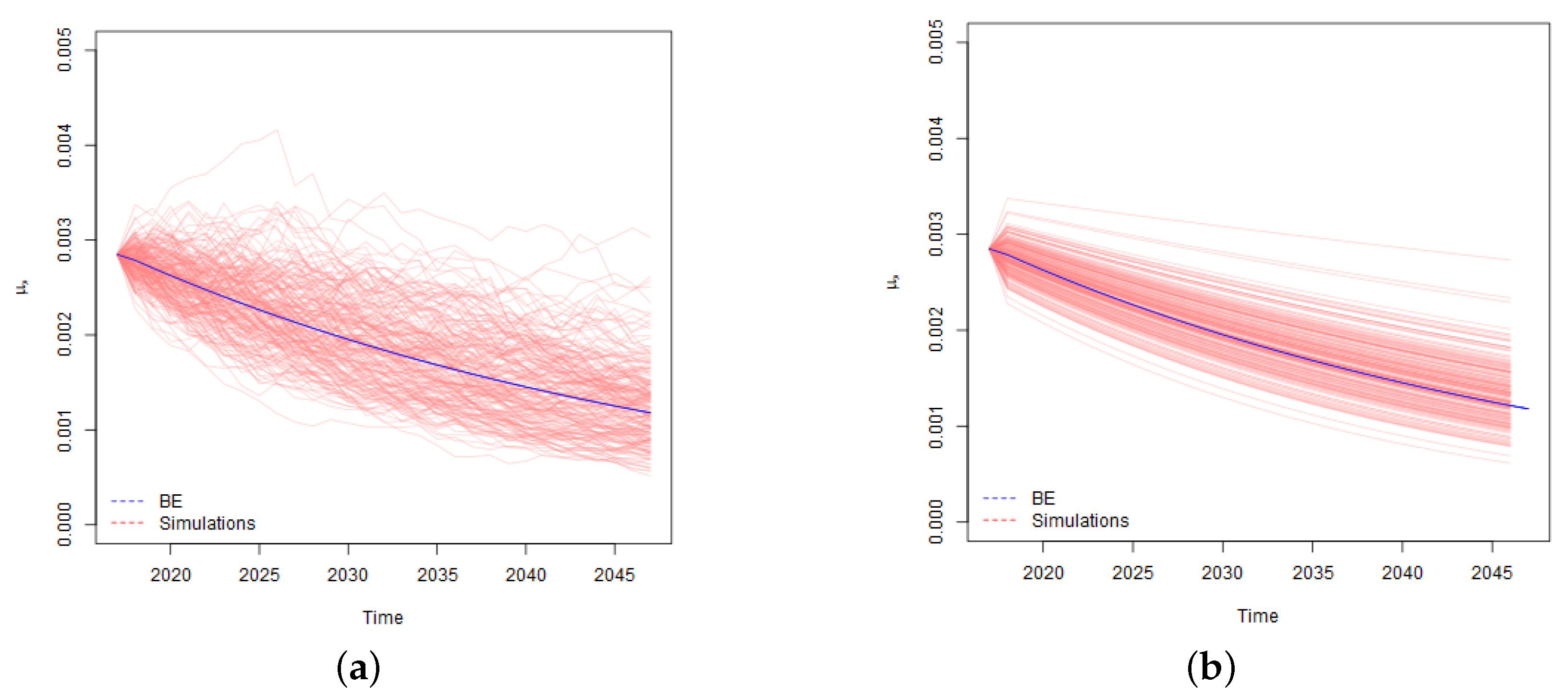
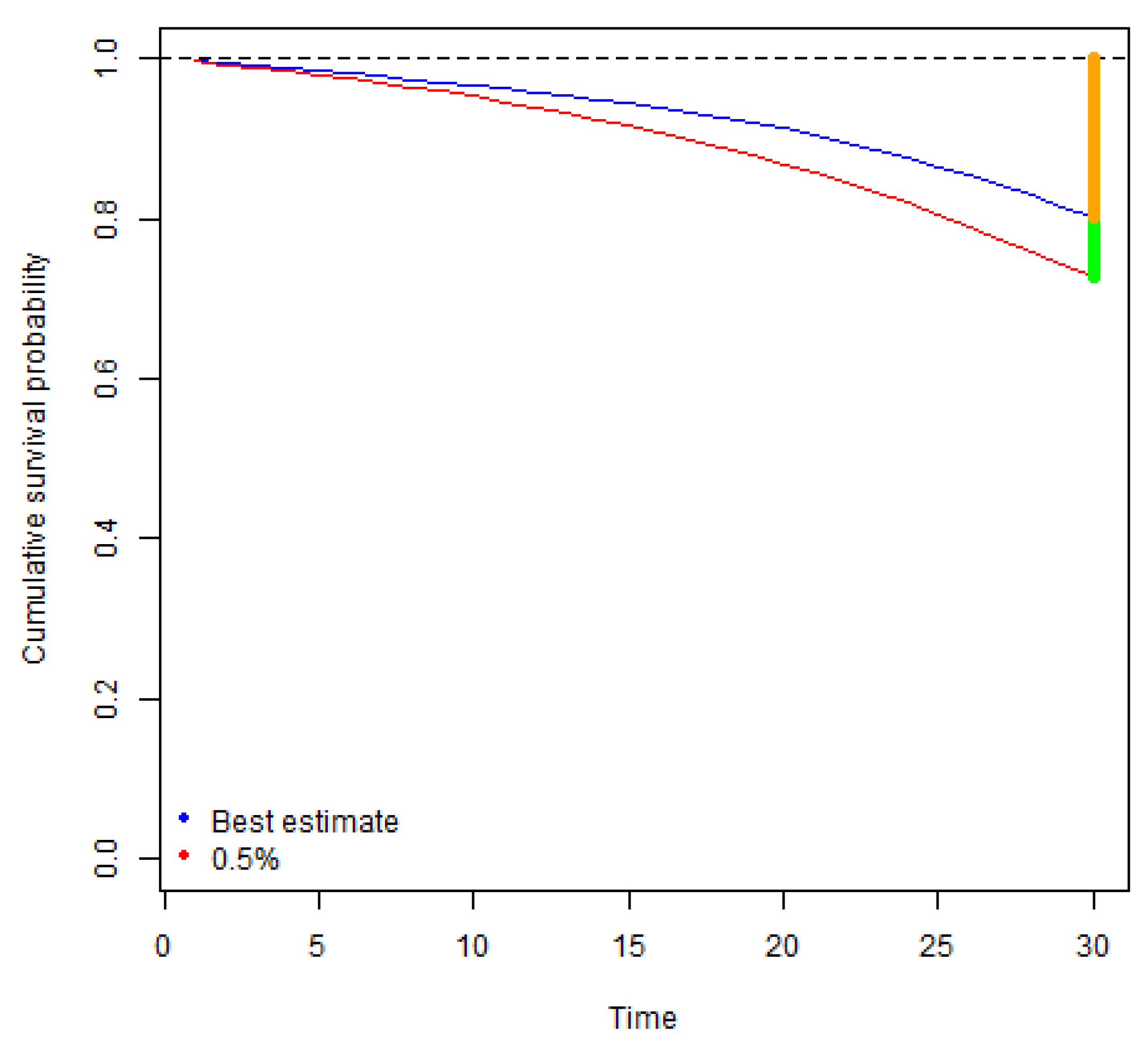
Taking the run-off approach, we consider the fluctuations in mortality rates until the maturity of a policy. In contrast, if we take a one-year view, the key drivers of risk become fluctuation of mortality rates in the first projection year and the risk of changes in reserving (Best Estimate) assumptions at the end of the first projection year. A graphical illustration of the contrast between run-off and one-year simulations of mortality rates is provided in Figure 1.

As illustrated in the charts, in calculation of run-off VaR we apply simulated mortality rates which vary stochastically for the whole period of an insurance coverage. In contrast, in calculation of one-year $\mathrm{VaR}$, we use stochastically simulated mortality rates for modelling of death benefits in the first projection year, and for the remaining years we apply the curves of projected Best Estimate mortality rates, the level and trend of which depend on the outcome of the first year simulations. For example, if a certain simulation scenario stochastically results in a sharp increase of mortality rates in the first projection year, we assume that a curve of the projected Best Estimate mortality rates for that simulation scenario is shifted upwards as well. In addition, the results of the first year simulations, affect the trend of the Best Estimate mortality rates and the projected curves are not parallel. The bigger is the variation in the level and trend, the higher risk is associated with the changes in the Best Estimate technical provisions at the end of the first year, which results in the higher one-year $\mathrm{VaR}$.

Let’s consider what kind of practical reserving behaviour would be consistent with one-year $\mathrm{VaR}$ model described above. Firstly, the model implies that actuaries in the reserving assumptions allow for the future mortality improvements (mortality reduction factors) which are projected with Lee-Carter model. In practice, actuaries often reserve life assurance products without allowing for future mortality improvements, that is, some prudence is left in the Best Estimate, although strictly speaking this is not in line with the legislation. Overstatement of the Best Estimate means that the risk of its insufficiency due to fluctuation in mortality rates and consequently $\mathrm{VaR}$ are lower. Thus, if the Best Estimate for life assurance products is calculated without allowance for future mortality improvements, the company specific one-year $\mathrm{VaR}$ would be lower than one-year $\mathrm{VaR}$ assessed by us.

Secondly, consistently with RWD model applied for modelling of Lee-Carter model time varying index, we assume that variation of the latest year mortality rates is fully translated to shifts in projected Best Estimate mortality curves. This implies, that actuaries base the Best Estimate mortality assumptions on the mortality level implied by the last year’s experience. In practice, actuaries often use various smoothing, averaging and similar methods, as a results of which the variation driven by the mortality level of the last observed year may be taken into account only partially. Application of such techniques may result in lower risk of changes in Best Estimate and lower $\mathrm{VaR}$.

Finally, even if the reserving methodology allows for mortality improvements, the sensitivity of the mortality reduction factors (trend risk) to the last year’s mortality experience may vary from insurer to insurer. In our calculations we use two levels of credibility factor $\delta$ ($5\%$ and $10\%$), which represents variation in reserve risk due to differences in actuarial methodologies applied. The credibility parameter may be interpreted as the proportion of evidence related to the last year’s experience accounted for in setting the assumed mortality reduction factors. Thus, in case of $\delta =10\%$ mortality reduction factors are more sensitive to the last year’s experience than in case of $\delta =5\%$, and the modelled trend risk increases with the growth of $\delta$. See Section 5.2 for more detailed discussion of the trend risk modelling.

Overall, the above considerations imply that our approach results in rather conservative estimate of one-year $\mathrm{VaR}$ for two levels of selected trend risk parameters.

For the purpose of comparability of our results with the Standard Formula mortality stress parameter we have converted the calculated $\mathrm{VaR}$’s to equivalent $\mathrm{VaR}$ rates. We define $\mathrm{VaR}$ rate as g which satisfy the following condition

$$B{E}_t+{\mathrm{VaR}}_{0.005}\left(L\right)=\sum _{i=1}^{n}C{F}_{t+i}^{\left(g\right)}.$$

Here L is random variable of a loss in basic own funds, $B{E}_t$ is the initial Best Estimate, t is the valuation year, n is projection term and $C{F}_{t+i}^{\left(g\right)}$, $i\in \{1,2,\dots ,n\}$, are projected mortality benefits calculated according to the applicable benefit formula by applying the following m year stressed mortality probabilities

$${}_m{q}_x^{\left(g\right)}\left(t\right)=1-\prod _{s=0}^{m-1}\left(1-(1+g){\widehat{q}}_{x+s}(t+s)\right),$$

where x denotes age at time t, ${\widehat{q}}_x\left(t\right)$ are the Best Estimates of one year mortality probabilities and $m\in \{1,2,\dots ,n\}$. In such a way, we search for rate g, which makes the stressed Best Estimate equal to the initial Best Estimate plus $\mathrm{VaR}$. The results of calculation of run-off VaR rates are presented in Figure 2.

The results obtained indicate that run-off $\mathrm{VaR}$ rates tend to increase with policy term. Uncertainty about the future mortality rates grows with time, which leads to wider confidence intervals of mortality rates for long term projections.

Similarly, for the policies with decreasing sum assured, higher sums assured are paid in early policy years when the mortality uncertainty is lower than in later policy years, which implies that run-off $\mathrm{VaR}$ rates are generally lower for policies with decreasing sum assured than for equivalent policies with fixed sum assured.

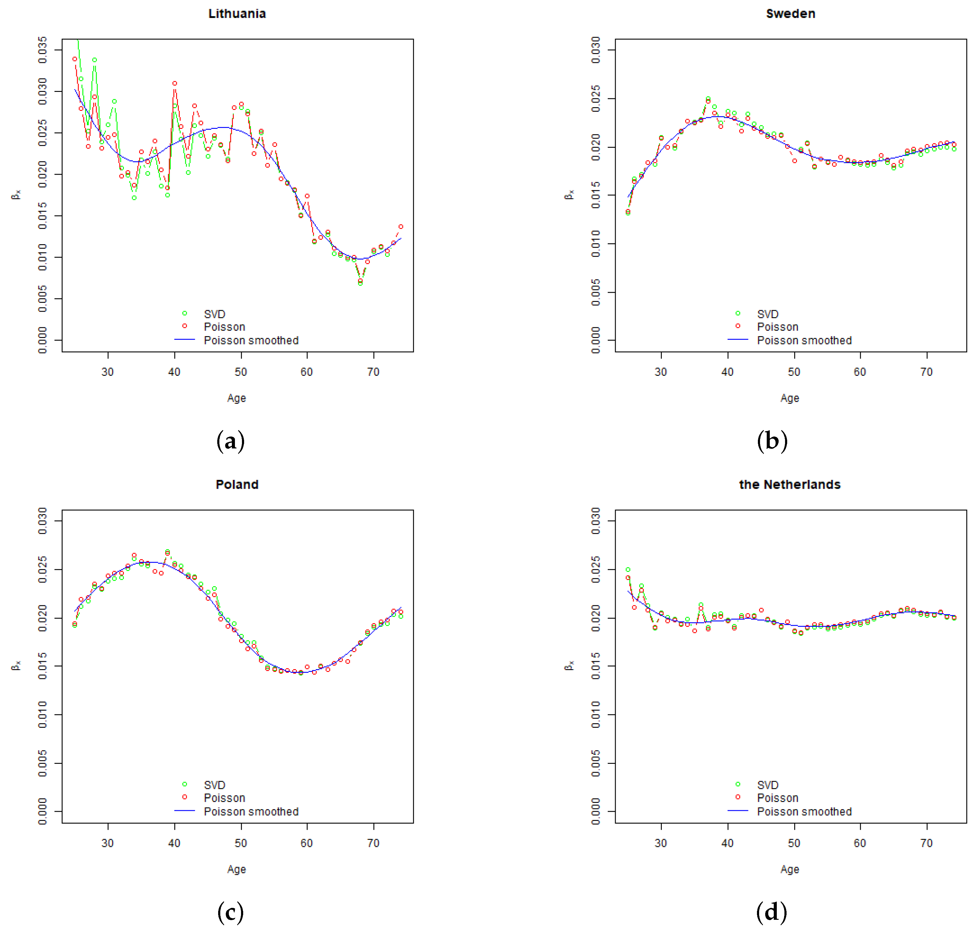
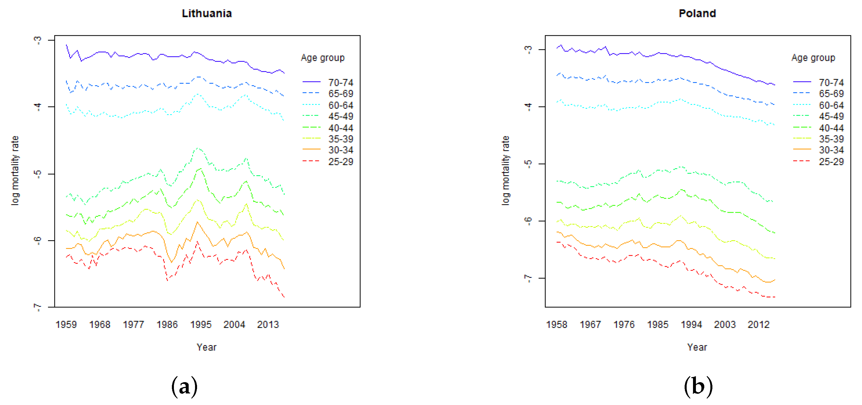
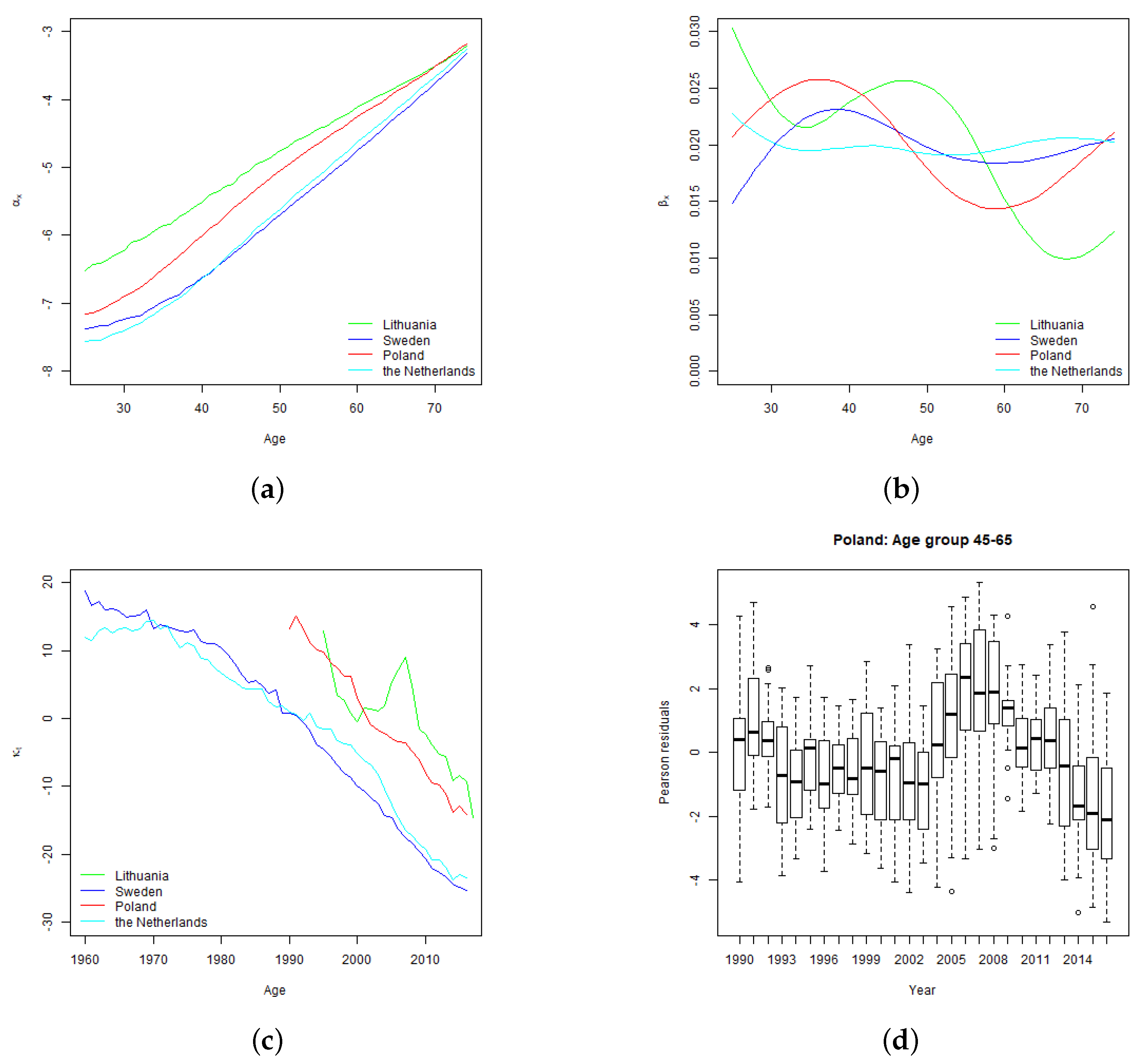
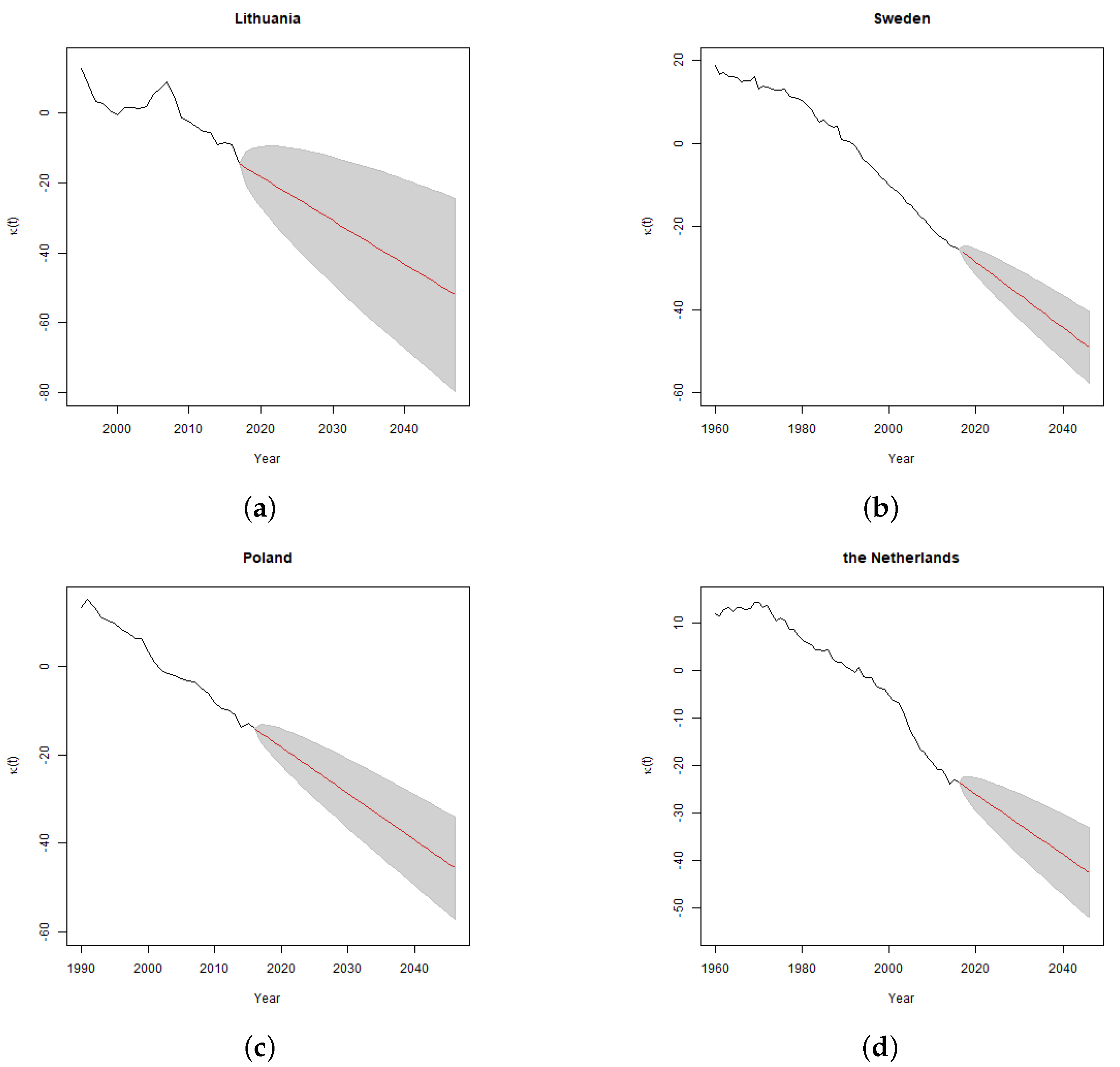
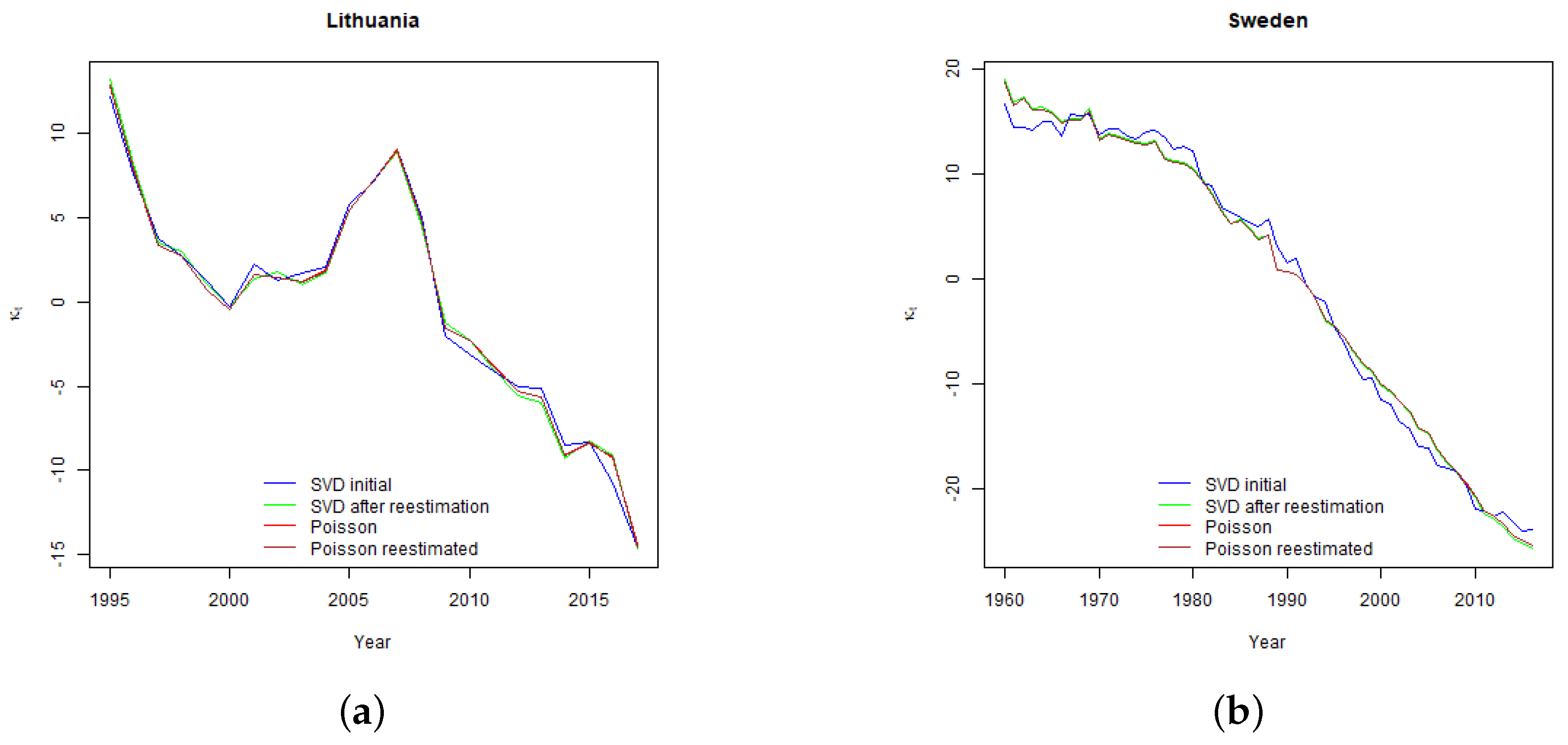
The shape of $\mathrm{VaR}$ rate by age curves is related to the shape of Lee-Carter parameter ${\beta }_x$ (see Section 4) which determines the sensitivity of projected age specific mortality rates to the changes in the time varying parameter, and drives the relative level of age specific projected volatility of mortality rates. As demonstrated in Section 4, Sweden and the Netherlands have relatively stable parameter ${\beta }_x$ over the modelled ages. Consequently, for those countries run-off $\mathrm{VaR}$ rate curves are flat as well. For Lithuania and Poland, higher volatility of mortality rates at younger ages increase the run-off $\mathrm{VaR}$ rates for policies issued to younger policyholders.

Comparing the results with the standard Solvency II stress level of $15\%$, the calculated $\mathrm{VaR}$ rates are significantly higher for Lithuania, however, for other countries the results are close to the value of the standard parameter. As discussed in Section 4, Lithuanian mortality improvement trend is not so settled as in other countries, which resulted in high standard error of time varying index and wide confidence intervals of projected mortality rates.

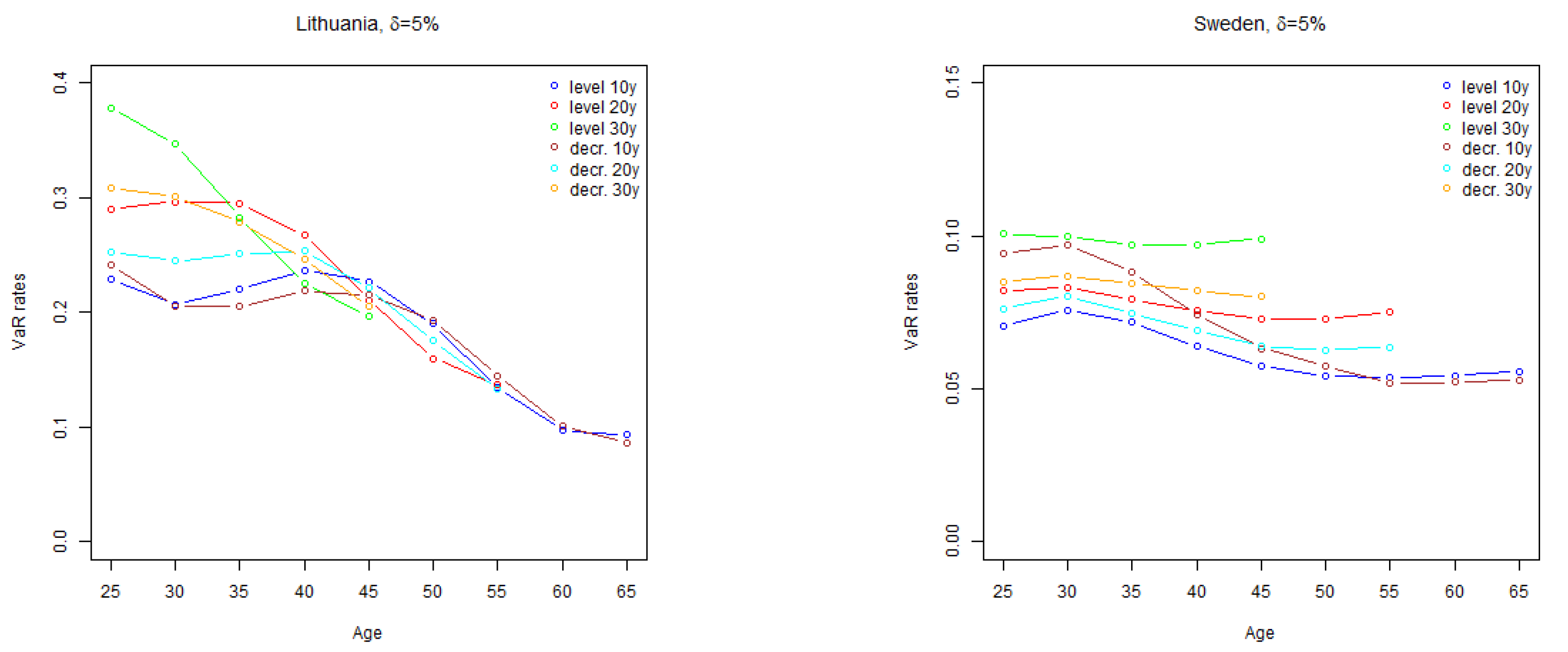
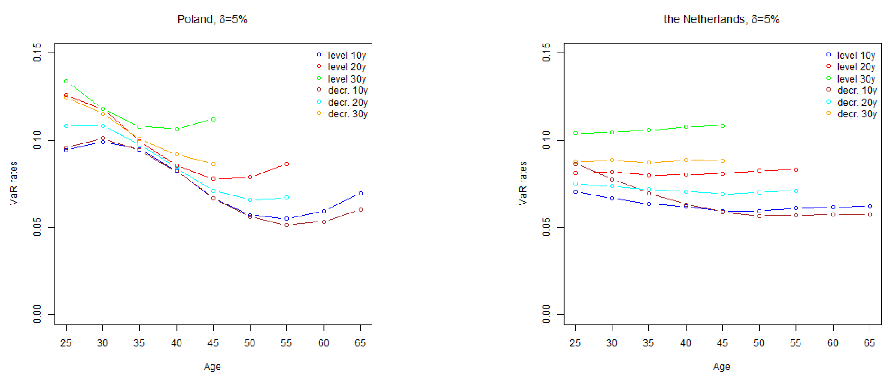
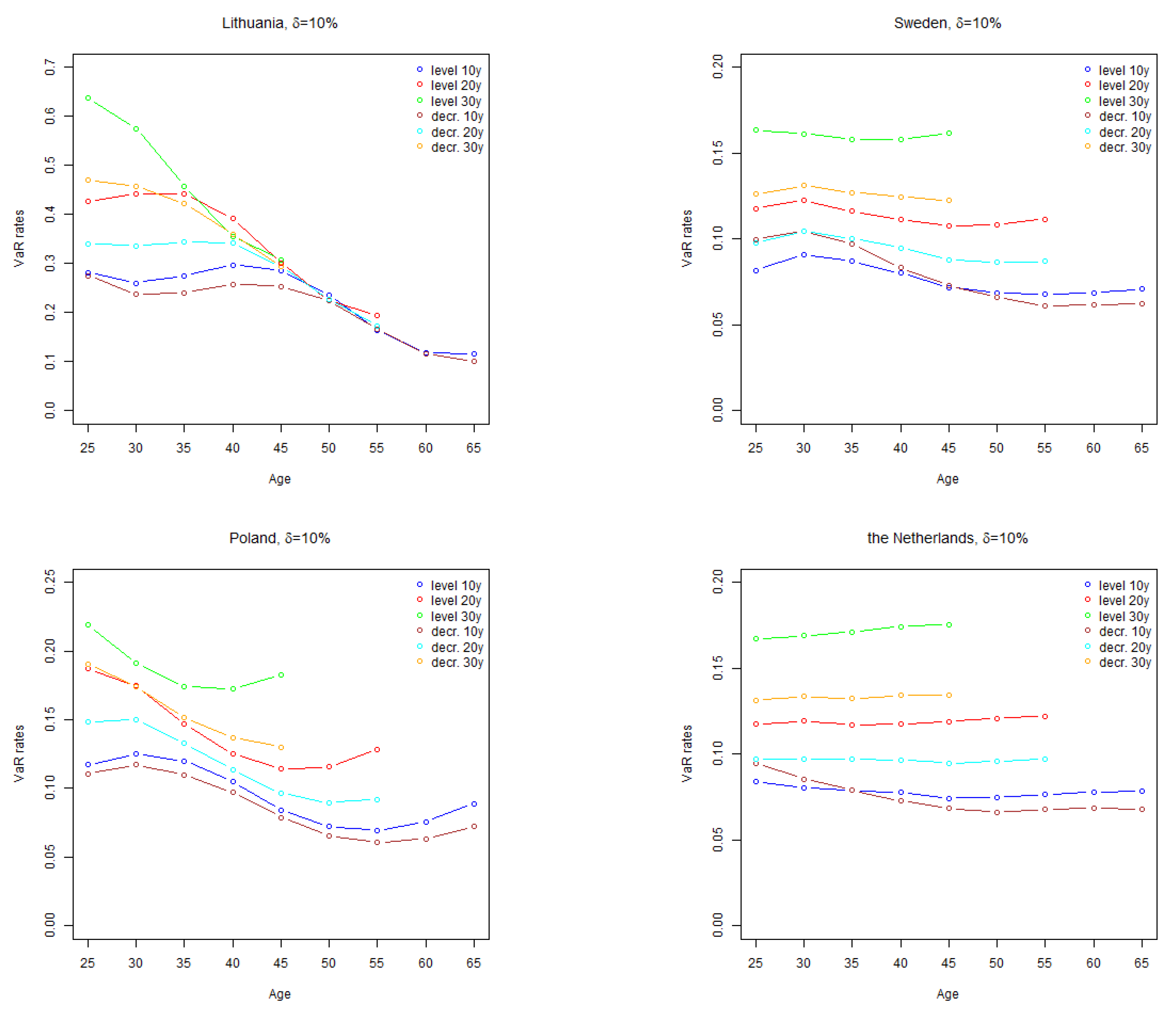
The results of calculation of one-year $\mathrm{VaR}$ for two levels of trend risk parameter $\delta$, are presented in Figure 3 and Figure 4.

The shape of one-year $\mathrm{VaR}$ rate by age curves is similar to the shapes of run-off $\mathrm{VaR}$ rate curves of the corresponding countries. The overall level of the curves to a large extend depends on the value of trend risk parameter $\delta$, especially for longer term policies. For countries other than Lithuania, the overall level of one-year $\mathrm{VaR}$ rates, given the analysed values of parameter $\delta$, tend to be lower than the standard Solvency II mortality stress parameter of $15\%$.

3. Discussion

When comparing the estimated $\mathrm{VaR}$ rates to the Solvency II Standard Formula mortality stress, on average, EIOPA’s calibration looks adequate. Lithuania, which experienced high volatility of mortality of mid-aged population, can be considered as an exception. It is possible, that the mortality trend will stabilize and the width of the confidence bands of the projected mortality rates will become more similar to other EU countries. Meanwhile, actuaries should take into account the risk extra volatility of mortality rates related to Lithuanian exposures.

Overall, the general level of our estimates is comparable with EIOPA (2018). The curved shape of development of EIOPA’s calculated $\mathrm{VaR}$ rates with age is likely to be caused by the shape of Lee-Carter parameter ${\beta }_x$ (see Section 4). Our estimates of parameter ${\beta }_x$ are likely to be different from EIOPA’s due to different range of ages and populations used for model fitting. Nevertheless, actuaries should take into account that mortality $\mathrm{VaR}$ of their insurance portfolios might be higher than the Standard Formula estimate. In particular, in cases of very long term policies with fixed benefits actuaries should consider the need to perform portfolio specific mortality risk assessments.

It should be noted also that some components of mortality risk have been omitted from our assessment. In particular, parameter risk, model risk and basis risk (the risk that the estimates based on the general population data differ from the estimates based on the insured population data) might be significant. In addition, for small portfolios, the risk of random mortality fluctuations might increase the volatility (process risk) substantially. Olivieri and Pitacco (2009) discussed the process risk and showed that it reduces for large portfolios.

In our VaR model we tried not to depart too far from Solvency II interpretation of the mortality risk used by regulators and the market. Consistently with the Solvency II legislation we have not taken into account the risk of catastrophic events (e.g., pandemics) which are allowed for in a separate Standard Formula submodule. By using Lee-Carter model as a basis for the calibration of the stochastic mortality model we have implicitly assumed that the trend observed in the period used for calibration of the model will continue in the future. Considering that the calibration is based on the periods of favorable social, economic and political development, implicitly we assume that there will be no major disturbances (such as wars, long term economic depressions, changes in the political systems, etc.) during our projection period. Modelling of such events would be inevitably subjective and would make our results less comparable with EIOPA (2018).

Basis risk can have a material impact on the results of VaR calculation. Changes in level, trend or volatility of mortality can differ for insured population and the general population, for example, due to differences in the level of income, socio-economic status, regional differences and other factors. However, the effect of the basis risk is difficult to estimate, mainly due to lack of high quality, consistent and sufficient statistical data on mortality of insured lives for an extended time period, which for many countries is not available.

Taking the above into account the results of our calculations should not be interpreted as a comprehensive insurer’s economic capital sufficient to cover mortality risk from all sources of risk with $0.5\%$ probability. Actuaries and risk managers should take this into account when performing realistic mortality risk assessments of their portfolios.

We note that the results of one-year $\mathrm{VaR}$ calculations depend on insurer’s internal reserving procedures and methodologies. It might be the case that the sensitivity of changes of reserving assumptions with experience depends on severity of changes in actual rates: in case of extreme changes in the actual mortality major revision in assumptions is more likely than in case of the minor deviations. Overall, unless there is an established procedure on how the Best Estimate assumptions are updated with the latest experience, the mortality one-year $\mathrm{VaR}$ model and its assumptions will result in substantial simplification in comparison with the real world. However, there are examples of the objective link between experience and Best Estimate assumptions, see Jarner and Møller (2015) for an example of the case where the procedure of updating mortality assumptions is set on the national level. The topic of modelling of the process of updating actuarial assumptions with experience may be an interesting subject for further research. Evidence from such research could help to provide additional justification of one-year $\mathrm{VaR}$ model assumptions and could foster insurers to use such approach more widely in the risk management area.

In addition, analysis of drivers of the mortality improvement and their impact on VaR for mortality risk would be an interesting area for further research. For example, insights from the examination of the effect of changes in smoking habits, obesity, pollution, medical advances and other factors on trend and volatility of mortality could provide valuable input to models and assumptions of VaR for mortality risk. On the other hand, the credibility of such analysis is often compromised by the lack of credible data and complex interdependencies between the mortality data and the underlying drivers of mortality improvement.

In conclusion, based on the analysis performed for the selected countries, we found the overall calibration of the Standard Formula for mortality risk adequate, given the current definition and interpretation of the mortality risk in Solvency II. However, there are insurance portfolio or country specific differences which can result in portfolio specific VaR higher or lower than the capital requirement produced by the Standard Formula.

4. Stochastic Mortality Model

4.1. Overview of the Data

For our analysis we used data from the Human Mortality Database Human Mortality Database (2018) for ages 25 to 74 years. The ages have been selected by considering that the focus of this study is the analysis of mortality (not longevity) risk. In some countries insurers issue whole of life assurance, however, in many countries the largest part of insurers’ exposure to mortality risk is related to mid-ages. The initial overview of the data in Figure 5 shows that development of life expectancy on birth in Central and Eastern Europe (CEE) (Lithuania and Poland) was very different from Sweden and the Netherlands.

Sweden and the Netherlands experienced consistent and almost linear decline in log mortality rates, which correspond to the experience in G7 countries, see Tuljapulkar et al. (2000). The development of mortality rates in Lithuania and Poland was different: improvement of life expectancy in the 1960’s was followed by stagnation in 1970’s and 1980’s. At the beginning of the 1990’s Lithuania, like many other countries of former Soviet Union, experienced a sharp increase in mortality rates. As illustrated in Figure 6, the increase coincided with the collapse of the Soviet Union and the start of the transition to market economy, and was especially high for younger age groups. Several studies investigated this phenomena in different countries of the former Soviet Union. For example, Brainerd and Cutler (2005) investigated six factors which possibly had led to the increase in the Russian mortality and concluded that increase in alcohol consumption and stress caused by the transition are likely to be the key causes of this phenomena. We also note that Poland experienced much lower fluctuation in mortality rates at the beginning of 1990’s than Lithuania.

Since the late 1990’s mortality in Lithuania and Poland started to decline. The growth in the life expectancy in Lithuania was irrupted in late 2000’s when a sharp increase in mortality rates was observed. The increase coincided with the period of global financial and economic crisis which hit Lithuania especially hard. In 2009 at the peak of the crisis the Lithuanian GDP dropped by almost $15\%$ and that was the biggest decline in the EU. In the 2010’s the trend of gradual mortality decline in Lithuania re-established and currently it’s rate is comparable to Sweden and the Netherlands.

4.2. Lee-Carter Model

According to Lee and Carter (1992) mortality rates may be modelled according to the following formula

$$m_x\left(t\right)=exp\{{\alpha }_x+\kappa \left(t\right){\beta }_x+{\epsilon }_x\left(t\right)\},x\in \{1,2,\dots ,A\},t\in \{1,2,\dots ,T\},$$

(2)

where

• $m_x\left(t\right)$ is the central mortality rate for age x in year t,
• ${\alpha }_x$ is parameter, which represents the general shape of changes in log mortality rates with age,
• $\kappa \left(t\right)$ is the time varying index, which represents the general trend of changes in mortality rates with time,
• ${\beta }_x$ is parameter, which determines the impact of the time varying index on age specific log mortality rates,
• ${\epsilon }_x\left(t\right)$ are residuals, it is supposed that ${\epsilon }_x\left(t\right)$ are independent and identically distributed random variables with zero mean and finite variance.

According to the original model fitting procedure, parameters are estimated using two stage procedure. Firstly, $\kappa \left(t\right)$ and ${\beta }_x$ are estimated using singular value decomposition (SVD) of a matrix of log mortality rates minus age specific constant ${\alpha }_x$. Age specific constant may be estimated as an average of log mortality rate for each age group. To ensure that the model is determined, the following two constrains are introduced

$$\sum _{t=1}^T\kappa \left(t\right)=0,\sum _{x=1}^A{\beta }_x=1.$$

(3)

As the second step, after fixing ${\alpha }_x$ and ${\beta }_x$, $\kappa \left(t\right)$ are re-estimated to ensure that the actual historic total number of deaths in a year equals to the fitted number of death.

Brouhns et al. (2002) developed a method of fitting the Lee-Carter model as Poisson regression:

$$D_{\{x,t\}}\sim \mathrm{Poisson}\left(E_{\{x,t\}}{\mu }_x\left(t\right)\right)\mathrm{with}{\mu }_x\left(t\right)=exp\{{\alpha }_x+\kappa \left(t\right){\beta }_x\},$$

(4)

where $D_{\{x,t\}}$ and $E_{\{x,t\}}$ are the number of deaths and the number of exposed to risk respectively, at age x and time t. The motivation for fitting the model with Poisson regression is to avoid the SVD assumption that errors are distributed homoskedastically. The model is overparametrized as the original Lee-Carter model, therefore, the identifiability constrains (3) are used in this model setting as well.

As noted by McCullag and Nelder (1989), in practice, when modelling data with Poisson regression it is not uncommon that the variance of the response variable Y exceeds the variance implied by the model according to which $\mathrm{var}\left(Y\right)=\mathbb{E}\left(Y\right)$. This phenomenon is called overdispersion and may occur due to a number of reasons, one of which is heterogeneity of the modelled population due to features other than factors explicitly taken into account by the model. For example, mortality of same age population may further vary with income level, urban/rural living location, and so forth. Li et al. (2009) allowed for overdispersion in mortality data by expressing Lee-Carter model as Negative Binomial regression. Such approach allows to estimate different overdispersion parameters for each age group. We will take a simpler approach and will estimate only the total overdispersion parameter. The overdispersion parameter will be used for the purpose of assessment of model fit and where appropriate will be taken into account in simulation of random realisations from model (4).

The Lee-Carter model projections are derived using the same basic model structure defined by Formula (2). In the original paper Lee and Carter (1992) assumed that ${\alpha }_x$ and ${\beta }_x$ are fixed and changes in the mortality rates are driven by innovations of time varying index $\kappa \left(t\right)$. In later applications, several methods were developed (see Renshaw and Haberman (2008) and Li (2014) for overview) to take into account uncertainty in other model parameters, however, in majority of applications of Lee-Carter model $\kappa \left(t\right)$ has remained the key source of uncertainty. As a simplification, in this paper we will assume that ${\alpha }_x$ and ${\beta }_x$ parameters are equal to the estimated values and do not change over the projection period.

Under the Poisson regression setting, the two sources of uncertainty are variation of $\kappa \left(t\right)$ parameter, which drives the mean of projected mortality rates, and random variation around the mean, which is also affected by the level of overdispersion. It should be noted, that in the long term projections, random variations around the mean tend to “cancel out” each other, and their effect on long term projections becomes small. However, for one year projections random fluctuations can be significant, see Figure 7 for illustration.

Further in our analysis as a simplification we will not allow for additional volatility random due to variation of mortality rates around the projected mean in run-off $\mathrm{VaR}$ calculation, which is mainly driven by the long term projections of mortality rates. However, we will allow for additional volatility in one-year $\mathrm{VaR}$ calculations, which proportionally is more influenced by the results of the first year projections.

4.3. Estimation of Parameters

Firstly, we considered which time periods should be used for estimation of the parameters. Mortality data for Poland and Lithuania was provided from the end of 1950’s. Due to uneven development of mortality until 1990’s our initial fits of the models for these countries using full data sets were poor. The key reason of the inadequate fit was inconsistent and unstable changes in mortality rates for different age groups. For example, in the early 1990’s Lithuanian mortality of mid age population increased sharply. Meanwhile, mortality of higher age population stayed constant. This trend changed in early 2010’s when the mortality in mid age groups started to decline rapidly.

One possibility to improve the fit is to include in the model the second term of SVD decomposition or additional set of time varying parameters in the Poisson regression. This modification, for example, was applied by Renshaw and Haberman (2003) when modelling the UK data and Booth et al. (2002) in the model fitted to the Australian data. The inclusion of higher order terms improves the fit, however, in most of the cases higher order parameters proved to be less predictable than the main trend of mortality decline with time, which makes the forecasting problematic. For the Lithuanian data similar adjustment was implemented by Ignatavičiūtė et al. (2012) who applied original Lee-Carter model to the Lithuanian data for the time period 1970 to 2005. The adjustment resulted only in marginal improvement of the prediction accuracy of the model and the second order trend parameter was volatile and difficult to predict. Therefore, we will not include higher order terms to improve the fit of our model.

Another simple adjustment to improve the fit as applied by Lee and Miller (2001); Booth et al. (2002) and Tuljapulkar et al. (2000) is to calibrate the Lee-Carter model using only the latest and the most relevant mortality experience. In the Lithuanian case we have refitted the model using the mortality data for 1995–2017. The starting year was chosen by considering that by 1995 all major reforms of transition from Soviet system have already been implemented and by performing the graphical inspection of the mortality trends. In Polish case the fitting period was selected to be 1990–2016 as the reforms of transition to market economy in Poland were implemented earlier and the mortality shock due to transition was lower. For Sweden and the Netherlands the data for 1960–2016 was used.

We have performed the estimation of the model parameters using both the original Lee-Carter model and the Poisson regression approach. When fitting the data with Poisson regression we used the gnm function from $\mathcal{R}$ package gnm. The identifiability constrains (4) were imposed as described by Currie (2016). The estimates of ${\beta }_x$ parameters lacked smoothness (see Figure A1 in Appendix A, and therefore were smoothed with cubic splines with 11 knots and penalty parameter of $0.3$. In order to ensure the internal consistency of parameters, we have refitted the Poisson regression and re-estimated parameter $\kappa \left(t\right)$ using the constraint that ${\alpha }_x$ and ${\beta }_x$ parameters equal to originally estimated ${\alpha }_x$ and smoothed ${\beta }_x$ values. After the refitting we checked that due to smoothing there was no major decrease in the log-likelihood.

Table 2. Proportion of variance explained by the first principal component and estimated overdispersion parameter for fitted Lee-Carter model. Overdispersion was estimated as the sum of squared Pearson residuals divided by the residual degrees of freedom.

Statistics	Lithuania	Sweden	Poland	The Netherlands
SVD estimation: proportion of
variance explained by the first	0.78	0.92	0.96	0.95
principal component
Poisson regression: estimated
overdispersion parameter ${\sigma }^2$	1.63	1.45	3.95	1.34

provides a summary statistics on the fit of the models.

Lithuania has the lowest percentage of variance explained by the first principle component of the SVD. This may be explained by the fact that Lithuania has the highest volatility of parameters ${\beta }_x$ and $\kappa \left(t\right)$, see panels (b) and (c) of Figure 8. Poland has the highest overdispersion parameter, which may also indicate lack of fit. Analysis of the residuals indicates some time dependence of the residuals of mid-aged population with time, see panel (d) of Figure 8. However, for the purpose of our study have accepted the model for Poland on the grounds that overall distribution of the residuals does not indicate major deviations from Poisson model.

Figure 8 summarises the results parameter fitting. Overall, the shape of the general mortality pattern by age (parameter ${\alpha }_x$) is similar for all four countries, although the level of mortality differs, especially for younger ages. The level of the curves for Lithuania and Poland are not fully comparable with the curves for Sweden and Netherlands due to different fitting periods, that is, the Lithuanian and Polish ${\alpha }_x$ provides an indication of average mortality from the early 1990’s and the Swedish and the Netherlands from 1960’s.

The estimated parameter of the general mortality trend with time $\kappa \left(t\right)$ is highly volatile for Lithuania. Sweden and the Netherlands demonstrate consistent and nearly linear decline in the value of the parameter as it can be expected from the results of studies of other developed countries (see, for instance, Tuljapulkar et al. (2000); Renshaw and Haberman (2003); Booth et al. (2002) and Brouhns et al. (2002)). The trend for Poland is also nearly linear, however, it covers much shorter period than Swedish and the Netherlands trends. We note, that overall, the direction of the trend is similar to all four countries. The more detailed information on the estimated parameters is presented in Figure A1 and Figure A2 of Appendix A.

4.4. Modelling of General Mortality Trend Parameter $\kappa \left(t\right)$

After carrying the standard time series model identification procedures, Lee and Carter (1992) proposed to suppose $\kappa \left(t\right)$ to be random walk with drift (RWD):

$$\kappa \left(t\right)=\kappa (t-1)+\mu +\epsilon \left(t\right),t\in \{1,2,\dots ,T\},$$

(5)

where $\mu$ is drift parameter and $\epsilon \left(t\right)$, $t=1,2,\dots ,T,$ are independent and identically normally distributed random errors with zero mean and variance, say ${\sigma }^2$.

$\mathrm{ARIMA}(p,d,q)$ models with parameter d equal to 1, predominantly RWD, were the main model for $\kappa \left(t\right)$ in subsequent applications of the Lee-Carter model using the data of various countries. Therefore, our primary hypothesis is that $\kappa \left(t\right)$ derived from re-fitted Poisson regression can be modelled as a differenced time series with $d=1$. In order to accept or reject this hypothesis we performed statistical testing of unit roots using Philips-Perron and Augmented Dickey-Fuller tests as described by Hamilton (1994) (see Chapter 17).

Philips-Perron test is based on the following regression, in our case, which is fitted using the estimated historical $\kappa \left(t\right)$ values by the ordinary least squares (OLS):

$$\kappa \left(t\right)=\mu +\rho \kappa (t-1)+\delta t+v\left(t\right).$$

In the equation above, $v\left(t\right)$, $t\in \{1,2,\dots ,T\}$ are zero mean residuals, which may be heterogeneously distributed or serially correlated, and $\mu$, $\rho$, $\delta$ are estimated parameters. To test the hypothesis of the presence of unit root the following two statistics are calculated:

$$\begin{array}{ccc}\hfill Z\left(\rho \right)& =& T(\widehat{\rho }-1)-\frac{T^2{\sigma }_{\widehat{\rho }}^2}{2s^2}({\lambda }^2-{\gamma }_0)\hfill \\ \hfill Z\left(t\right)& =& \sqrt{\frac{{\gamma }_0}{{\lambda }^2}}\frac{\widehat{\rho }-1}{{\sigma }_{\widehat{\rho }}}-\frac{T{\sigma }_{\widehat{\rho }}}{2s\lambda }({\lambda }^2-{\gamma }_0),\hfill \end{array}$$

where and in the sequel ${\gamma }_m$ $(m=0,1,\dots ,q)$ is sample auto covariance with m-th lag, q is the maximum lag considered in the test, ${\sigma }_{\widehat{\rho }}$ is OLS standard error of $\widehat{\rho }$, s is the standard error of $v\left(t\right)$, and the quantity ${\lambda }^2$ is calculated using the following formula

$${\lambda }^2={\gamma }_0+2\sum _{j=1}^q\left(1-\frac{j}{q+1}\right){\gamma }_j.$$

The Augmented Dickey-Fuller test is based on the following regression using OLS:

$$\kappa \left(t\right)=\mu +\rho \kappa (t-1)+\delta t+\sum _{i=1}^{p-1}{\zeta }_i\left(\kappa (t-i)-\kappa (t-i+1)\right)+\epsilon \left(t\right),$$

where p is number of lags considered in the test, $\epsilon \left(t\right)$, $t\in \{1,2,\dots ,T\}$, are i.i.d. random residuals with zero mean and finite fourth moments, and $\mu$, $\rho$, $\delta$, ${\zeta }_1,\dots ,{\zeta }_{p-1}$ are the model parameters. To test to hypothesis on the presence of unit root the following two statistics are used:

$$\begin{array}{ccc}\hfill Z_{DF}\left(\rho \right)& =& T(\widehat{\rho }-1)/(1-{\widehat{\zeta }}_1-{\widehat{\zeta }}_2-\dots -{\widehat{\zeta }}_{p-1}),\hfill \\ \hfill Z_{ZD}& =& (\widehat{\rho }-1)/{\sigma }_{\widehat{\rho }}^2,\hfill \end{array}$$

where ${\sigma }_{\widehat{\rho }}^2$ is OLS standard error of $\widehat{\rho }$ and $\widehat{\rho },{\widehat{\zeta }}_1,\dots ,{\widehat{\zeta }}_{p-1}$ denote estimations of corresponding parameters.

Summary of the test results is provided in

Table 3. Statistical testing for unit-roots for the time series parameter of $\kappa \left(t\right)$.

Test Statistics	Lithuania	Sweden	Poland	The Netherlands
Philips-Perron test
$Z\left(\rho \right)$	−6.5 [−17.9]	−2.7 [−19.8]	−19.1 [−17.9]	−4.1 [−19.8]
$Z\left(t\right)$	−1.7 [−3.6]	−1.6 [−3.5]	−3.6 [−3.6]	−2.2 [−3.5]
Augmented Dickey-Fuller test
$Z_{DF}\left(\rho \right)$	−5.8 [−17.9]	−3.5 [−19.8]	−17.8 [−17.9]	−5.4 [−19.8]
$Z_{DF}\left(t\right)$	−1.1 [−3.6]	−2.7 [−3.5]	−2.3 [−3.6]	−1.9 [−3.5]

. The Philips-Perron test statistics were calculated using the pp.test function of $\mathcal{R}$ package tseries. The 2-lags model was used for Lithuania and Poland data and 3-lags model was used for Sweden and the Netherlands data. Critical values at $95\%$ confidence level are provided in the brackets are from Hamilton (1994), (see Tables B5 and B6).

Overall, the results of the tests support the hypotheses that $\kappa \left(t\right)$ can be modelled as time series with unit root. For Poland the first of Philips-Perron tests fails by a small margin, but the results of other tests support the hypothesis of unit root. Thus we select Random Walk with Drift (RWD) as the model for $\kappa \left(t\right)$ for all analyzed countries. We note that in general, depending on the data, other time series models may be more appropriate, as showed Kleinov and Richards (2017) who performed comparative analysis of modelling $\kappa \left(t\right)$ using RWD, ARMA and ARIMA time series models and concluded that for the analyzed UK data on higher age males more complex ARIMA models can better represent time series of time varying parameter than RWD. We also note, that selection of the time series model might have major implications on the width of the confidence intervals of projected $\kappa \left(t\right)$ and, subsequently, calculated $\mathrm{VaR}$. The estimated parameters of time series models (5) for $\kappa \left(t\right)$ are provided in

Table 4. Estimated Random Walk with Drift (RWD) parameters of time series $\kappa \left(t\right)$ derived from the re-fitted Poisson regression.

Parameter	Lithuania	Sweden	Poland	The Netherlands
$\mu$	−1.25	−0.79	−1.05	−0.63
${\sigma }^2$	6.62	0.65	1.14	0.78

.

The drift parameter $\mu$ shows that time varying index is expected to decrease faster in Lithuania and Poland than in Sweden and the Netherlands. Considering that the values of ${\beta }_x$ parameters are comparable for all countries, this implies that mortality in Lithuania and Poland is expected to reduce faster than in the remaining two countries. This may be explained by a higher current level of mortality in CEE countries and the expectations that gradually the level of mortality in CEE countries will become more similar to the rest of the EU. We also note that due to less settled historic mortality experience the estimated variance of time varying index is higher for Lithuania and Poland which leads to wider estimated confidence intervals of the projections, as presented in Figure 9.

5. Methodology of VaR Calculations

5.1. Run-off VaR Methodology

We used the following formula for calculation of run-off VaR:

$${\mathrm{VaR}}_{0.005}\left(\sum _{i=1}^{n}C{F}_{t+i}\right)=inf\left\{l\in \mathbb{R}:\mathbb{P}\left(\sum _{i=1}^{n}C{F}_{t+i}-B{E}_t>l\right)⩽0.995\right\}.$$

(6)

The formula implies that run-off $\mathrm{VaR}$ is simply the quantile of the distribution of the deviation of the sum of total estimated losses till maturity in n years minus the Best Estimate at the end of year t which is calculated as the expected value of future mortality cash flows derived using the central projection of the mortality probabilities

$$B{E}_t=\mathbb{E}\left(\sum _{i=1}^{n}C{F}_{t+i}\right).$$

The distribution of future cash flows is assessed by performing for each projection year ${10}^4$ simulations of random errors $\epsilon$ distributed according Normal law $N(0,{\sigma }^2)$ with standard error estimated in fitting RWD model for $\kappa \left(t\right)$. The simulations are used to derive the simulated paths of the Lee-Carter model parameter $\kappa \left(t\right)$ for time moments $t+1,t+2,\dots ,t+n$. Keeping the parameters ${\alpha }_x$ and ${\beta }_x$ be fixed we derive the simulated mortality probabilities, which are converted to cash flows using the formulas described in Section 5.3.

5.2. One-Year VaR Methodology

In deriving one-year VaR we use the basic Solvency II principle, which requires calibration of SCR to VaR of the (loss of) Basic Own Funds subject to a confidence level of $99.5\%$ over a one-year period. Basic Own Fund ${BOF}_t$ at the end of year t, is defined as the difference between insurer’s assets $A_t$ and liabilities $L_t$, valued according to the Solvency II requirements, plus subordinated liabilities, which we will ignore in our analysis as a simplification. Liabilities $L_t$ may be disaggregated into technical provisions, consisting of Best Estimate $B{E}_t$ and Risk Margin $R{M}_t$, and other liabilities $O{L}_t$. Therefore we suppose that

$$BO{F}_t=A_t-B{E}_t-R{M}_t-O{L}_t$$

for each year t.

In practice, there are many factors which could contribute to the change in the Basic Own Funds over the year. Considering that our focus is on the mortality risk, the analysis was performed for a simplified portfolio of a single premium (payable in advance) fixed term life assurance policies. We assumed that there are no lapses, no expenses, no new business, no changes in other liabilities and that claims are paid immediately after they occur. We also assumed that there are no cash flows to or from a shareholder, such as dividends, capital injections, and that the investment return on assets and the discount rate used for calculation of technical provisions both are zero. Depending in the size of a discount rate, discounting would have a similar effect as a reduction of benefits with time, that is, based on the results presented in Section 2 would generally reduce VaR. Finally, we assumed that Risk Margin is also fixed. In practice, changes in Best Estimate and Risk Margin are likely to be positively dependent and Risk Margin is likely to affect VaR. However, we have accepted this simplification, considering that due to its relative size, Risk Margin is likely to have significantly smaller effect on VaR than the Best Estimate.

Under the above assumptions a change in assets during year $t+1$ is caused only by a cash outflow $C{F}_{t+1}$ due to payment of death claims. Therefore, the random variable of a change in Basic Own Funds during the year $t+1$ can be expressed as follows:

$$\Delta BO{F}_{t+1}=A_{t+1}-A_t-(B{E}_{t+1}-B{E}_t)=B{E}_t-C{F}_{t+1}-B{E}_{t+1}.$$

(7)

Best Estimate for valuation date at the end of the year $t+1$, assessed using the information ${\mathcal{F}}_t$ available at the end of year t is

$$\mathbb{E}\left(B{E}_{t+1}\left|{\mathcal{F}}_t\right)\right)=\sum _{i=2}^n\mathbb{E}\left(C{F}_{t+i}|{\mathcal{F}}_t\right).$$

Inserting this into Equation (7), and assuming that we assess $\Delta BO{F}_{t+1}$ using information available at the end of year t we obtain the following expression

$$\Delta BO{F}_{t+1}=B{E}_t-\left(C{F}_{t+1}+\mathbb{E}\left(B{E}_{t+1}|{\mathcal{F}}_t\right)\right).$$

(8)

Thus, random variable of the change in the Basic Own Funds during the next valuation year is equal to the difference between the initial Best Estimate and the sum random variables of the claims cash flow during the year $t+1$ and the Best Estimate at the end of year $t+1$.

Substituting the result (8) into Formula (1), we get the VaR formula for the loss of the Basic Own Funds over one year (one-year VaR), with the confidence level of $99.5\%$, as assessed using the information available at time t:

$$VA{R}_{0.005}\left(\Delta BO{F}_{t+1}\right)=inf\left\{l\in \mathbb{R}:\mathbb{P}\left(B{E}_t-\left(C{F}_{t+1}+\mathbb{E}\left(B{E}_{t+1}|{\mathcal{F}}_t\right)\right)>l\right)⩽0.995\right\}.$$

(9)

Thus, SCR is the capital required to cover the excess of the total of claims payments during the first projection year and the Best Estimate at the end of the first projection year over the initial Best Estimate with $99.5\%$ probability. We note that random variables $C{F}_{t+1}$ and $\mathbb{E}\left(B{E}_{t+1}|{\mathcal{F}}_t\right)$ are not independent. Actuaries usually reconsider the assumptions used to calculate Best Estimate based on the recent actual mortality experience. For example, significantly higher than expected incurred mortality losses are likely to lead to upwards revision of the Best Estimate mortality assumptions. Therefore, we can presume positive dependence between $C{F}_{t+1}$ and $\mathbb{E}\left(B{E}_{t+1}|{\mathcal{F}}_t\right)$ and our modelling challenge is to estimate conditional expectation

$$\mathbb{E}\left(\sum _{i=2}^{n}C{F}_{t+i}|C{F}_{t+1}\right).$$

There are several ideas how to model this relationship. For example, Richards et al. (2013) for each simulation run added the simulated mortality experience in year $t+1$ to the already available historic data and used the total data set to refit the stochastic mortality model, which enabled to quantify variation in mortality trend parameter. Similarly, Börger et al. (2014) used simulated mortality experience for each stochastic run to re-estimate the mortality trend parameter at $t+1$. We applied a similar approach, and for each run used simulated time varying index $\kappa (t+1)$ of the Lee-Carter model to adjust the RWD drift parameter:

$$\mu (t+1)=\mu +\delta \left(\kappa (t+1)-\kappa \left(t\right)-\mu \right),$$

where $\delta$ is chosen credibility factor and $\mu ,\kappa \left(t\right)$ are parameters estimated during the initial Lee-Carter model fitting (see Section 4.4).

Our approach requires setting explicit credibility factor $\delta$, which is avoided in the methods mentioned above. However, the above methods also rely on certain additional model parameters which control the level of trend risk produced by the simulation. Börger et al. (2014) for the purpose of introducing variability in the slope of the linear trend, re-estimates with weighted least squares the trend using a new stochastic realisation of mortality trend parameter. In this model trend sensitivity is dependent on the choice of the length of the fitting period and the weights used. Similarly, using the approach of Richards et al. (2013), if applied together with Lee-Carter model, trend sensitivity would depend on the selected length of the fitting period. For the purpose of our analysis considering that fitting periods for CEE and non CEE countries differ, we found it more convenient to set an explicit parameter controlling the level of trend risk.

Using the above we firstly take ${10}^4$ simulations of Lee-Carter parameter $\kappa (t+1)$ generated in run-off VaR calculations. They are used to calculate a vector of simulated trend parameters $\mu (t+1)$ which, together with $\kappa (t+1)$ which set the level of forecasted mortality, and are used to derive the curves of forecasted time varying index starting from year $t+2$.

The simulated mortality probabilities are derived as for run-off VaR, except for the allowance for the additional volatility from the mean, as noted in Section 4.2.

5.3. Modelling Different Mortality Benefit Formulas

5.3.1. Level Benefits

Since we assume that there is no discounting, lapses, future premiums and the death benefit does not change during the policy term, we can ignore the timing of death benefits during the period covered by an insurance policy. Therefore, for a policy with sum assured of 1 monetary unit we can calculate the sum of expected cash outflows (death benefits) as the estimated mortality probability over the remaining policy term n:

$$\sum _{i=1}^{n}C{F}_{t+i}={}_n{q}_x\left(t\right),$$

where ${}_n{q}_x\left(t\right)$ is n year death probability assuming that a life aged x is alive at the end of year t, and which can be calculated using the following formulas:

$$\begin{array}{ccc}\hfill {}_n{q}_x\left(t\right)& =& 1-{}_n{p}_x\left(t\right),\hfill \\ \hfill {}_n{p}_x\left(t\right)& =& \prod _{s=0}^{n-1}{p}_{x+s}(t+s)=\prod _{s=0}^{n-1}\left(1-q_{x+s}(t+s)\right).\hfill \end{array}$$

In case of run-off VaR, inserting this into Formula (6) and noting the Best Estimate of term assurance policy with level benefits as $B{E}_t^{\left(L\right)}$, we get that

$$Va{r}_{0.005}^{\left(L\right)}\left(\sum _{i=1}^{n}C{F}_{t+i}\right)=inf\left\{l\in \mathbb{R}:\mathbb{P}\left(B{E}_t^{\left(L\right)}-{}_n{q}_x\left(t\right)>l\right)⩽0.995\right\}.$$

Graphical interpretation of the formula is provided in Figure 10. The Best Estimate of the death payout is equal to the expected death probability over the total policy term (represented by the orange line). Run-off VaR (green line) is the difference between $99.5\%$ quantile of the distribution of the death probability over the total policy term minus the Best Estimate.

In case of one-year VaR, in addition to the first year’s death benefits we calculate the projected benefits starting from year $t+2$, multiplied by the probability of survival in the first year. Inserting to Formula (9), one-year VaR for term life assurance with level benefits can be calculated as follows:

$$VA{R}_{0.005}^{\left(L\right)}\left(\Delta BO{F}_{t+1}\right)=inf\left\{l\in \mathbb{R}:\mathbb{P}\left(B{E}_t^{\left(L\right)}-q_x\left(t\right)-p_x\left(t\right)\mathbb{E}\left({}_{n-1}{q}_{x+1}(t+1)|{\mathcal{F}}_t\right)>l\right)⩽0.995\right\}.$$

5.3.2. Decreasing Benefits

Consider n year term life assurance policy with initial sum assured of 1 which, at the end of each policy year, decreases linearly by $1/n$. Thus, the insurance company is expected to pay 1 if the policyholder has not survived the first policy year, $\left(\right(n-1\left)\right)/n$ if the policyholders died in the second year, and so forth. In such a case, we have

$$\sum _{i=1}^{n}C{F}_{t+i}=\sum _{j=0}^{n-1}\frac{n-j}{n}{q}_{x+j}(t+j){}_j{p}_x\left(t\right)=\frac{1}{n}\sum _{j=0}^{n-1}{}_{j+1}{q}_x\left(t\right),$$

(10)

where the last result is obtained by changing the order of summation and noting that:

$$q_x\left(t\right)+q_{x+1}(t+1)p_x\left(t\right)+q_{x+2}(t+2){}_2{p}_x\left(t\right)+\dots +q_{x+j}(t+j){}_j{p}_x\left(t\right)={}_{j+1}{q}_x\left(t\right).$$

Inserting expression (10) into Formula (6), and noting the Best Estimate of term assurance policy with decreasing benefits by $B{E}_t^{\left(D\right)}$, we get that the run-off VaR for term assurance with decreasing benefits can be calculated as follows:

$$VA{R}_{0.005}^{\left(D\right)}\left(\sum _{i=1}^{n}C{F}_{t+i}\right)=inf\left\{l\in \mathbb{R}:\mathbb{P}\left(B{E}_t^{\left(D\right)}-\frac{1}{n}\sum _{j=0}^{n-1}{}_{j+1}{q}_x\left(t\right)>l\right)⩽0.995\right\}.$$

Graphical interpretation of the formula is provided in Figure 11. The Best Estimate of death payments may be approximated by the orange area times the factor $1/n$. The $99.5\%$ quantile of the distribution of death payments may be represented by the area above the red line times the factor $1/n$, thus VaR is the difference between the two, that is, green area times the factor $1/n$.

We take the same approach to derive the simulated mortality probabilities starting from the year $t+1$ as in the previous subsection. Then the expected benefits starting from year $t+1$ can be calculated using the following formula

$$p_x\left(t\right)\sum _{i=1}^{n}C{F}_{t+i}=p_x\left(t\right)\frac{1}{n}\sum _{j=1}^{n-1}{}_j{q}_{x+1}(t+1)$$

Using equality (10) and the main Formula (9) for one-year VaR for term life assurance with decreasing benefits, we get that

$$VA{R}_{0.005}^{\left(D\right)}\left(\Delta BO{F}_{t+1}\right)=inf\left\{l\in \mathbb{R}:\mathbb{P}\left(B{E}_t^{\left(D\right)}-q_x\left(t\right)-p_x\left(t\right)\frac{1}{n}\mathbb{E}\left(\sum _{j=1}^{n-1}{}_j{q}_{x+1}(t+1)|{\mathcal{F}}_t\right)>l\right)⩽0.995\right\}.$$

References

1. Booth, Heather, John Maindonald, and Len Smith. 2002. Applying Lee-Carter under conditions of variable mortality decline. Population Studies 56: 325–36. [Google Scholar] [CrossRef] [PubMed]
2. Börger, Matthias, Daniel Fleischer, and Nikita Kuksin. 2014. Modeling the mortality trend under modern solvency regimes. ASTIN Bulletin 44: 1–38. [Google Scholar] [CrossRef]
3. Brouhns, Natacha, Michel Denuit, and Jeroen K. Vermunt. 2002. A Poisson log-bilinear regression approach to the construction of projected lifetables. Insurance: Mathematics and Economics 31: 373–93. [Google Scholar] [CrossRef]
4. Brainerd, Elizabbeth, and David M. Cutler. 2005. Autopsy on the empire: Understanding mortality in Russia and the former Soviet Union. The Journal of Economic Perspectives 19: 107–30. [Google Scholar] [CrossRef]
5. Cairns, Andrew J. G., David Blake, Kevin Dowd, Guy D. Coughlan, David Epstein, Alen Ang, and Igor Balevich. 2009. A Quantitative Comparison of stochastic mortality models using data from England and Wales and the United States. North American Actuarial Journal 13: 1–35. [Google Scholar] [CrossRef]
6. Currie, Iain D. 2016. On fitting generalized linear and non-linear models of mortality. Scandinavian Actuarial Journal 2016: 356–83. [Google Scholar] [CrossRef]
7. EIOPA. 2018. EIOPA’s Second Set of Advice to the European Commission on Specific Items in the Solvency II Delegated Regulation. EIOPA-BoS-18/075. Available online: https://eiopa.europa.eu/Publications/Consultations/EIOPA-18-075-EIOPA_Second_set_of_Advice_on_SII_DR_Review.pdf (accessed on 30 October 2018).
8. Hamilton, James D. 1994. Time Series Analysis. Princeton: Princeton University Press. [Google Scholar]
9. Human Mortality Database. 2018. Database Maintained by the University of California, Berkeley, USA, and the Max Planck Institute for Demographic Research, Germany. Available online: https://www.mortality.org (accessed on 15 October 2018).
10. Ignatavičiūtė, Eglė, Rasa Mikalauskaitė-Arminienė, and Jonas Šiaulys. 2012. Lee-Carter mortality forecasting. Lithuanian Journal of Statistics 51: 22–35. [Google Scholar]
11. Jarner, Søren Fiig, and Thomas Møller. 2015. A partial internal model for longevity risk. Scandinavian Actuarial Journal 2015: 352–82. [Google Scholar] [CrossRef]
12. Kleinov, Torsten, and Stephen J. Richards. 2017. Parameter risk in time-series mortality forecasts. Scandinavian Actuarial Journal 2017: 804–28. [Google Scholar] [CrossRef]
13. Lee, Ronald D., and Lawrence R. Carter. 1992. Modeling and forecasting US mortality. Journal of the American Statistical Association 87: 659–71. [Google Scholar]
14. Lee, Ronald D., and Timothy Miller. 2001. Evaluating the performance of the Lee-Carter method for forecasting mortality. Demography 38: 537–49. [Google Scholar] [CrossRef] [PubMed]
15. Li, Jackie. 2014. A quantitative comparison of simulation strategies for mortality projection. Annals of Actuarial Sciences 8: 281–97. [Google Scholar] [CrossRef]
16. Li, Johny Siu-Hang, Mary R. Hardy, and Ken Seng Tan. 2009. Uncertainty in mortality forecasting: An extension to the classical Lee-Carter approach. ASTIN Bulletin 39: 137–64. [Google Scholar] [CrossRef]
17. McCullag, Peter, and John A. Nelder. 1989. Generalized Linear Models, 2nd ed. London: Chapman & Hall. [Google Scholar]
18. Mcneil, Alexander J., Rüdiger Frey, and Paul Embrechts. 2005. Quantitative Risk Management: Concepts, Techniques and Tools. Princeton: Princeton University Press. [Google Scholar]
19. Olivieri, Annamaria, and Ermanno Pitacco. 2009. Stochastic mortality: The impact on target capital. ASTIN Bulletin 39: 541–63. [Google Scholar] [CrossRef]
20. Plat, Richard. 2011. One-year Value-at-Risk for longevity and mortality. Insurance: Mathematics and Economics 49: 462–70. [Google Scholar] [CrossRef]
21. Renshaw, Arthur E., and Steven Haberman. 2003. Lee-Carter mortality forecasting with age-specific enhancement. Insurance: Mathematics and Economics 33: 255–72. [Google Scholar] [CrossRef]
22. Renshaw, Arthur E., and Steven Haberman. 2008. On simulation-based approaches to risk measurement in mortality with specific reference to Poisson Lee-Carter modelling. Insurance: Mathematics and Economics 42: 797–816. [Google Scholar] [CrossRef]
23. Richards, Stephen J., Ian D. Currie, and Gavin P. Ritchie. 2013. A Value-at-Risk framework for longevity trend risk. British Actuarial Journal 19: 116–39. [Google Scholar] [CrossRef]
24. Tuljapulkar, Shripad, Nan Li, and Carl Boe. 2000. A universal pattern of mortality decline in the G7 countries. Nature 405: 789–92. [Google Scholar] [CrossRef] [PubMed]
Figure 1. Example of simulations of central mortality rates (for a fixed age) used for the purpose of calculation of run-off VaR (see (a)) and one-year VaR (see (b)). The calculations are based on the Lithuanian data for a life aged 40 years. In calculations of one-year VaR reserve sensitivity parameter δ = 10% was used.
Risks 07 00058 g001
Figure 2. Calculated run-off VaR rates at policy inception by country for different ages at policy inception, three different terms to maturity (10 years, 20 years and 30 years) and two benefit formulas (level sum assured and sum assured decreasing with time).
Risks 07 00058 g002
Figure 3. Calculated one-year VaR rates (parameter δ = 5 % ) at policy inception by country for different ages at policy inception, three different terms to maturity (10 years, 20 years and 30 years) and two benefit formulas (level sum assured and sum assured decreasing with time).
Risks 07 00058 g003aRisks 07 00058 g003b
Figure 4. Calculated one-year VaR rates (parameter δ = 10 % ) at policy inception by country for different ages at policy inception, three different terms to maturity (10 years, 20 years and 30 years) and two benefit formulas (level sum assured and sum assured decreasing with time).
Risks 07 00058 g004
Figure 5. Development of periodic life expectancy at birth in Lithuania (a), Sweden (b), Poland (c) and the Netherlands (d) according to data from Human Mortality Database (2018).
Risks 07 00058 g005aRisks 07 00058 g005b
Figure 6. Development of log mortality rates in Lithuania (a) and Poland (b) according to data from the Human Mortality Database (2018).
Risks 07 00058 g006
Figure 7. Confidence intervals for 30-year projection (a) and 1-year projection (b) of mortality rates with and without taking into account the additional volatility from random fluctuation around the modelled mean mortality rates. The calculations were performed for Lithuanian data by assuming Gaussian approximation of Poisson distribution and by allowing for overdisperion.
Risks 07 00058 g007
Figure 8. Lee-Carter model parameters α x (panel (a)), β x (panel (b)) and κ ( t ) (panel (c)) estimated using Poisson regression (with re-fitting). Panel (d) shows distribution of Pearson residuals for ages 45–65 in Poland.
Risks 07 00058 g008
Figure 9. Fitted and forecasted κ ( t ) parameters modelled as RWD using data of Lithuania (a), Sweden (b), Poland (c) and the Netherlands (d). The shaded error represents 95 % confidence interval of the projections assuming normal distribution of errors.
Risks 07 00058 g009
Figure 10. Calculation of the Best Estimate (orange line) and run-off VaR (green line) for term life assurance with level sum insured for the policy term of 30 years. The red line represents 0.5 % confidence interval of the survival probability, which is equivalent to 99.5 % confidence interval of the cumulative death probability.
Risks 07 00058 g010
Figure 11. Calculation of Best Estimate (orange area) and run-off VaR (green area) for term life assurance with linearly decreasing sum insured for the policy term of 30 years. The red line represents 0.5 % confidence interval of survival probability, which is equivalent to 99.5 % confidence interval of the cumulative death probability.
Risks 07 00058 g011