1. Introduction
Banks’ loan operations issue long-term loans at relatively high fixed interest rates and fund these loans with their own equity, low interest customer deposits, and short-term loans borrowed from the open market. However, since the short-term loan rate fluctuates with the health of the economy, bank loan operations always involve risk. Since the 2008 financial crisis, many researchers have pointed out that banks’ over leveraging on their loan balance sheet was one of the main triggers of the crisis. On the other hand, the interest rates difference between a long-term loan and a short-term loan normally is in the range of 2–3 percent annually. If a bank is too conservative on short-term borrowing, it will lose profit opportunities. Thus, establishing the right leverage level becomes an important issue.
Limiting the leverage will hold down credit access and disrupt economic growth since it is a built-in process of the banking business.
Gornall and Strebulaev (
2013) built a quantitative model of banking that explains bank capital structure and the decisions of banks and their borrowers. Their analysis gives great knowledge on fundamental questions about the behavior of nature.
Harding et al. (
2013) studied the effect of capital requirements, deposit insurance, and franchise value on a bank’s capital structure. They found that banks that are regulated accordingly preferred to maintain capital above the minimum required. The deep and accurate understanding of the model gives guidance to the discussion of financial regulatory reforms.
The recent financial crisis in 2008 also emphasized the importance of appropriate risk management. Banking experts and researchers have been highly engaged to find methods to manage risks effectively and efficiently in the balance sheet while maintaining profitability.
Birge and Judice (
2012) proposed a balance sheet management problem which contains the main risks. It is an optimization problem to determine a bank asset-liability management strategy by a simulation of bank balance sheets, using time series analysis, over time for multi-period model, and optimizing the utility function of equity for the single-period model.
Retail deposits are considered the core liabilities of the banking sector and the other components of bank funding as the non-core liabilities as in
Hahm et al. (
2013). The rate of credit growth relative to the trend of the risk premium is reflected by the ratio of the non-core to core liabilities. This gives an overview of the risk premiums as one of the main functions in the economy.
Hahm et al. (
2013) formulate a model of credit supply as the reverse of a credit risk model where a large stock of non-core liabilities serves as an indicator of the erosion of risk premiums. Therefore, they are exposed to the possibility of an economic crisis. They found supporting empirical evidence in their study of emerging and developing economies.
The model used in this research extends that of
Birge and Judice (
2012) by viewing the problem as a portfolio optimization problem with one risky asset. The growth optimal portfolio (GOP) theory of
Kelly (
1956),
Thorp (
1971,
2011) and
MacLean et al. (
2011) and its extension by
Vince and Zhu (
2015) has been applied to the model that is discussed in detail in the model chapter. We calibrated historical information of interest rates and defined a random variable
X as the net rate difference of higher long-term loan interest and the lower short-term wholesale interest. GOP theory uses the function:
This is simply the log expected return under the log utility function, which is concave and has a unique maximum in the case of one risky investment. This maximum is often referred to as the Kelly optimal allocation size .
The results of calibrating the historical US loan interest rates shows that the leverage level of the US major banks right before the 2008 financial crisis was 20–30 times of bank equity. This level was close to what is suggested by the growth optimal portfolio theory in
Latane (
1959), a well-known theoretical optimal leverage. On the other hand, it is well known that the growth optimal portfolio theory does not adequately account for investment risk. Kelly’s point may be a large fraction when the wager is favorable and the risk of loss is very small. For such a large fraction, if the loss has occurred, then the amount left may be a small fraction of what one had initially; it may be even less than the initial size if the loss has occurred in more than one consecutive period. An example can be found in
Ziemba and Hash (
1986).
MacLean et al. (
2010), discussed these properties of the Kelly criterion and the idea of “fractional Kelly”. To overcome this risk, an alternative approach was recently developed by
Vince and Zhu (
2015), which modifies the growth optimal portfolio theory to more explicitly account for the risk. Besides the leverage level suggested by the growth optimal portfolio theory, their analysis also suggests two other reasonable risk-adjusted optimal leverage levels: The return to drawdown ratio optimal and the inflection point of marginal increase of return. Using the historical interest data in the US, the alternative two optimal points yield optimal leverage levels that are around 5–8 times that of bank equity. These leverage levels are much more conservative than the Kelly point.
The approaches suggested by Vince and Zhu essentially account for the expected drawdown risk approximated by the position size and are much easier to implement in practice than the alternatives, such as utility maximization, which needs a risk aversion coefficient which is difficult to calibrate. Drawdown is probably the most relevant risk measure in practice since while most risk measures usually focus on an outcome over a one-period horizon, such as value at risk or expected shortfall, in the case of banks it is important to account for periods of consecutive losses, as it is the case of drawdown. It is known among both theoretical researchers and practitioners that the drawdown accounts for portfolio losses better in the long run. Moreover, limiting drawdowns helps smooth the performance of investments. Finally, in real investment drawdown is where investors feel the pain investors. We refer to
Chekhlov et al. (
2005);
Grossman and Zhou (
1993) and
Maier-Paape and Zhu (
2018) and the references therein for additional discussion on drawdown. From the point of view of risk allocation, the inflection point is also highly relevant. It is the point at which the marginal change of return with respect to the risk turns from an increase to a decrease. Thus, it represents the risk level at which it would be more efficient to allocate capital to other projects or other corporations. The risk that is not incurred by using the inflection point can therefore be used in other projects or corporations where the marginal increase in profitability is higher per unit of risk.
Next, we turn to the more challenging issue of sensitivity analysis—how does the change in parameters impact the optimal leverage level? The focus is on the impact of change of short term interest rates on the optimal leverage level. Then analysis has been done on how to use the changes of a loan portfolio to mitigate the need to change the leverage level. Both are pertinent issues in practice. A sound quantitative analysis provides a theoretical foundation for important bank business decisions. However, these issues are mathematically challenging. The foundation for the sensitivity analysis is to calculate the derivatives of the optimal leverage levels with respect to the changes of return and loan portfolio mix. The available data is limited but can be used to estimate the general leverage level. Unfortunately, they are clearly insufficient to estimate the derivative numerically. Empirically, the PERT distribution fits the data series best by using the maximum likelihood method. This provides a handle on the problem. However, analyzing the qualitative behavior of the derivatives is still non-trivial. Formulae have been developed for the derivative of the growth optimal leverage level with respect to the expected return and show that this derivative is positive. In other words, qualitatively, if the environment becomes more profitable for loan operations, then it is reasonable to increase the leverage level. This confirmed the intuition of practitioners’ experiences. The formula for the derivative also enables us to estimate quantitatively the adjustment needed for the leverage level as the economic environment changes. However, a similar qualitative analysis for the return to drawdown ratio optimal and the inflection point turns out to be much more involved and has eluded us so far. Therefore, we approximated using the Taylor expansion and numerical analysis. This derivation guaranteed high accurate approximations that informs practitioners about the correct amount of changes of either the leverage level or the loan portfolio changes to respond to different loan profitability scenarios. Once the optimal points were in hand, the performance was tested using US historical data and comparing different strategies. Firstly, a test was developed for the three optimal leverage levels to investigate which one performs better in terms of risk adjusted return. As the theory suggested, Kelly’s point should give the highest return, which has very high risk, then the return–drawdown ratio and the inflection point respectively, which lower the risk and provide better risk-adjusted returns. Secondly, we performed a test, with the most conservative leverage level (inflection point), to compare changing the optimal leverage level with (Fed) interest rates changes vs. fixing the leverage level.
The final step provides practical strategies for a bank loan operation during different phases of the monetary policies of increasing or decreasing short-term interest rates. Possible adjustments of the loan portfolios include: (1) Adjustment of the leverage level or (2) adjustment of the allocation of 15-year and 30-year loans. This leads to the derivatives’ development of three allocation levels with respect to the return and the allocation percentages. Then we simulated the historical data to compare the above two strategies of adjusting the allocation between 15-year and 30-year loans to fixing the leverage level according to the aggregated data. This analysis provides a reasonable leverage level for banks’ mortgage operations. Moreover, adjustment strategies are suggested for the loan operation in order to deal with different monetary policy environments.
3. Estimating the Leverage Level
This chapter estimates the appropriate leverage levels for the bank loan balance-sheet according to the methods discussed in chapter 03 using, historical data from the US market. Furthermore, this section discusses the data sources and simulation results for two different maturities of loans in the US using the leverage level discussed in chapter 02. Then we compare the existing results with our calculation results. The simulation shows and points are appropriate levels to consider in practice and point is too risky. Finally, we discuss the importance of sensitivity analysis.
3.1. Description of Data
The following data was obtained from the Federal Reserve Bank of St. Louis for:
A 5-year treasury constant maturity rate, percent, annual, not seasonally adjusted (1954–2016).
A 30-year fixed rate mortgage average in the United States, percent, annual, not seasonally adjusted (1971–2016).
A 15-year fixed rate mortgage average in the United States, percent, annual, not seasonally adjusted (1992–2016).
The above data have different lengths. Therefore we must fill the missing values by extrapolating the available data. The following method of calculation was used.
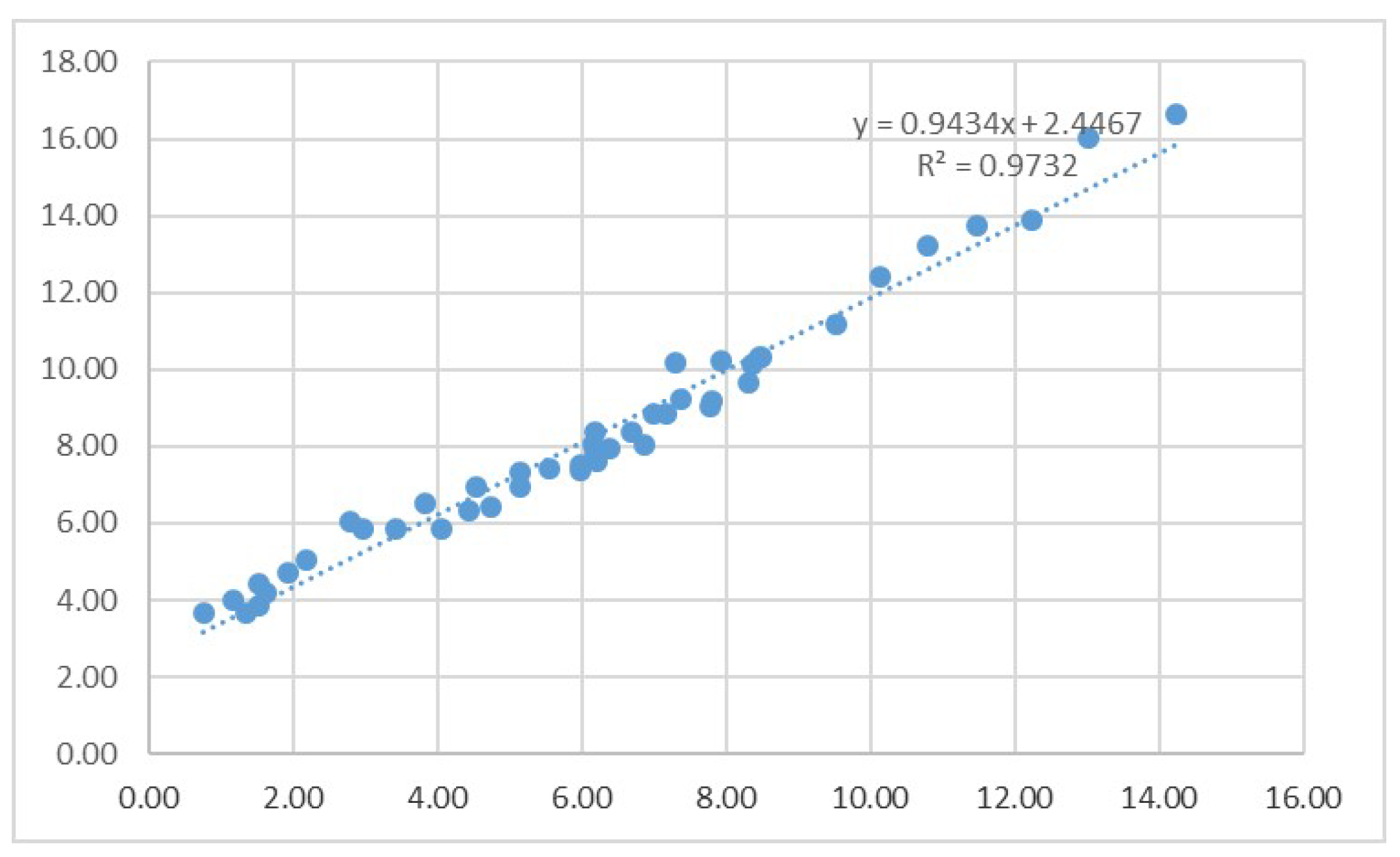
3.1.1. Projecting 30-Year Maturity Interest Rates from 1954 to 1970
Historically, the difference between the long-term mortgage rates and the short-term 5-year treasury rates has been relatively stable. Thus, we use the available data of 30-year maturity interest rates (
Appendix C) and 5-year treasury rates(
Appendix C) from 1971–2016, and fit a linear regression to predict the missing values of the 30-year mortgage rates from 1954–1970 (
Figure 1).
The regression equation is:
which is used to complete the values of 30-year mortgage rates from 1954–1970, since we have 5-year treasury rates from 1954–1970. See
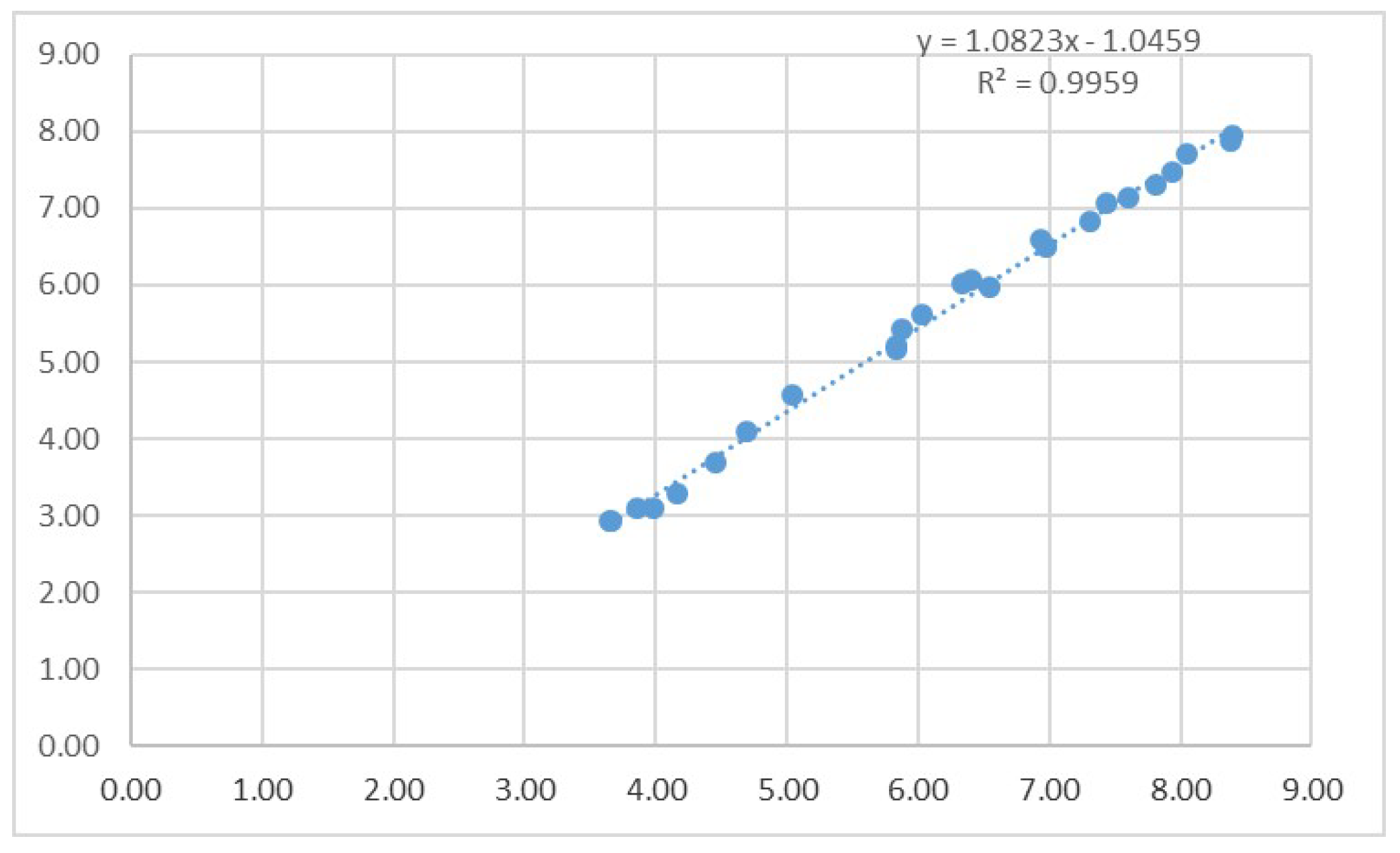
3.1.2. Projecting 15-Year Maturity Interest Rates from 1954 to 1991
The rate difference between the 30-year and the 15-year mortgage is more stable than the difference between the 30-year loan and the short term borrowing rate. Thus, we use the available data of the 15-year maturity interest rates and 30-year mortgage rates from 1992–2016, and fit a linear regression to predict missing values of the 15-year mortgage rates from 1954–1991 (
Figure 2).
The regression equation is:
which is used to complete the values of the 15-year mortgage rates from 1954–1991, since we have 30-year mortgage rates from 1954–1991 from the prediction above.
3.2. Numerical Simulation
We use historical data from 1956–2016 on US yearly loan rates as discussed in the previous section. This data includes two loan rates for two maturities: 15-year and 30-years of loans. It also includes a wholesale rate, which is the rate the bank borrows in the short term to fund the loans (
). In the previous chapter, we calculated formulae for
, and
in Equation (
11) for the net rate. Using those formulae and computer programing (
R), we calculate net rates
X and
Y. Then we find the three critical leverage levels.
Computation Results
In this section, we present our numerical results of three optimal leverage levels using the historical data described above. The calculations are based on
,
(
A1), and the operating cost
for different maturities of loans.
Table 1 and
Table 2 show the optimal leverage levels for different investment horizons
, and 20. The investment horizon,
Q, represents how long the bank is expected to follow this strategy. The decision has to be taken by bank managers.
The relationship among those three optimal points is clear as follows:
where
is the inflection point,
is maximum of the return–drawdown ratio, and
is Kelly’s optimal point.
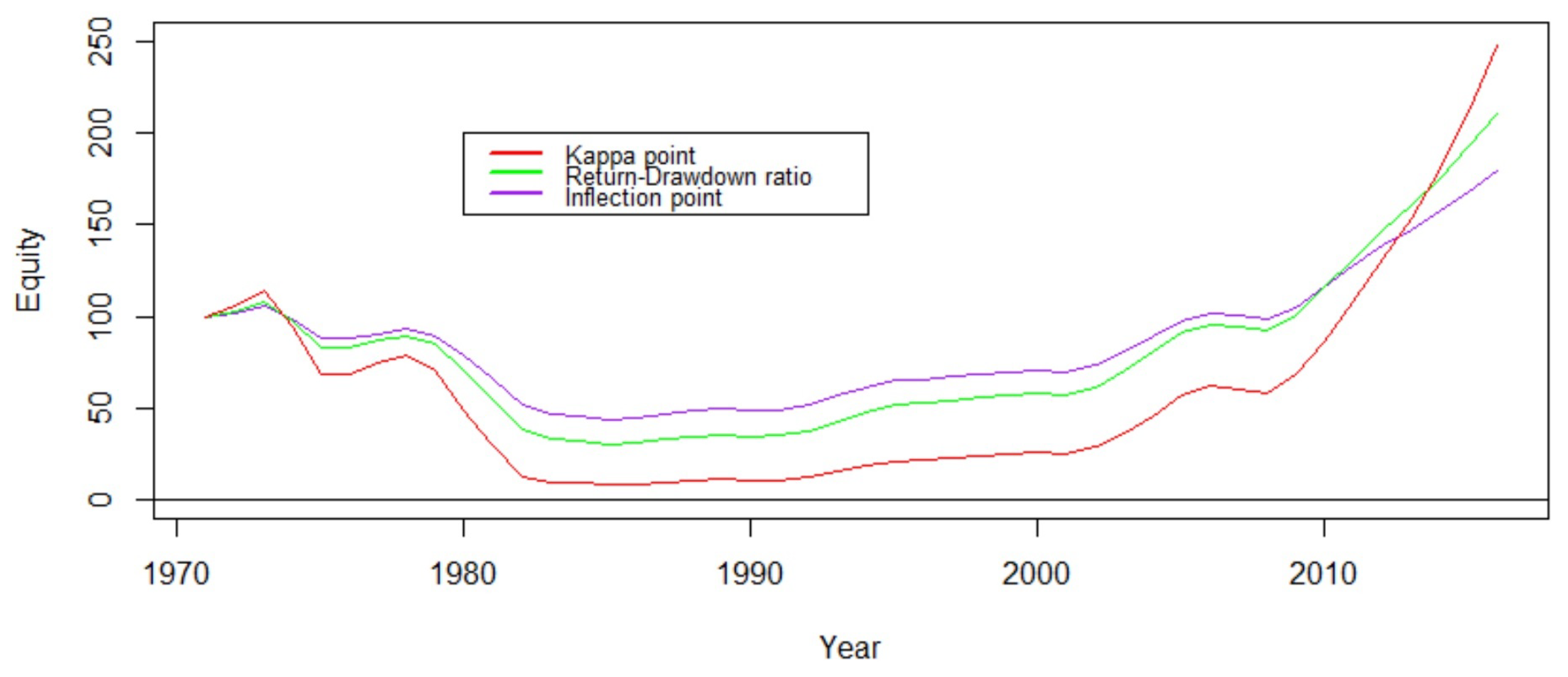
Kelly’s optimal point yields a larger return, but it is too risky for investments shown by simulation in the data (
Figure 3). Return–drawdown ratio maximizes your return adjusted to the investment size as a proxy for risk. If you go beyond
you could gain more but the percentage of the gain will be lower. The inflection point is the lowest. Before the inflection point your rate of return is increasing (derivative is positive or convex) and afterward, it will be decreasing (derivative is negative or concave).
3.3. Performance Comparison
To see the effect of the three leverage levels , , and , we conduct a simulation of the following analysis for the 30-year loan for 50-years investment horizon. All three points are calculated using all historical data. Assuming E (equity) starts with 100 in 1970, then deposits are and respectively. We process this for all years from 1971 through 2016 and plot the return from each three points vs. year (in x-axis). The comparison uses two accounting methods to compare the performances assuming:
Varying equity and;
Fixed equity.
It turns out that the point performed better in the sense that it has a lower risk than the other two in an increasing pace of Fed interest rates in both methods.
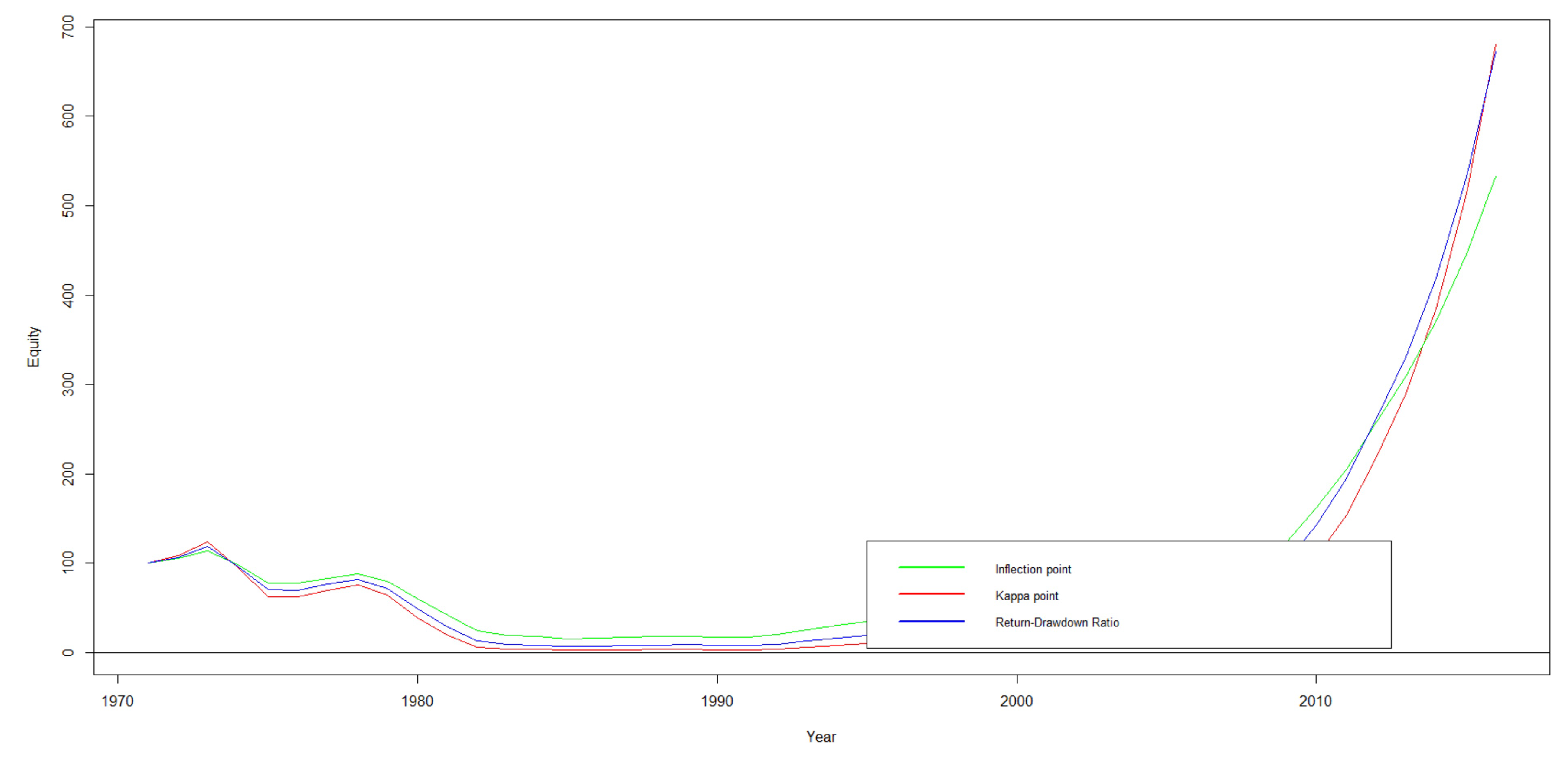
3.3.1. Varying Equity
The varying equity method accumulates the return from the previous year. If there is a profit, then the equity increases, else it decreases. This assumes bank does not distribute profits as dividends to their shareholders or issue any new shares.
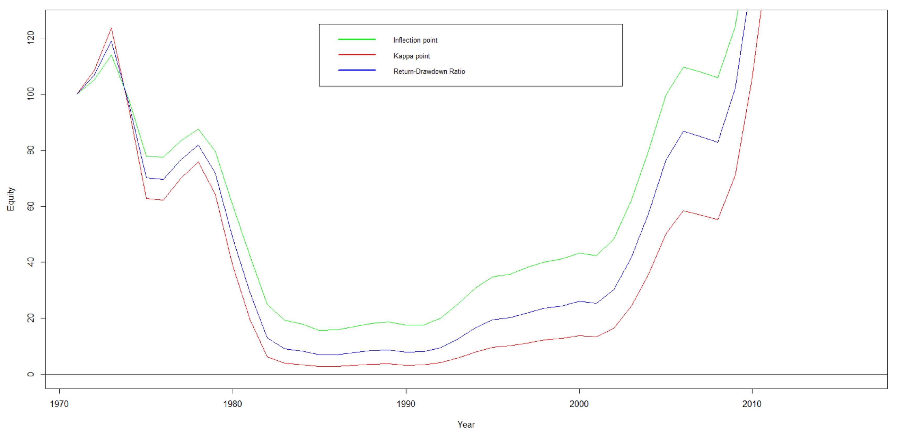
The performance test for the varying equity method shows that the bank almost reaches bankruptcy when using
point, and that the inflection point
performs better in the sense that it has a lower risk compared to the Kelly’s investment size and return–drawdown ratio. Therefore,
point is the safest. The following graph (
Figure 3) shows how equity changes and also shows that around 1981, equity reduced to almost zero when using
point.
Figure 4 provides a better view.
3.3.2. Fixed Equity
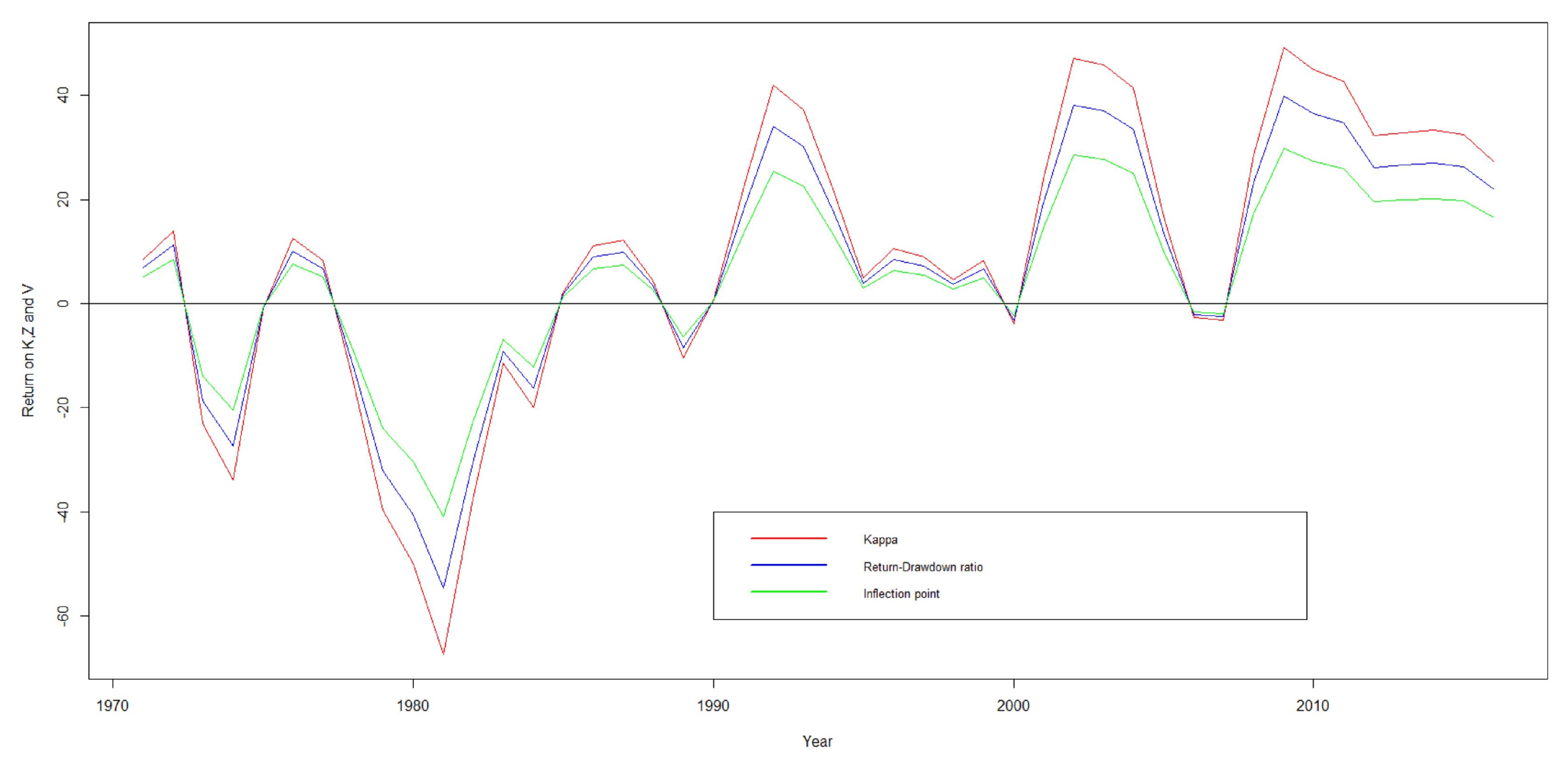
Graph (
Figure 5) shows how individual points perform (year (
X) vs. return (
Y)) when fixing equity. Negative returns occur in the period of interest rates increase by the Federal Reserve Bank.
It shows that has the highest loss and highest profit where risk is higher and it is the maximum of Kelly’s cumulative return curve. The lowest loss is shown by the point and this confirms that the inflection point is more conservative than the other two. It performs better in the sense of generating a risk-adjusted return.
In the next chapter we discuss sensitivity analysis, how the leverage amount can be changed when the Fed interest rates change, or simply how to switch the allocation between loans of different maturities. Then we compare the performance of these two strategies at the end of the next chapter.
3.4. Comparison with Existing Results
In recent years, many other researchers have also studied the bank loan leverage levels using different approaches.
Harding et al. (
2013) studied the impact of capital requirements, deposit insurance, and franchise value on a bank’s capital structure assuming that the market value follows a standard geometric Brownian motion process. The maximum leverage reported is
and the minimum leverage reported is
.
Gornall and Strebulaev (
2013) used a supply chain model that links the bank with the firm to derive a unified model of the financing supply chain. This research reports a minimum leverage of
and a maximum leverage of
.
Berg and Gider (
2017) used a joint sample of banks and non-banks between 1965 and 2013 to analyze the determinants of this leverage difference according to the Basel type definitions. The reported median leverage level is
.
The optimal leverage levels this research presents are within the range that are observed in existing literature. The higher values, even in the range of existing literature, almost cause bankruptcy which is shown by simulating the data in the performance test. Among the three allocation levels that we discussed in this section, is too risky.
Our model also allows us to link the level of interest rate risk on mortgages, essentially determined by mortgage maturity, with the optimal leverage level the bank should have.
4. Sensitivity Analysis
The model we presented has considered all the historical data together from 1956 to 2016. During that period there were periods of Fed interest rates increases as well as decreases. Increasing cycles are the most important periods for bankers. In these times, loans which have long maturity (30-year) will have a lower average rate (mean) than shorter maturity loans (15-year), or banks make losses from loans that have long maturity. Therefore, it encourages us to see how the loan size adjusts during the periods of Fed interest rates increases. This gives a strategy that issues more short-term loans and reduces long-term loans. However, the question is by how much? This leads to the derivatives’ analysis of those optimal points w.r.t, the distribution parameter that affects the mean return directly. This will be handled by a sensitivity analysis that discusses the behavior of the derivatives and gives more information about these strategies in this chapter.
A sensitivity analysis is needed to address the issue of: How does the change in parameters impact the optimal leverage level? This chapter focuses on the impact of the change of short-term interest rates on the optimal leverage level. A sound quantitative analysis provides a theoretical foundation for important bank business decisions. However, these issues are mathematically challenging. The available data is limited but can be used to estimate the general leverage level. Unfortunately, they are clearly insufficient to estimate the derivatives numerically.
We seek a continuous distribution that is defined on a bounded interval and negatively skewed (skewness is shown in the histograms of the returns). We use the Kolmogorov–Smirnov, Anderson Darling, and Chi-Squared tests and rank about 30 distributions. It turns out that PERT distribution is among the first five distributions. Also, the PERT distribution is one of which has the above properties and it is widely used in risk analysis. Therefore, we find that the PERT distribution is a suitable distribution for the return data series.
We will discuss the sensitivity of the three types of optimal allocation points with respect to the distribution parameters of the random variable X (aggregated return). The numerical example with the empirical distribution that we used in the previous chapter shows us the most suitable distribution is the PERT distribution. The data has a left-skewed distribution and must be in a bounded continuous interval. The PERT distribution fits the characteristics of the data. The maximum likelihood method is used to estimate parameters when needed.
The pdf of the PERT distribution is given by:
where,
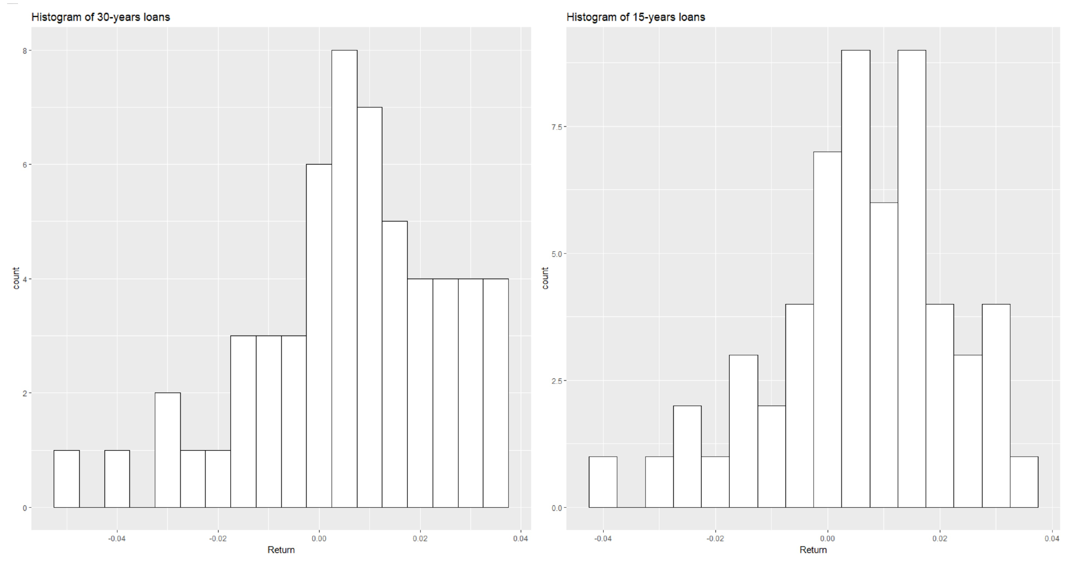
The histograms in
Figure 6 were created from the empirical distribution of the aggregated return
X. These histograms are negatively skewed in a finite interval. This is consistent with our initial assumption that the data follows PERT distribution with mode “
b” as a parameter of the distribution.
It is reasonable to fix the bounds of the interval
a and
c, and consider the mode
b as a variable parameter to analyze the sensitivity of the three leverage levels above with respect to
b. i.e., consider the derivatives of the optimal three leverage levels with respect to
b.
Chopra and Ziemba (
1993) observed that the impact of a perturbation in mean to a Kelly type of optimal allocation is much larger than that of variance. Thus, in sensitivity analysis, we focused more on the mean which is directly related to the mode
b through (
23).
4.1. One Fixed Loan Maturity
We first consider the case that there is only one kind of loan with a fixed maturity.
4.1.1. Kelly’s Point
Let us assume that
X has a PERT distribution on
whose probability density function is given by Equation (
21). Under the assumption that
a and
c are fixed, the distribution can be characterized by
through
b. Thus, substituting
and
in Equation (
21),
Notice that the Kelly optimal point
is determined by the equation,
Taking the derivative with respect to
b in Equation (
25), we have (see
Appendix B.2 for details),
4.1.2. Approximations
Exact computation for and eluded us so far. It turns out that approximating up to the second moment is adequate in this particular application. This approximation study is based on our data and the approximation fits into the situation that the data represents. It is of course not practical to model all situations in reality. The approximation is developed under certain conditions, which can be applied to the situation that the data represents and most of the real scenarios.
Let
, then using second order Taylor’s expansion around
,
can be approximated by
. Then taking the expectation of
,
is given by:
Kelly’s original utility function is the expectation of the log while our approximation model is a quadratic function which is concave but not strictly monotone. Fortunately, the monotonicity is only lost after the function reaches its maximum, whereas the interesting leverage levels are all reached before the maximum. This approximation works best when
for all
. Notice that
for
so that
and
, for all
. Thus, the approximation is a suitable method for the allocation sizes
and
as this follows
Vince and Zhu (
2015) results. The accuracy of these two allocations using the approximation is high when compared with the actual numerical computation.
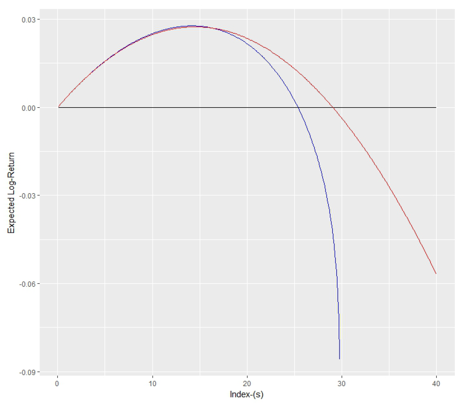
Figure 7 shows the comparison of the two curves. The expected log-return curve is almost symmetrically concave and closer to the approximate curve if the distribution is symmetric as in the diagram. The lower curve is the approximate curve and the upper curve is the expected log-return curve. Moreover, the skewness of the distribution makes the right side (after the maximum) of the log return curve steeper. Every time, the deviation of approximate curve happens around the maximum point, but before it, they are almost identical. This also shows us the approximations for
and
are accurate.
If the distribution is more skewed, then the two graphs in
Figure 7 also significantly deviate from one another. The more skewness, the more deviation. Therefore the approximation works best when the distribution of the return is almost symmetric as in our scenario. Since our analysis is based on the PERT distribution, we will find out the conditions for
b (mode) where this analysis is valid.
Table 3 presents the third moment of the random variable and the skewness of the distribution of the historical data. It shows that the third moment is very small and therefore, it is reasonable to ignore the terms beyond the third moment in the approximation.
The existence of
satisfies the inequality:
This implies equivalently that:
The approximation is valid only under this condition.
4.1.3. Return–Drawdown Ratio
The return–drawdown ratio,
, is determined by Equation (
28). It also depends on
Q, therefore the notation
is introduced here. It follows from the definition that
satisfies:
Taking derivative w.r.t
in Equation (
28) gives Equation (
A6) and simplifies to:
as in the
Appendix B.3.
4.1.4. Inflection Point
The inflection point is derived by solving Equation (
4). Approximately,
Then
can be given as:
Then, as noticed from the relationship in the numerical simulation,
is true. Now, calculate the derivative of
w.r.t
:
The discussion in the above three sections has shown that all three optimal points of leveraging increase as the mode of the distribution increases. The distribution of returns may take negative values as well. Therefore, there is a probability of losing your investment. The investment size should not exceed the capital on hand, i.e., for all . This shows us we should not increase our investment size, , beyond the limits as discussed before. These limits provide guides for the investors to not lose more than what investors have on their hand as capital. To avoid this danger, there should be limits for increasing as well as the other two leverage levels.
This whole discussion is based on an approximation, so we will carry out a sensitivity analysis (by numerical simulation) in
Section 4.2 to verify what we observe here by using an approximation.
4.2. Simulation Study
To show the approximation gives a reliable analysis, we created a random sample of returns from a PERT distribution and calculated these three optimal points using 100 different random samples by changing the mode b. For each b, we calculated three optimal points 100 times, creating 100 different random samples. Then we considered the means of all 100 for a particular b.
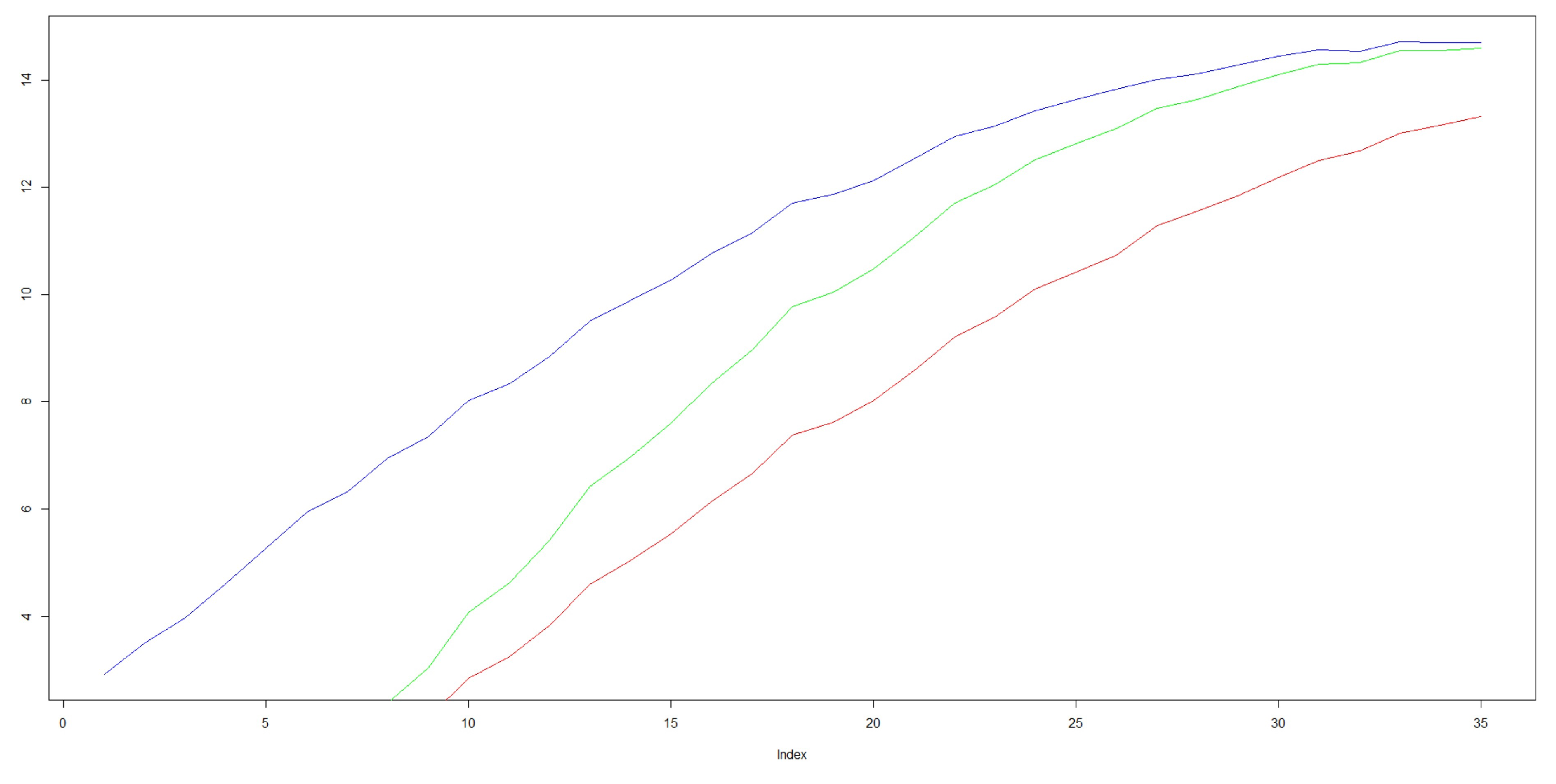
The graph in
Figure 8 shows the result for three optimal points when changing
b with the simulation described above.
Figure 9 shows how
point and
are increasing functions of
b with the bounds of
b described in the previous section.
4.3. Mixed of Loan Maturities in One Model
Next, we discuss the general situation where we consider all types of loans available together as a portfolio. Assume that the allocation proportion is
for each loan with maturity
i. Assume there are
k different types of loans. Then define the total loan balance as follows. Denote
as the duration for the loan maturity of the
loan and
l as the total size issued in every year, which is the same for each year. Then,
Then the total return is:
where,
Similar to as in single loan, the new random variable of return would be:
The effect on
, and
is similar when interest rates change. Therefore the effect on the denominator is approximately constant when interest rates change. The differences of
and
approximately cancel off the change of effects. Therefore it is reasonable to assume that
is approximately linear w.r.t
:
where:
Kelly’s point gives the solution to the following equation for (approximation)
s.
Taking the derivative of Equation (
43) w.r.t
,
As in the above equation, Equation (
44) can be used to estimate the change of
w.r.t
.
The optimal return–drawdown ratio is given by solving the following equation:
Taking derivative w.r.t
, after cancellations and replacement with estimates,
After substituting approximations and solving for
,
The inflection point is given by solving:
Taking the derivative w.r.t
, then replace with estimation,
After substituting approximate derivatives of
l,
4.4. Banker’s Strategies
We applied the above analysis to the case that there are two loans of duration, 15-year and 30-year, respectively. The results on
Table 1 and
Table 2 show that the 15-year loan is safer than 30-year loan in the sense that it has lower risk. Therefore, when interest rates increase we can increase the allocation for the 15-year loan and transfer those amounts, decreasing the allocation of the 30-year loans. Therefore, there are two options that banks can do when interest rates rise:
To affect the change of leverage size with reallocation the total derivative has to be zero. For example, in the case of Kelly’s point, one solves the following equation:
where
and
to determine the changes on allocation. Since there are only two different maturities of loans the corresponding changes of
and
can be found easily from above equation.
Consider the 15-year and the 30-year loan maturities. Then we only have two allocation sizes, which satisfy:
Then we find the percentage of change in the Equation (
51), which is a linear relationship between
and
.
The regression coefficient of average return (vs. Fed interest rates) shows that, on average, when interest rates increase by
% then the average return decreases by
. For example, if the allocation sizes start with 50% on each maturity, then the allocation change for a 15-year loan (if we use inflection point) for a 50-year investment horizon is
(
Table 4) per 0.25% increase of Fed fund rates. That means that when Fed interest rates increase by 0.25%, then the new allocation for a 15-year loan should be
% and for a 30-year loan, it should be
%
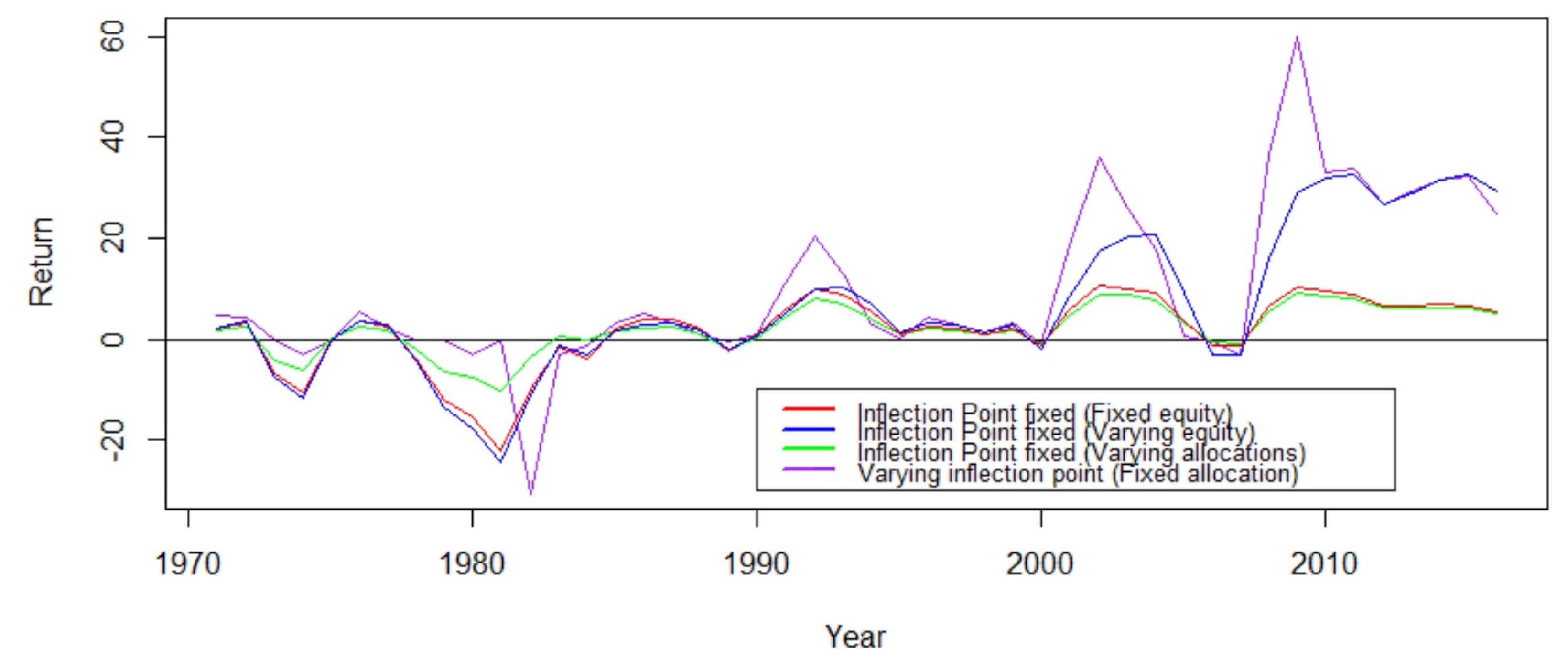
4.5. Mixed-Model: Performance Test
Varying Equity
Figure 10 shows how equity changes when using a constant leverage level. We see that
point almost causes bankruptcy during the late 1980s.
Fixing Equity
Figure 11 shows the return when changing the optimal leverage levels when Fed interest rates change. The
point again causes the highest loss during the peak of Fed interest rates in the 1980s except at 1982. This is because
is too sensitive to change according to interest rates change. Also, we noticed that in the peak points of return curve inflection point gives a higher return than return–drawdown ratio.
In the above case we have seen that inflection point performs better in terms of risk-adjusted return. Therefore, next we will compare the inflection point with different strategies.
Figure 12 shows that changing the total leverage level while fixing the allocation yields a higher return. On the other hand, fixing total leverage level and changing the allocation between loans of different maturities yields lower risk.
5. Conclusions
Testing the growth optimal leverage level (Kelly’s point) on the US mortgage market using historical data leads to almost bankruptcy during the period of 1970–1980, when the short-term interest rate was rapidly increased. The other two are more conservative compared to the Kelly point, with the inflection point as the most conservative among the three. Testing on the same historical data of the US mortgage market with 15- and 30-year fixed rate mortgages showed that both and suggest acceptable levels of leverage. Moreover, backtests on historical data also show that the 15-year loan was more favorable in producing better risk-adjusted returns when compared to the 30-year loan.
When the short-term loan interest rate was rising, the cost of financing long-term mortgages increased too, which chips away the profit margin. By sensitivity analysis we approached an important issue: The adjustment of the loan portfolio to mitigate such risks. Our sensitivity analysis qualitatively showed that the three leverage levels , , and are positively correlated to the return. Furthermore, using regression analysis on historical market data showed that the return was negatively correlated to the short-term interest rate. This means that the bank should reduce the loan portfolio leverage in an environment when the short-term interest rate was increasing and increase leverage level when the short-term interest rate was decreasing. Possible adjustments of the loan portfolios include the adjustment of the leverage level or the adjustment of the allocation into the mix of the 15-year and 30-year loan. The derivative of the point was too large to be stable in practice. On the other hand, the derivative of the point was more reasonable. Indeed, the simulation on historical data showed that adjusting either the leverage level or fixing the leverage level according to the aggregated data yielded better results compared to fixing at the level suggested by the aggregated data and adjusting the allocation between the 15-year and 30-year loan, but the later strategy lowered the risk. Based on our analysis we believe that is a reasonable leverage level for banks mortgage operations. Moreover, adjustment strategies are suggested for the loan operation to deal with different monetary policy environments.
While our analysis provided a new framework to analyze the appropriate level of loan leverages, the analysis was idealized in assuming that the empirical data rich enough to conduct estimates or calibrate the PERT distribution. The sensitivity analysis relied on an approximation using the moments up to the second order. More importantly, in practice a loan portfolio is not liquid. Changing the leverage levels or the allocation is either costly or time consuming. These are important directions for further investigation.


