Contingent Convertible Debt: The Impact on Equity Holders

Abstract

Contingent Convertible (CoCo) is a hybrid debt issued by banks with a specific feature forcing its conversion to equity in the event of the bank’s financial distress. CoCo carries two major risks: the risk of default, which threatens any type of debt instrument, plus the exclusive risk of mandatory conversion. In this paper, we propose a model to value CoCo debt instruments as a function of the debt ratio. Although the CoCo is a more expensive instrument than traditional debt, its presence in the capital structure lowers the cost of ordinary debt and reduces the total cost of debt. For preliminary equity holders, the presence of CoCo in the bank’s capital structure increases the shareholder’s aggregate value.

1. Introduction

The 1988 Basel accord ties bank capitalization to portfolio risk by introducing the Capital Adequacy Requirement (CAR). Subsequently, Basel II obliges banks to maintain sufficient loss-absorbing capital on an annual basis. However, several studies on the 2008 financial crisis, such as Flannery (2014) and Duffie (2010) reveal that, in practice, regulators are unable to force banks to maintain adequate loss-absorbing capital. To alleviate banks under-capitalization, Flannery (2005) introduced Contingent Convertibles, hereafter referred to as CoCo in accordance with most of the main-related studies. CoCo is a hybrid debt with a specific clause stipulating that the issuer would either convert it to equity or write down its face value if the level of loss-absorbing capital falls below a certain threshold. This is supposed to help with a firm’s recapitalization under distress, while equity holders would be reluctant to raise capital voluntarily by issuing new shares. Basel III recommends large financial institutions to issue CoCo as a part of their capital adequacy requirements (CAR).

CoCo carries two major risks: the risk of default, which threatens any type of debt instrument, plus the exclusive risk of mandatory conversion. CoCo differs greatly from a traditional convertible bond, which the conversion is optional and generally rewards the bondholder; hence, it is not a risk. Mandatory conversion of CoCo is a punishing mechanism which decreases the value of the bondholder in most scenarios; hence, it is a risk factor.

Most literature employs the structural approach to model CoCo dynamics. Studies generally define a trigger threshold as the barrier, then calculate the conditional probability of hitting the barrier. What makes this group of studies different is the choice of underlying instrument that triggers the conversion and the dynamics of the underlying trigger. The trigger is the book-equity-to-book-asset ratio in Glasserman and Nouri (2012), where they model the book asset process using a geometric Brownian motion (GBM). Conversion occurs if the book-equity-to-book-asset ratio exceeds a predetermined exogenous ratio. Chen et al. (2013) use the same underlying instrument while they model the book asset process using a jump-diffusion. Conversion is triggered if the asset value goes over a predetermined exogenous threshold. In Brigo et al. (2015), firm asset value is a GBM process and the conversion barrier is a linear function of the asset-to-equity ratio. De Spiegeleer et al. (2017), in a more recent study, come closer to the Basel III accord and define the implied Common Equity Tier 1 (CET1) volatility as the conversion trigger while modelling the CET1 capital ratio as a GBM. Structural modelling based on a GBM makes the conversion time predictable, while being counterfactual. Uncertainty with respect to the conversion is due not only to the use of accounting capital ratio as the conversion trigger, but also to the stipulations in Basel III that allow regulators to choose the conversion time at their discretion. Studies such as Albul et al. (2013) and Hilscher and Raviv (2014) model the CoCo as a contingent claim on the value of the bank’s assets. The results are relatively tractable models in which the bank’s incentive to issue CoCo voluntarily could be examined. Once again, the main challenge of these approaches is in triggering the conversion by the unobservable market value of assets.

In Cheridito and Xu (2015), the CoCo price is modelled using a pure reduced form approach where the conversion and default events are modelled with a time-changed Poisson process. However, the reduced form approach is less intuitive by ignoring the link between the capital ratio and the trigger event (Brigo et al. 2015). Chung and Kwok (2016) use a structural approach to model the conversion when the capital ratio falls below a certain threshold and also use a Poisson process to model the potential unexpected conversion imposed by the regulator.

Conversion price is also a matter of debate in the literature. As a basic design, Flannery (2005) proposes that the number of shares received by CoCo holders at conversion is determined by the face value of the CoCo bonds divided by the market price of stock on the day of conversion. However, this basic conversion mechanism gives an opportunity to short sellers to bid down the share price, force conversion and dilute the market by increasing the number of outstanding shares. To avoid share price manipulation, Duffie (2010) argues that the number of shares should be based on a multi-day average of closing prices. Other studies such as Flannery (2016) and Pennacchi (2010) propose converting the CoCo into a predetermined number of shares at a fixed price. However, there is a high risk that CoCo investors will suffer some value losses upon conversion due to a jump in the market price of shares.

Regulators insist that the CoCo conversion trigger should be based on the accounting capital ratio. Indeed, this is determined by the Basel Committee on Banking Supervision (BCBS) at a global level in Basel III, the European Banking Authority through the Capital Requirements Directive IV/Capital Requirements Regulation (CRD IV/CRR) and the Office of the Superintendent of Financial Institutions (OSFI) in Canada through the Capital Adequact Requirements (CAR) guidelines. The Common Equity Tiers 1 (CET1) should not fall bellow a certain percent of risk-weighted asset (RWA). Although accounting measures are not forward looking and can be manipulated by managers, they ensure that CoCo conversion occurs when a firm encounters serious financial problems. Glasserman and Nouri (2012) and Chen et al. (2013) choose asset book value as the trigger through the book-equity-to-book-asset ratio, claiming that the book asset value truly approximates the market asset value. Many studies are against employing book value as a basis of conversion because it generates a delayed signal of financial distress. McDonald (2013) and Bolton and Samama (2012) assume that the market price of equity can measure a bank’s loss-absorbing capacity. They propose a CoCo design in which the share price functions as the conversion trigger. Sundaresan and Wang (2015) point out two shortcomings of employing the market price of shares as the conversion trigger within their framework, both of which are linked to the fact that CoCo conversion generates a value exchange between CoCo holders and initial equity holders. First, if the value is transferred from shareholders to CoCo investors at conversion, there can be more than one rational expected equilibrium price for both the stocks and CoCos. Second, if the value is transferred to shareholders, the model sometimes lacks an equilibrium share price. Sundaresan and Wang (2015) conclude that a unique competitive equilibrium exists if the conversion does not induce a value transfer. Glasserman and Nouri (2012) maintain that this multiple equilibrium problem is a feature of discrete-time models and can be alleviated in a continuous time framework.

Closer to our paper, Chen et al. (2017) study the design and incentive effects of contingent convertible debt on optimal capital structure. The asset value is modelled as a jump diffusion, default and conversion occur whenever the firm value triggers some critical value. The default threshold is determined by the equity holder in such a way to maximize the equity value. They conclude that equity holders often have a positive incentive of issuing CoCos because the presence of CoCos reduces the bankruptcy costs when the conversion trigger is large enough.

In this paper, we also study the impact of having a contingent debt instrument in the debt structure in the perspective of equity holders. Based on a discrete time dynamic optimization approach, we reach similar conclusions as Chen et al. (2017). Indeed, our framework differs from the latter in various ways. First, the endogenous floating coupon rates of the standard and the CoCo debts account for the indebtedness of the firm. Second, the number of shares received by CoCo debt holders at conversion time is also designed differently. In our study, the optimal dividend stream is solved through a dynamic optimization approach: the equity holders have an incentive to control the firm debt ratio to maximize their share of the firm equity value, avoiding the dilution effect caused by conversion. It also benefits the bondholder as its mitigates the default risk.

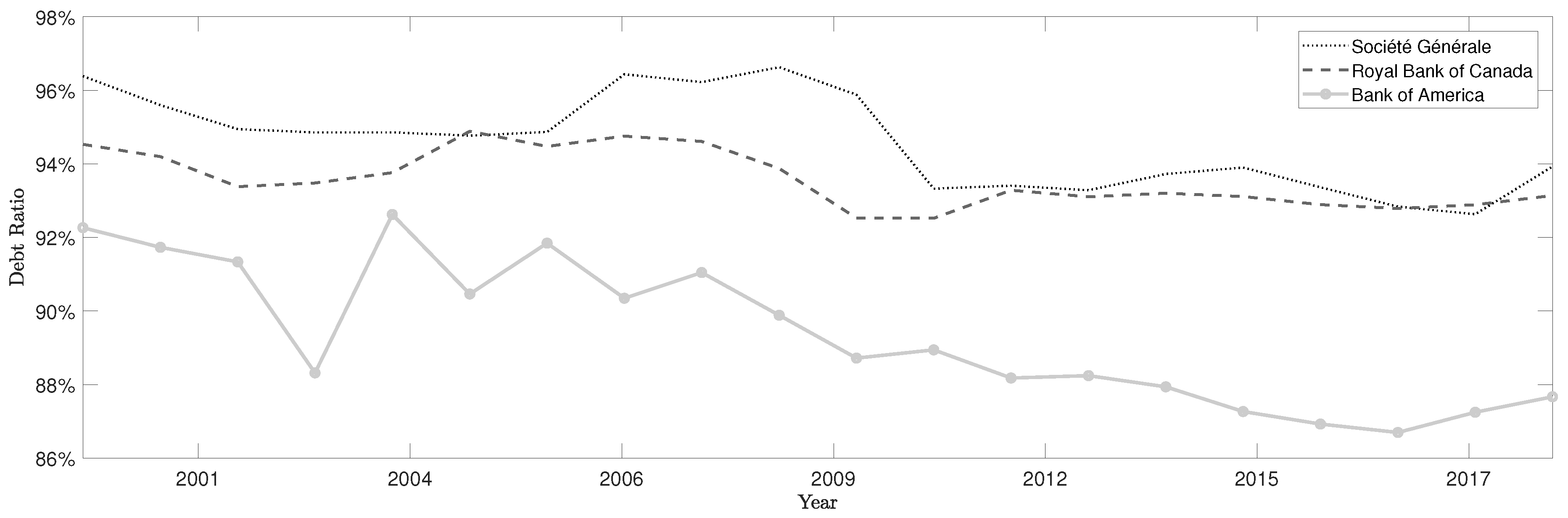
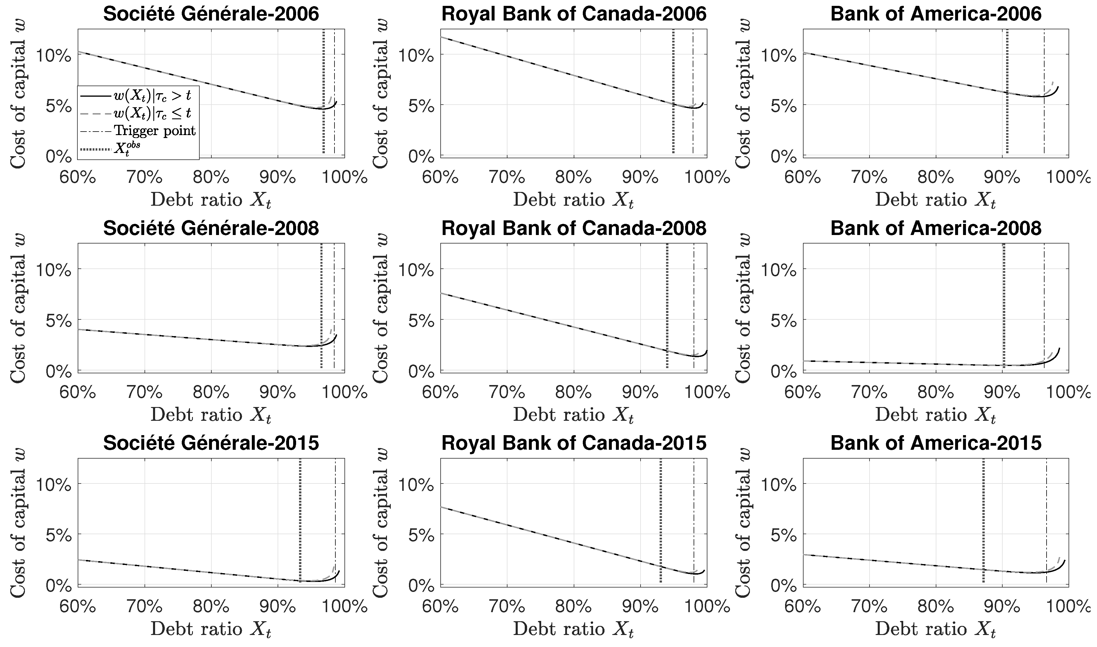
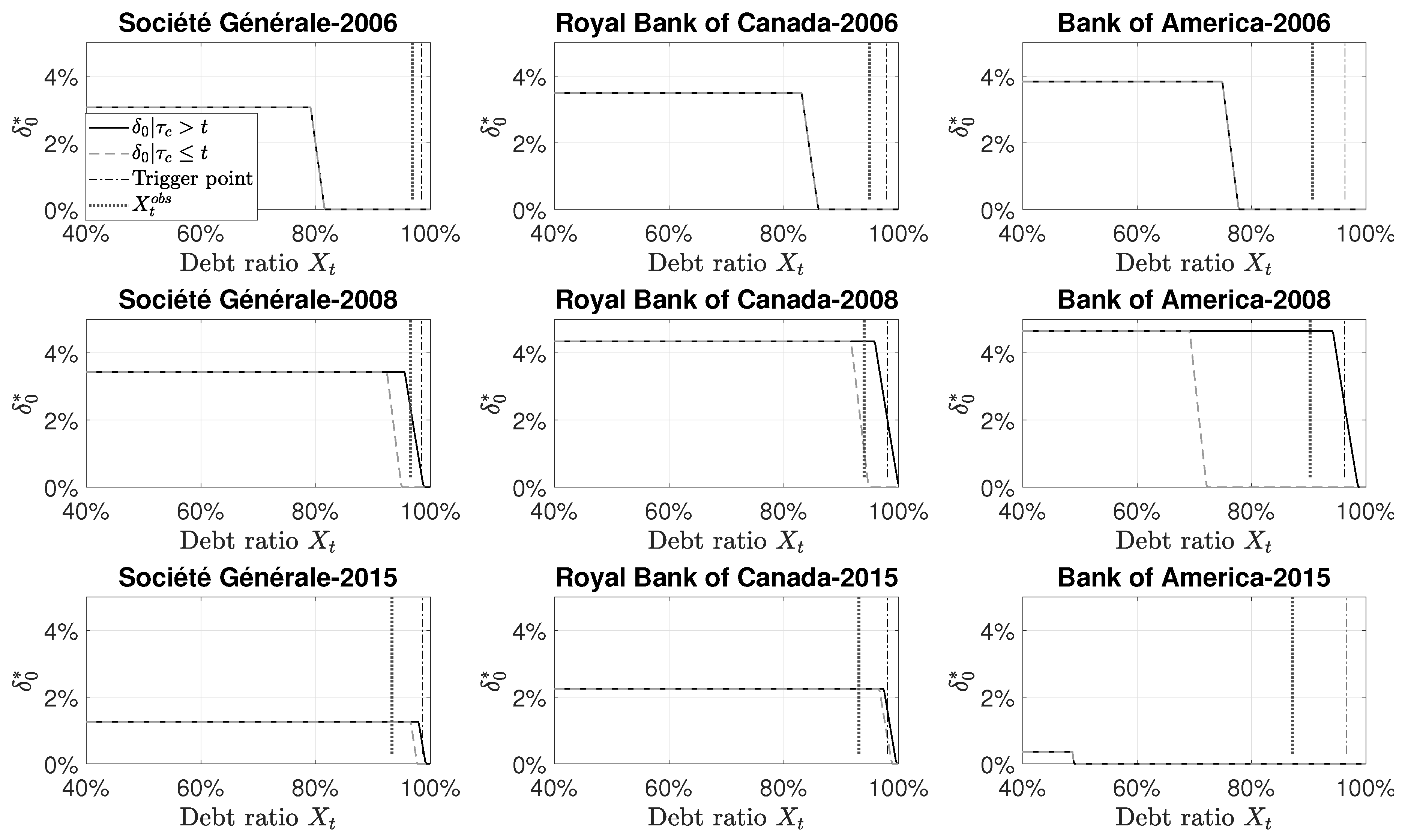
A numerical simulation based on realistic data evaluates the benefits and the costs of having CoCos in the bank’s debt structure. The parameters are estimated using three banks from three different regions (Europe, Canada and the United States), for three different periods of time (pre-crisis, crisis, post-crisis). The results help to understand how CoCos can help “Too big to fail” banks in different economic conditions. Although there are important differences among these three cases, common behaviours are observed: the presence of CoCos in the debt structure reduces the probability of default, the coupon of the standard debt, the cost of debt and capital. However, the CoCo is a more expensive instrument than the standard debt, mainly because the investor bears more risk. This study contributes to the literature by evaluating the effectiveness of adding CoCos to the financial firm’s capital structure. We do not only evaluate the CoCo debt itself, but also examine its impact on the firm’s management strategy by optimizing the per-share value of the cumulated dividend stream. Equity holders modify the optimal dividend policy to account for the conversion risk that affect them through the dilution effect (after conversion, there are more equity shares).

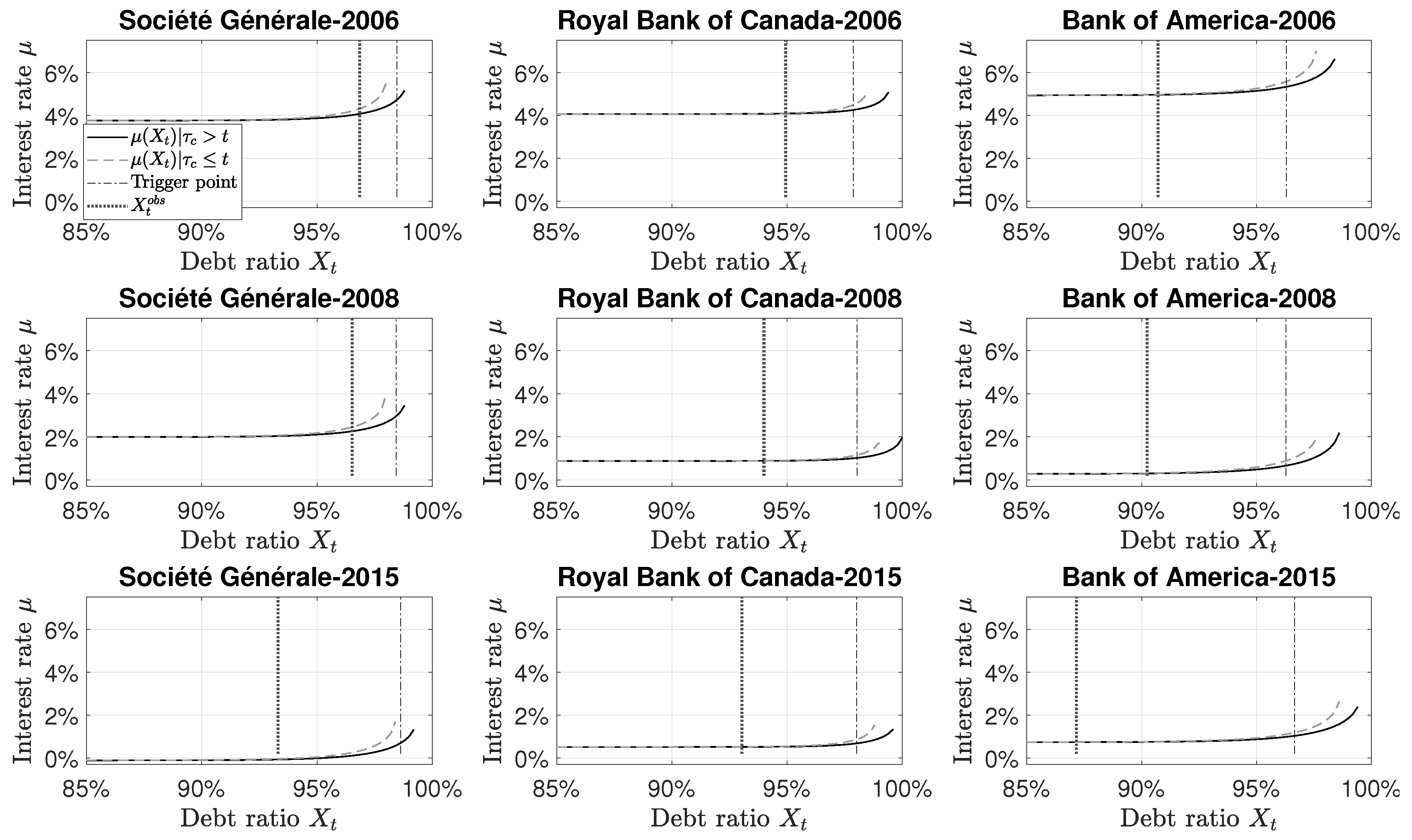
This paper is structured as follows. Section 2 presents the model to value CoCo and defines the conversion as well as the default intensity. Section 3 presents the dynamic programming model use to examine how CoCo impact the firm’s management strategy. Section 4 is decomposed into three parts. First, the data used to have realistic scenarios are presented. Second, the results are presented for each bank and each year. Third, a sensitivity analysis follows. Section 5 presents conclusions.

2. The Model

The asset value satisfies

$$A_t=E_t+D_t,$$

(1)

where $E_t$ and $D_t$ are the equity and debt values, respectively. The debt is decomposed into three main components: the deposit whose time t value is $F_t$, the coupon-paying bonds and other debt instruments for a value of $B_t,$ and a convertible contingent instrument (CoCo) whose value is $C_t$:

$$D_t=F_t+B_t+C_t.$$

The debt ratio is defined as

$$X_t=\frac{D_t}{A_t}.$$

(2)

The presence of the CoCo debt alleviates the default risk since, in case of financial distress, the CoCo debt is converted into equity, leading to a smaller debt ratio. CoCo debt holders bear not only a default risk, but also a conversion risk; therefore, they require compensation in the form of a coupon payment that differs from that of a standard debt, which is subject only to credit risk. More precisely, once converted into equity, the CoCo debt has a zero recovery rate in case of default. However, if the firm survives after the conversion, then it is not clear whether the proportion of equity value held by the CoCo debt holders will be more or less profitable than for a standard debt.

The default time is denoted ${\tau }_D,$ and the conversion time satisfies ${\tau }_C=min\left({\tau }_{\alpha },{\tau }_D\right)$, which means that the CoCo debt is always converted before the default event. Because other factors may influence the conversion decision, it does not necessarily occur as soon as the leverage ratio triggers $\alpha$, but it is very likely to occur. Consequently, the conversion intensity driving ${\tau }_{\alpha }$,

$$G_t=g\left(X_t\right)={\left(\frac{X_t}{{\theta }_C}\right)}^{{\beta }_C},$$

is a positive and convex function of $X_t$, taking large values whenever $X_t$ is above ${\theta }_C\in \left(0,1\right]$ and small values otherwise. ${\theta }_C$ should be close to $\alpha$. The parameter ${\beta }_C$ is usually a large positive constant. Therefore,

$${\mathbb{P}}_t\left({\tau }_{\alpha }=t\left|{\tau }_{\alpha }>t-1,{\tau }_D>t-1\right.\right)=\left[1-exp\left(-G_t\right)\right]{\mathbf{1}}_{{\tau }_{\alpha }>t-1}{\mathbf{1}}_{{\tau }_D>t-1}.$$

Intuitively, the conversion should occur whenever the leverage ratio is close to the critical level $\alpha$ determined by the regulator. If the CoCo debt still exists at time t, then the superscript $t^{-}$ denotes the pre-conversion values of the considered variables. The convertible contingent instrument is a coupon-paying bond with the floating coupon rate $c\left(X_t\right)$. At conversion, CoCo debt holders receive, in the form of equity shares, an amount equivalent to the debt’s face value $C_{{\tau }_C^{-}}$ and a fraction ${\rho }_C$ of the coupon. In other words, at conversion, the convertible debt holders receive

$$N_{{\tau }_C}=\frac{C_{{\tau }_C^{-}}\left(1+{\rho }_{C}c\left(X_{{\tau }_C-1}\right)\right)}{S_{{\tau }_C}}$$

equity shares where $S_{{\tau }_C}$ is the post-conversion price per share. Assuming that initially there were N outstanding equity shares, the post-conversion price per share becomes

$$S_{{\tau }_C}=\frac{E_{{\tau }_C}}{N+N_{{\tau }_C}}=\frac{E_{{\tau }_C^{-}}+C_{{\tau }_C^{-}}\left(1+{\rho }_{C}c\left(X_{{\tau }_C-1}\right)\right)}{N+\frac{C_{{\tau }_C^{-}}\left(1+{\rho }_{C}c\left(X_{{\tau }_C-1}\right)\right)}{S_{{\tau }_C}}}.$$

Multiplying both sides by $N+\frac{C_{{\tau }_C^{-}}\left(1+{\rho }_{C}c\left(X_{{\tau }_C-1}\right)\right)}{S_{{\tau }_C^{-}}}$ and isolating $S_{{\tau }_C}$ leads to

$$S_{{\tau }_C}=\frac{E_{{\tau }_C^{-}}}{N}=S_{{\tau }_C^{-}},$$

which implies that the price per share is not affected by the conversion. Then, the equity value becomes

$$E_{{\tau }_C}=E_{{\tau }_C^{-}}+C_{{\tau }_C^{-}}\left(1+{\rho }_{C}c\left(X_{{\tau }_C-1}\right)\right).$$

Letting

$$y_t=\frac{C_t}{D_t}\in \left[0,\gamma \right]\subseteq \left[0,1\right]$$

(3)

be the proportion of convertible debt in the total debt value. Because there are always deposits, then the convertible instrument represents less than 100% of the debt value, which implies that $\gamma <1$. The number of additional shares issued at conversion satisfies

$$N_{{\tau }_C}=N\left(1+{\rho }_{C}c\left(X_{{\tau }_C-1}\right)\right)y_{{}_{{\tau }_C^{-}}}\frac{X_{{\tau }_C^{-}}}{1-X_{{\tau }_C^{-}}}\cong N\left(1+{\rho }_{C}c\left(\alpha \right)\right)y_{{}_{{\tau }_C^{-}}}\left(\frac{\alpha }{1-\alpha }\right).$$

(4)

Proof. 

$$\begin{array}{ccc}\hfill N_{{\tau }_C}& =& \frac{C_{{\tau }_C^{-}}\left(1+{\rho }_{C}c\left(X_{{\tau }_C-1}\right)\right)}{S_{{\tau }_C}}=N\frac{C_{{\tau }_C^{-}}\left(1+{\rho }_{C}c\left(X_{{\tau }_C-1}\right)\right)}{E_{{\tau }_C^{-}}}=N\frac{C_{{\tau }_C^{-}}\left(1+{\rho }_{C}c\left(X_{{\tau }_C-1}\right)\right)}{D_{{\tau }_C^{-}}}\frac{D_{{\tau }_C^{-}}}{A_{{\tau }_C^{-}}}\frac{A_{{\tau }_C^{-}}}{E_{{\tau }_C^{-}}}\hfill \\ & =& N\left(1+{\rho }_{C}c\left(X_{{\tau }_C-1}\right)\right)\frac{C_{{\tau }_C^{-}}}{D_{{\tau }_C^{-}}}\frac{D_{{\tau }_C^{-}}}{A_{{\tau }_C^{-}}}\frac{1}{1-\frac{D_{{\tau }_C^{-}}}{A_{{\tau }_C^{-}}}}=N\left(1+{\rho }_{C}c\left(X_{{\tau }_C-1}\right)\right)y_{{}_{{\tau }_C^{-}}}\frac{X_{{\tau }_C^{-}}}{1-X_{{\tau }_C^{-}}}.\hfill \end{array}$$

 □

The standard debt pays the floating coupon rate of $b\left(X_t,y_t\right)$ unless default occurs. Interestingly, the debt coupon is affected by the presence of the CoCo instrument because the latter mitigates both the default and recovery risks. If

$$1-z_t=\frac{F_t}{F_t+B_t}=\frac{F_t}{D_t-C_t}=\frac{1}{1-y_t}\frac{F_t}{D_t}$$

denotes the proportion of the non-convertible contingent debt value that consists of deposits, then

$$F_t=\left(1-z_t\right)\left(1-y_t\right)D_t,B_t=z_t\left(1-y_t\right)D_t\mathrm{and}{C}_t=y_t{D}_t.$$

(5)

2.1. The Debt Ratio $\mathbb{P}$-Dynamics

Assume that the firm survives up to time $t:{\tau }_D>t.$ At the beginning of the $t+1^{\mathrm{th}}$ period, the invested capital yields returns:

$$R_{t+1}=m_{t+1}+{\sigma }_{t+1}{\epsilon }_{t+1}^{\mathbb{P}},$$

where m and ${\sigma }^2$ are predictable processes and the sequence of ${\epsilon }_t^{}$ is formed with independent standard normal random variables. The information structure is provided by the filtration ${\left\{{\mathcal{F}}_t\right\}}_{t=1}^{\infty },$ where ${\mathcal{F}}_t=\sigma \left({\left\{{\epsilon }_u^{\mathbb{P}}\right\}}_{u=1}^t\right)$ is the $\sigma$-field modelling the information available at time t. Throughout the period, decisions about the convertible contingent debt conversion and the dividend payment affect the debt and debt ratio values. At time $t+1,$ free cash flow ($FCF$) is

$$FC{F}_{t+1}=A_t{R}_{t+1}.$$

The financial flow ($FF$) is decomposed into the deposit interest payment $r_{t+1}{F}_t,$ where $r_{t+1}$ is the predictable risk-free rate, the interest payment on standard and convertible debts, $b\left(X_t,y_t\right)B_t$ and $c\left(X_t\right)C_t$ respectively, the dividend payment ${\delta }_{t+1}{A}_{t+1},$ and the debt structure variation,

$$D_{t+1}-D_t=\left(F_{t+1}-F_t\right)+\left(B_{t+1}-B_t\right)+\left(C_{t+1}-C_t\right){\mathbf{1}}_{{\tau }_C>t+1}-C_t{\mathbf{1}}_{{\tau }_C=t+1}.$$

The floating interest rates reflect the risk embedded in both standard and CoCo debts. Both types of debts contain credit risk because the firm may default. See Appendix A.

The debt structure variation is expressed as a ratio:

$${\eta }_{t+1}=\frac{D_{t+1}-D_t}{D_t}.$$

New debt issuance makes ${\eta }_{t+1}>0$, whereas debt reaching maturity or CoCo debt conversion leads to ${\eta }_{t+1}<0$.

Assumption 1.

Let $y_t=y_0{\mathbf{1}}_{{\tau }_C>t},$ where $y_0=C_0/D_0$. In other words, whenever the contingent convertible debt exists, its proportion of the total debt value remains constant.

Similarly, assuming that the proportion of deposits with respect to the non-convertible debt value remains constant over time, $\left(1-z_t\right)=\left(1-z_0\right)=F_0/(F_0+B_0)$ and $z_0=B_0/(F_0+B_0).$

Assumption 2.

At conversion time, if there is no variation in the other types of debt, then ${\eta }_{{\tau }_C}=-y_{t_C-1}.$ In the numerical implementation, we assume that ${\eta }_{t+1}=-y_t{\mathbf{1}}_{{\tau }_C=t+1}$. In other words, the debt value at conversion is modified only by the conversion of the CoCo debt to equity.

Thus, the weighted average interest rate is

$$\begin{array}{cc}\hfill {\mu }_{t+1}& ={\mu }_{t+1}\left(X_t,z_t,y_t,{\mathbf{1}}_{{\tau }_C>t+1}\right)\hfill \\ & =\left(r_{t+1}{F}_t+b\left(X_t,y_t\right)B_t+c\left(X_t\right)C_t{\mathbf{1}}_{{\tau }_C\ge t+1}\right)/D_t\hfill \\ & =r_{t+1}\left(1-z_t\right)\left(1-y_t\right)+b\left(X_t,y_t\right)z_t\left(1-y_t\right)+c\left(X_t\right)y_t{\mathbf{1}}_{{\tau }_C>t+1}.\hfill \end{array}$$

(6)

Since

$$D_{t+1}=D_t\left(1+{\eta }_{t+1}\right),$$

(7)

the financial flow satisfies

$$\begin{array}{ccc}\hfill F{F}_{t+1}& =& {\mu }_{t+1}{D}_t+D_t-D_{t+1}+{\delta }_{t+1}{A}_{t+1}\hfill \\ & =& \left({\mu }_{t+1}-{\eta }_{t+1}\right)D_t+{\delta }_{t+1}{A}_{t+1}.\hfill \end{array}$$

The bank’s profit is the difference $FCF-FF$ between the free cash flow and the financial flow. Therefore,

$$\begin{array}{ccc}\hfill A_{t+1}& =& A_t+FC{F}_{t+1}-F{F}_{t+1}\hfill \\ & =& \left(1+R_{t+1}\right)A_t-\left({\mu }_{t+1}-{\eta }_{t+1}\right)D_t-{\delta }_{t+1}{A}_{t+1},\hfill \end{array}$$

which is equivalent to

$$A_{t+1}=\frac{\left(1+R_{t+1}\right)A_t-\left({\mu }_{t+1}-{\eta }_{t+1}\right)D_t}{1+{\delta }_{t+1}}.$$

(8)

Dividing both sides of Equation (8) by $A_t,$

$$\frac{A_{t+1}}{A_t}=\frac{\left(1+R_{t+1}\right)-\left({\mu }_{t+1}-{\eta }_{t+1}\right)X_t}{1+{\delta }_{t+1}}.$$

Since

$$\frac{A_{t+1}}{A_t}=\frac{A_{t+1}}{D_{t+1}}\frac{D_{t+1}}{D_t}\frac{D_t}{A_t}=\frac{1}{X_{t+1}}\left(1+{\eta }_{t+1}\right)X_t,$$

comparing both equations and isolating $X_{t+1}$ implies that the (post-dividend) debt ratio must satisfy

$$X_{t+1}=\frac{\left(1+{\delta }_{t+1}\right)\left(1+{\eta }_{t+1}\right)X_t}{\left(1+R_{t+1}\right)-\left({\mu }_{t+1}-{\eta }_{t+1}\right)X_t}.$$

(9)

Note that

$$X_{t+1}=\left(1+{\delta }_{t+1}\right)X_{t+1}^0,$$

(10)

where $X_{t+1}^0$ denotes the pre-dividend debt ratio

$$X_{t+1}^0={\left.X_{t+1}\right|}_{{\delta }_{t+1}=0}=\frac{\left(1+{\eta }_{t+1}\right)X_t}{\left(1+R_{t+1}\right)-\left({\mu }_{t+1}-{\eta }_{t+1}\right)X_t}.$$

2.2. Conversion

The conversion decision is taken under the assumption that ${\delta }_{t+1}=0$, ${\eta }_{t+1}=0$ (no debt issuing or refunding) and that the full interest payment includes the CoCo debt coupon:

$${\mu }_{t+1}^C=r_{t+1}\left(1-z_t\right)\left(1-y_t\right)+b\left(X_t,y_t\right)z_t\left(1-y_t\right)+c\left(X_t\right)y_t.$$

(11)

The conversion intensity

$$G_{t+1}=g\left(X_{t+1}^C\right)={\left(\frac{X_{t+1}^C}{{\theta }_C}\right)}^{{\beta }_C}$$

(12)

is a positive, increasing, and convex function of the debt ratio

$$X_{t+1}^C=\frac{X_t}{\left(1+R_{t+1}\right)-{\mu }_{t+1}^C{X}_t},$$

(13)

which is a particular case of Equation (9). The parameter ${\theta }_C$ is the critical level from which the conversion probability grows fast beyond this threshold. Because of the convex relation between the conversion intensity and the conversion probability, ${\theta }_C$ is not exactly equal to the regulator critical level $\alpha$, but it is in its neighborhood. The parameter ${\beta }_C$ captures the growth speed. In the numerical implementation, both parameters are obtained through a calibration approach based on the regulator critical level $\alpha$. For this reason, ${\tau }_{\alpha }$ denotes the conversion time characterized by the conversion intensity $\alpha$. The conditional conversion probability at time $t+1$ triggered by the critical level $\alpha$ (letting ${\beta }_C\to \infty$, we recover the case where conversion occurs as soon as $X_{t^{-}}>\alpha$) is

$${\mathbb{P}}_{t+1}\left({\tau }_{\alpha }=t+1\left|{\tau }_C>t\right.\right)=\left[1-exp\left(-G_{t+1}\right)\right]{\mathbf{1}}_{{\tau }_C>t}.$$

Because immediate conversion may also arise as a consequence of an unpredicted default, the survival conversion probability is

$$\begin{array}{ccc}\hfill {\mathbb{P}}_{t+1}\left({\tau }_C>t+1\left|{\tau }_C>t\right.\right)& =& {\mathbb{P}}_{t+1}\left({\tau }_{\alpha }>t+1,{\tau }_D>t+1\left|{\tau }_C>t\right.\right)\hfill \\ & =& {\mathbb{P}}_{t+1}\left({\tau }_{\alpha }>t+1\left|{\tau }_C>t\right.\right){\mathbb{P}}_{t+1}\left({\tau }_D>t+1\left|{\tau }_C>t\right.\right)\hfill \\ & =& exp\left(-H_{t+1}{\mathbf{1}}_{{\tau }_C>t}-G_{t+1}\right).\hfill \end{array}$$

Then, the conditional conversion probability arising from both the critical level and the potential default is

$$\begin{array}{c}\hfill {\mathbb{P}}_{t+1}\left({\tau }_C=t+1\left|{\tau }_C>t\right.\right)=\left[1-exp\left(-H_{t+1}{\mathbf{1}}_{{\tau }_C>t}-G_{t+1}\right)\right]{\mathbf{1}}_{{\tau }_C>t},\end{array}$$

(14)

where the default intensity $H_{t+1}$ is defined at Equation (17).

2.3. Default

Since default occurs after conversion, the interest payment does not include the CoCo debt coupon. Indeed, a fraction of the CoCo coupon is paid back to CoCo debt holders in the form of equity shares. This means that

$${\mu }_{t+1}^D=r_{t+1}\left(1-z_t\right)\left(1-y_t\right)+b\left(X_t,y_t\right)z_t\left(1-y_t\right).$$

(15)

The default intensity is based on the pre-dividend debt ratio. More precisely, assuming that there are no dividends, ${\delta }_{t+1}=0,$ and that the only debt variation considered is the one arising from an immediate conversion, ${\eta }_{t+1}=-y_t{\mathbf{1}}_{{\tau }_C=t+1}$, the pre-dividend debt ratio is

$$X_{t+1}^D=\frac{\left(1-y_t\right)X_t}{\left(1+R_{t+1}\right)-\left({\mu }_{t+1}^D+y_t\right)X_t}{\mathbf{1}}_{{\tau }_{\alpha }>t}+\frac{X_t}{\left(1+R_{t+1}\right)-{\mu }_{t+1}^D{X}_t}{\mathbf{1}}_{{\tau }_{\alpha }\le t}.$$

(16)

Since a debt ratio augmentation has more impact on the default probability when the debt ratio is already high, the default intensity $H_{t+1}$ is a positive, increasing, and convex function of the debt ratio. More precisely,

$$H_{t+1}=h\left(X_{t+1}^D,y_t\right)={\lambda }_D+{\left(\frac{X_{t+1}^D}{{\theta }_{D,t}}\right)}^{{\beta }_D},$$

(17)

where ${\theta }_{D,t}={\theta }_D+y_t$, ${\lambda }_D\ge 0,{\theta }_D>\alpha ,{\beta }_D>1$. Indeed, ${\theta }_{D,t}$ represents the critical debt ratio from which the increasing behaviour of the default probability (seen as a function of the debt ratio) accelerates. Because the CoCo instrument provides the standard debt holders with an additional protection against default risk, the critical debt ratio is ${\theta }_{D,t}$ slightly higher whenever the CoCo debt is present in the debt structure. Consequently, the conditional default probabilities are

$${\mathbb{P}}_{t+1}\left({\tau }_D=t+1\left|{\tau }_C>t,{\tau }_D>t\right.\right)=\left[1-exp\left(-H_{t+1}{\mathbf{1}}_{{\tau }_C>t}\right)\right]{\mathbf{1}}_{{\tau }_D>t}$$

(18)

and

$${\mathbb{P}}_{t+1}\left({\tau }_D=t+1\left|{\tau }_C\le t,{\tau }_D>t\right.\right)=\left[1-exp\left(-H_{t+1}{\mathbf{1}}_{{\tau }_C\le t}\right)\right]{\mathbf{1}}_{{\tau }_D>t}.$$

(19)

3. Stochastic Optimum Control Problem

The period $\left]t,t+s\right]$ discount factor is

$$D{F}_{t,t+s}=\prod _{u=t}^{t+s-1}\frac{1}{1+w\left(X_u\right)},$$

where the cost of capital is a weighted average of the cost of equity, $r^E$, and the cost of debt:

$$w\left(X_u\right)=\left(1-X_u\right)r_u^E+X_u{\mu }_u.$$

(20)

The current equity holders want to maximize their share of dividends. More precisely, given a stream of dividend rates ${\delta }_{1:\infty }={\left\{{\delta }_i\right\}}_{i=1}^{\infty }$, the expected value of the discounted dividends at time t is

$$\begin{array}{ccc}\hfill V\left(t,X_t^0,{\delta }_{t:\infty }\right){\mathbf{1}}_{{\tau }_D>t}& =& \sum _{u=t}^{\infty }{\mathrm{E}}_t^{\mathbb{P}}\left[D{F}_{t,u}{\delta }_u{A}_u\left({\mathbf{1}}_{{\tau }_C>u}+\frac{N}{N+N_{{\tau }_C}}{\mathbf{1}}_{{\tau }_C\le u}\right){\mathbf{1}}_{{\tau }_D>u}\right]{\mathbf{1}}_{{\tau }_D>t}\hfill \\ & \cong & \sum _{u=t}^{\infty }{\mathrm{E}}_t^{\mathbb{P}}\left[D{F}_{t,u}{\delta }_u{A}_u\left(1-\frac{\left(1+{\rho }_{C}c\left(\alpha \right)\right)y_0\alpha }{1-\alpha +\left(1+{\rho }_{C}c\left(\alpha \right)\right)y_0\alpha }{\mathbf{1}}_{{\tau }_C\le u}\right){\mathbf{1}}_{{\tau }_D>u}\right]{\mathbf{1}}_{{\tau }_D>t},\hfill \end{array}$$

since Assumption 1 and Equation (4) imply that

$${\mathbf{1}}_{{\tau }_C>u}+\frac{N}{N+N_{{\tau }_C}}{\mathbf{1}}_{{\tau }_C\le u}=1-\frac{N_{{\tau }_C}}{N+N_{{\tau }_C}}{\mathbf{1}}_{{\tau }_C\le u}\cong 1-\frac{\left(1+{\rho }_{C}c\left(\alpha \right)\right)y_{{}_0}\alpha }{1-\alpha +\left(1+{\rho }_{C}c\left(\alpha \right)\right)y_0\alpha }{\mathbf{1}}_{{\tau }_C\le u}.$$

Since V allows for the decomposition

$$\begin{array}{ccc}\hfill V\left(t,X_t^0,{\delta }_{t:\infty }\right){\mathbf{1}}_{{\tau }_D>t}& \cong & {\delta }_t{A}_t\left(1-\frac{\left(1+{\rho }_{C}c\left(\alpha \right)\right)y_0\alpha }{1-\alpha +\left(1+{\rho }_{C}c\left(\alpha \right)\right)y_0\alpha }{\mathbf{1}}_{{\tau }_C\le t}\right){\mathbf{1}}_{{\tau }_D>t}\hfill \\ & & +{\mathrm{E}}_t^{\mathbb{P}}\left[D{F}_{t,t+1}V\left(t+1,X_{t+1}^0,{\delta }_{t+1:\infty }\right){\mathbf{1}}_{{\tau }_D>t+1}\right]{\mathbf{1}}_{{\tau }_D>t},\hfill \end{array}$$

(21)

the optimal dividend rate sequence ${\delta }_{1:\infty }^{\mathrm{opt}}$ can be constructed recursively using backward recursion over time:

$$\begin{array}{ccc}\hfill {\delta }_t^{\mathrm{opt}}& =& arg\underset{{\delta }_t\in \left[0,{\delta }_t^{max}\right]}{max}\left\{A_t{\delta }_t\left(1-\frac{\left(1+{\rho }_{C}c\left(\alpha \right)\right)y_0\alpha }{1-\alpha +\left(1+{\rho }_{C}c\left(\alpha \right)\right)y_0\alpha }{\mathbf{1}}_{{\tau }_C\le t}\right)\right.\hfill \\ & & \left.+{\mathrm{E}}_t^{\mathbb{P}}\left[\frac{V\left(t+1,X_{t+1}^0,{\delta }_{t+1:\infty }^{\mathrm{opt}}\right)}{1+w\left(X_t\right)}{\mathbf{1}}_{{\tau }_D>t+1}\right]\right\}{\mathbf{1}}_{{\tau }_D>t}.\hfill \end{array}$$

(22)

See Appendix D. Because $\frac{A_{t+1}}{A_t}=\frac{D_t}{A_t}\frac{D_{t+1}}{D_t}\frac{A_{t+1}}{D_{t+1}}=\frac{X_t}{X_{t+1}}\left(1+{\eta }_t\right)$,

$$\begin{array}{ccc}\hfill v\left(t,X_t^0,{\delta }_{t:\infty }\right){\mathbf{1}}_{{\tau }_D>t}& =& \frac{V\left(t,X_t^0,{\delta }_{t:\infty }\right)}{A_t}{\mathbf{1}}_{{\tau }_D>t}\hfill \\ & \cong & {\delta }_t\left(1-\frac{\left(1+{\rho }_{C}c\left(\alpha \right)\right)y_0\alpha }{1-\alpha +\left(1+{\rho }_{C}c\left(\alpha \right)\right)y_0\alpha }{\mathbf{1}}_{{\tau }_C\le t}\right){\mathbf{1}}_{{\tau }_D>t}\hfill \\ & & +{\mathrm{E}}_t^{\mathbb{P}}\left[D{F}_{t,t+1}\frac{X_t}{X_{t+1}}\left(1+{\eta }_t\right)v\left(t+1,X_{t+1}^0,{\delta }_{t+1:\infty }\right){\mathbf{1}}_{{\tau }_D>t+1}\right]{\mathbf{1}}_{{\tau }_D>t}\hfill \end{array}$$

(23)

and

$$\begin{array}{ccc}\hfill {\delta }_t^{\mathrm{opt}}& =& arg\underset{{\delta }_t\in \left[0,{\delta }_t^{max}\right]}{max}\left\{{\delta }_t\left(1-\frac{\left(1+{\rho }_{C}c\left(\alpha \right)\right)y_0\alpha }{1-\alpha +\left(1+{\rho }_{C}c\left(\alpha \right)\right)y_0\alpha }{\mathbf{1}}_{{\tau }_C\le t}\right)\right.\hfill \\ & & \left.+{\mathrm{E}}_t^{\mathbb{P}}\left[\frac{X_t}{X_{t+1}}\left(1+{\eta }_t\right)\frac{v\left(t+1,X_{t+1}^0,{\delta }_{t+1:\infty }^{\mathrm{opt}}\right)}{1+w\left(X_t\right)}{\mathbf{1}}_{{\tau }_D>t+1}\right]\right\}{\mathbf{1}}_{{\tau }_D>t}.\hfill \end{array}$$

Therefore, we work with a standardized version of the primary equity holders’ share of cumulated discounted dividends. Indeed, under this form, the dynamic optimization does not require the modelling of the dynamics of A.

The dividend rate is bounded above. Indeed, if the dividend payment is too large, the equity value will drop below its current level. More precisely, noting that $X_t=\left(1+{\delta }_t\right)X_t^0$, the expected variation of the pre-dividend equity is (see Appendix B.3)

$${\mathrm{E}}_t^{\mathbb{P}}\left[{\left.E_{t+1}\right|}_{{\delta }_{t+1}=0}-E_t\right]\le \left(m_{t+1}-\left(1+{\delta }_t\right)X_t^0{\mu }_{t+1}\left(\left(1+{\delta }_t\right)X_t^0\right)\right)A_t.$$

We restrict ${\delta }_t$, making the right-hand side bound positive. Now, let $x_0$ be the solution of $m_{t+1}-x_0{\mu }_{t+1}\left(x_0\right)=0$. Indeed, since $x\mu \left(x\right)$ is an increasing function of x starting at 0, a unique solution exists. Since equity holders do not reduce the expected equity value deliberately, it follows that

$$\begin{array}{cc}& m_{t+1}-\left(1+{\delta }_t\right)X_t^0{\mu }_{t+1}\left(\left(1+{\delta }_t\right)X_t^0\right)\ge 0\hfill \\ ⟺& \left(1+{\delta }_t\right)X_t^0{\mu }_{t+1}\left(\left(1+{\delta }_t\right)X_t^0\right)\le m_{t+1}\hfill \\ ⟺& \left(1+{\delta }_t\right)X_t^0\le x_0\hfill \\ ⟺& {\delta }_t\le \frac{x_0}{X_t^0}-1.\hfill \end{array}$$

In addition, since $\frac{x_0}{X_t^0}-1\to \infty$ as $X_t^0\to 0$, this upper dividend rate bound is not active for small debt ratio values. However, the dividend rate is generally lower than the expected asset returns, which leads to ${\delta }_t\in \left[0,{\delta }_t^{max}\right]$, where

$${\delta }_t^{max}=min\left(max\left(\frac{x_0-X_t^0}{X_t^0},0\right),m_{t+1}\right).$$

(24)

Dynamic programming optimization allows using a recursive method starting from T with backward induction. At each time period, the value function is the sum of the immediate dividend and the expected future dividend gain. To initialize the recursion, a long time horizon T is chosen for which some simplifications are made. Because the model is Markovian, after some iterations, the terminal conditions vanish and, for that reason, the following assumption has no impact on our numerical results. The algorithm stops when the variations in the optimal dividend become very small. Then, for time T, the following simplifications are to be assumed.

Assumption 3.

For any $t>T$,

1. 

The asset returns are no longer uncertain, that is, $R_t=m_T$, ${\sigma }_t^2=0;$

2. 

There is no more possibility of conversion, that is, the CoCo debt becomes a standard debt;

3. 

The dividends are the remaining part of the returns once the interest rate payment on the debts is deducted:

$${\delta }_t{A}_t=max\left(m_T{A}_t-{\mu }_t{D}_{t-1},0\right);$$

(25)

4. 

If the dividend payment $m_T{A}_t-{\mu }_t{D}_{t-1}$ is positive, then there is no variation of the debt value, that is, $D_t=D_{t-1}$ or, equivalently, ${\eta }_t=0;$

5. 

The risk-free rate $r_t$ is constant and equal to $r.$

Since a potential conversion is no longer possible (Assumption 3-2), for all $t>T$, the coupon on the CoCo debt is the same as the one on the ordinary debt, that is,

$$\begin{array}{ccc}\hfill {\mu }_t& =& r\left(1-z_{t-1}\right)\left(1-y_T\right)+b\left(X_{t-1},0\right)z_{t-1}\left(1-y_T\right)+b\left(X_{t-1},0\right)y_T\hfill \\ & =& r\left(1-z_{t-1}\right)\left(1-y_T\right)+b\left(X_{t-1},0\right)\left(1-\left(1-z_{t-1}\right)\left(1-y_T\right)\right).\hfill \end{array}$$

Assume for a moment that $m_T{A}_t-{\mu }_t{D}_{t-1}\ge 0$. As a consequence of Assumption 3-3, $\forall t>T$,

$$FC{F}_t-F{F}_t=m_T{A}_{t-1}-\left({\mu }_t-{\eta }_t\right)D_{t-1}-{\delta }_t{A}_t=0,$$

which implies that $A_t=A_{t-1}.$ Therefore,

$${\delta }_t=\frac{1}{A_t}max\left(m_T{A}_t-{\mu }_t{D}_{t-1},0\right)=max\left(m_T-{\mu }_t\frac{A_{t-1}}{A_t}\frac{D_{t-1}}{A_{t-1}},0\right)=max\left(m_T-{\mu }_t{X}_{t-1},0\right).$$

Moreover, from Assumption 3-4, $D_t=D_{t-1},$ it follows that $X_t=X_{t-1}$ and ${\mu }_{t+1}={\mu }_t.$ In addition, a recursive argument leads to the following conclusion: if the dividend rate is positive, that is

$$0\le {\delta }_{T+1}=\frac{m_T{A}_{T+1}-{\mu }_{T+1}{D}_T}{A_{T+1}}=m_T-{\mu }_{T+1}\frac{A_T}{A_{T+1}}{X}_T=m_T-{\mu }_{T+1}{X}_T,$$

then for all $t>T$, $X_t=X_T$, $A_t=A_T$, ${\mu }_t={\mu }_{T+1}$ and ${\delta }_t={\delta }_{T+1}=m_T-{\mu }_{T+1}{X}_T.$ The discount factor then becomes

$$D{F}_{t,t+s}=\prod _{u=t}^{t+s-1}{(1+w(X_T))}^{-1}={\left(1+w\left(X_T\right)\right)}^{-s}.$$

If $m_T{A}_t-{\mu }_t{D}_{t-1}<0$, then not only is there no dividend payment, but also the firm needs to issue more debt to cover the interest expenses: $D_t=D_{t-1}+{\mu }_t{D}_{t-1}-m_T{A}_t.$ In that case,

$$\begin{array}{ccc}\hfill F{F}_t& =& {\mu }_t{D}_{t-1}+D_{t-1}-D_t\hfill \\ & =& {\mu }_t{D}_{t-1}+D_{t-1}-D_{t-1}-{\mu }_t{D}_{t-1}+m_T{A}_t\hfill \\ & =& m_T{A}_t\hfill \\ & =& FC{F}_t\hfill \end{array}$$

and $A_t=A_{t-1}+FC{F}_t-F{F}_t=A_{t-1}.$ Therefore, the debt is growing and the asset value is stable, which implies that the debt ratio will increase until default.

Lemma 1.

Under Assumption 3, the expected value of the discounted dividends at time T satisfies

$$\begin{array}{cc}& V\left(T,X_T^0,{\delta }_T\right){\mathbf{1}}_{{\tau }_D>T}\hfill \\ \cong & A_T\left(1-\frac{y_0\alpha }{1-\alpha +y_0\alpha }{\mathbf{1}}_{{\tau }_C\le T}\right)\left\{{\delta }_T+{\delta }_{T+1}\left(\frac{exp\left(-h\left(X_T\right)\right)}{1+w\left(X_T\right)-exp\left(-h\left(X_T\right)\right)}\right)\right\}{\mathbf{1}}_{{\tau }_D>T},\hfill \end{array}$$

(26)

where ${\delta }_{T+1}=m_T-{\mu }_{T+1}{X}_T$, $h\left(X_T\right)={\lambda }_D+{\left(\frac{1}{{\theta }_D}max\left(X_T;0\right)\right)}^{{\beta }_D}$ and $X_T=\left(1+{\delta }_T\right)X_T^0.$

See proof in Appendix B.4.

4. Numerical Results

To generate realistic scenarios, the parameters correspond to the financial ratio of three banks in three different countries (Europe, Canada and the United States). The aim is to analyze how “too big to fail” banks can react in the case where there is or not CoCo in the debt structure. We focus the analysis on three different periods corresponding to the pre-crisis (2006), the crisis (2008) and the post-crisis (2015).

4.1. Data

The sample is composed of three banks listed as Global-Systemically Important Banks (G-SIBs): Société Générale for Europe, Royal Bank of Canada for Canada and Bank of America in the United States. For each bank and for each year, the debt ratio is calculated from Equation (2). The total amount of asset ($A_t$), deposit ($F_t$), long and short-term debt ($B_t$) and CoCo ($C_t$) are obtained using Bloomberg (Bloomberg Financial Analysis and Bloomberg Contingent Convertibles Search).

Figure 1 shows the evolution of the debt ratio over time, according to the banks. The French bank has the highest debt ratio during the financial crisis of 2008. Nowadays, the French and the Canadian banks appear to have the same level of debt in their financial structure. The decomposition of the debt structure, as presented in

Table 1. Source of assets.

	Société Générale	Royal Bank of Canada	Bank of America
Equity/Asset	5.41%	6.43%	10.62%
Deposit/Asset	40.60%	77.37%	58.86%
Bonds (including CoCo)/Asset	53.99%	16.20%	32.52%

The table presents the average of three financial ratios over 19 years, from 1999 to 2018. Asset is computed using Equation (1). Deposit, Equity and Bonds (including CoCo) are based on the financial statement available on Bloomberg.

, bring out that the French bank finance these activities with fewer deposit and more bonds than the Canadian and U.S. Bank.

CoCo was first launched in Europe at the end of 2009, after the financial crisis, to fulfill a need in terms of risk management. CoCos appear as a potential solution to absorb losses when the capital of banks fall below a certain level. CoCos issuance has started to rapidly increase since 2013/2014: under Basel III, certain specific CoCos are categorized as additional Tier 1 Capital (AT1). Nowadays, CoCos throughout the world are mainly issued by European and Asian companies. Canadian banks started to issue CoCos in 2014 while American banks do not.

To initialize the dynamic optimization, the percentage of CoCos in the debt structure is assumed to be $1\%$, since it is quite representative of the European and Canadian banks. Indeed, based on the debt value and the amount of CoCos issued by banks, obtained from Bloomberg, the percentage of CoCos in the debt structure is around $1.15\%$ for European banks and around $0.64\%$ for Canadian banks. For the American bank, assuming $1\%$ of CoCos could shed light on how it could help the bank in case of financial distress.

Table 2. Parameter values of the dynamic optimization per bank per year.

	Société Générale			Royal Bank of Canada			Bank of America
	2006	2008	2015	2006	2008	2015	2006	2008	2015
Returns
$r_t$	$3.76\%$	$1.99\%$	$-0.2\%$	$4.07\%$	$0.89\%$	$0.51\%$	$4.94\%$	$0.28\%$	$0.73\%$
$r_t^E$	$20.04\%$	$7.02\%$	$6.23\%$	$23.21\%$	$17.64\%$	$18.42\%$	$18.07\%$	$1.81\%$	$6.27\%$
m	$3.07\%$	$3.43\%$	$1.26\%$	$3.5\%$	$4.35\%$	$2.25\%$	$3.84\%$	$4.66\%$	$0.36\%$
${\sigma }^2$	$2\%$			$2\%$			$2\%$
Initial debt structure
$F_0$	$31.41\%$	$29.71\%$	$44.35\%$	$79.58\%$	$86.39\%$	$83.45\%$	$54.78\%$	$56.13\%$	$70.29\%$
$y_0$	$1\%$			$1\%$			$1\%$
Conversion risk
$\alpha$	$98.47\%$	$98.43\%$	$98.63\%$	$97.86\%$	$98.03\%$	$98.03\%$	$96.30\%$	$96.28\%$	$96.65\%$
${\beta }_C$	$74.48$			$66.55$			$39.85$
${\theta }_C$	$97.42\%$			$96.82\%$			$94.69\%$
${\rho }_C$	$90\%$			$90\%$			$90\%$
Default risk
${\theta }_D$	$107.7\%$			$104.11\%$			$107.29\%$
${\beta }_D$	$47.2$			$69.9$			$40.46$
${\lambda }_D$	0			0			0
${\rho }_D$	$0.4$			$0.4$			$0.4$
Numerical scheme
T	30			30			30
${\Delta }_x$	$0.002$			$0.002$			$0.002$
${\Delta }_t$	1			1			1

$r_t$ stands for risk-free rate and correspond to the one-year zero coupon curve computed by each central bank of each region. $r_t^E$ stands for the Return on Equity. m stands for the average of the expected return on capital and ${\sigma }^2$ its variance. $F_0$ means the percentage of deposit at time 0. $y_0=C_0/D_0$ is the initial proportion of CoCo debt. The conversion and default intensities functions are respectively Equations (12) and (17). The debt ratio mesh parameter ${\Delta }_x$ represents the distance between two consecutive debt ratios. The time discretization is ${\Delta }_t=1$ year.

presents the parameter values obtained from the financial ratio of three banks, for three different periods corresponding to the pre-crisis (2006), the crisis (2008) and the post-crisis (2015). The critical debt ratio parameters (${\theta }_C$ and ${\theta }_D$) and the convexity parameters (${\beta }_C$ and ${\beta }_D$) characterizing the conversion and default intensities were obtained by calibrating the conversion and default probabilities (more details in Appendix C). The results obtained for the critical debt level of the conversion intensity ${\theta }_C$ is near 95%. This is due to the fact that, under Basel III, CoCos that have a minimum trigger level of $5.125\%$ in terms of Common Equity Tier 1 by risk-weighted assets and having perpetual coupons are qualified as additional tiers 1. Previously, there had been a trend towards issuing CoCos with such characteristics. This corresponds to a trigger level imposed by the regulator ($\alpha$) in terms of debt ratio close to 1–5.125% of risk-weighted assets. The critical debt ratio of the default intensity obtained, ${\theta }_D$, is slightly greater than $100\%$. When a firm has more liabilities than assets, there is a high risk of insolvent and excess leverage. The convexity conversion (default) parameter, ${\beta }_C$ (${\beta }_D$), is designed to increase the conversion probability (default probability) rapidly around the critical debt ratio ${\theta }_C$ (${\theta }_D$). This leads to high convexity parameters.

The credit risk management literature suggests that the recovery rate is around $40\%$, based mainly on observed data (Altman and Kishore 1996; Duffie and Lando 2001). The risk-free rate corresponds to the one-year zero coupon curve computed by the European Central Banking, Bank of Canada and the Federal Reserve Bank of St. Louis. $r_t^E$ corresponds to the Return on Equity (ROE). m is the expected capital return expected by investors and is therefore not directly observable. We have chosen to proxy $m_t$ by the average ROE over the last five years and the average risk-free rate, such that $m_t=(1-x){\overline{r}}_t^E+x{\overline{r}}_t$.

4.2. Empirical Results

Using the parameters presented in Table 2, Equations (14), (18) and (19) are used to compute the one-year conversion probability and the one-year default probabilities as a function of the actual debt ratio. Figure 2 shows that, for each bank and for each year, the conversion probability increases with the debt ratio. Around the debt ratio critical level, the conversion probability tends to climb to $100\%$ reflecting the mandatory conversion. As expected, the presence of CoCo debt instruments reduces the default probabilities. When there is no more CoCo in the debt structure, the default probability increases more rapidly. It confirms that having CoCos in the debt structure acts like a safety buffer. The conversion and default probabilities are not only driven by the intensity parameters, but also by the actual market conditions, that is, the risk-free rate, the expected return on the capital, and the debt structure. Figure 2 shows that the probabilities of default were greater in 2006, with more indebted banks.

Equations (A4)–(A6) give the coupon rate on the standard debt (with and without CoCos) and the CoCo debt. CoCo debt holders face two risks: the risk of default (like the standard debt holders), plus the risk of mandatory conversion. However, since at conversion, CoCo debt holders receive in terms of equity the value of their investment, there is no conversion recovery risk. Figure 3 shows that when the contingent debt is present in the debt structure, the CoCo debt is more expensive than the standard debt. Moreover, as the contingent debt mitigates the default risk, the coupon rate of the ordinary debt is notably lower in the presence of CoCos. Comparing the result for each bank and each year, Figure 3 shows that the coupons are lower over the years due to lower interest rate. The risk-free rates were higher before the financial crisis and stayed at low levels after the crisis.

The cost of debt (Equation (6)) is a weighted average of each component (deposit, standard debt and CoCo debt). Figure 4 shows that the cost of debt increases for large debt ratio which is a direct consequence of the coupon curve behavior (Figure 3). Even if the CoCo coupon rate is large relatively to the standard debt coupon rate, for high-debt ratio, the presence of CoCo in the debt structure reduces the cost of debt. Over the years, the cost of debt decreases, mainly due to the lower risk-free rate. Because Royal Bank of Canada uses mainly deposits over bonds, the cost of debt is not so much affected by the increase in the coupon value for high-debt ratio.

The cost of debt directly affects the cost of capital (Equation (20)). Indeed, the lower the cost of capital, the more likely the bank is creating value. The cost of capital indicates the minimum rate of return before generating profit. When the debt ratio is close to $0\%$, the bank is financed by equity: the cost of capital corresponds to the cost of equity. Between the two extremes, the cost of capital tends to decrease: the cost of debt is generally a cheaper source of financing than equity, except when the firm is in financial distress. As shown in Figure 5, the equity return declines substantially during the 2008 financial crisis, especially for the American and European banks and stays at a low level after the crisis. The low cost of capital for Société Générale and Bank of America in 2008 and 2010 is in line with the low Return on Equity and risk-free rate observed for these periods. The effects of the 2008 financial crisis were less important for the Canadian banks. In Europe, the 2011 debt crisis is also a reason for these low interest rates and returns on equity. In all studied cases, the cost of capital is at its lowest just before the debt ratio conversion trigger, around $95\%$. In Figure 5, we see that, for all studied cases, the debt ratio is to the left of the debt ratio level that minimizes the cost of capital. In a multi-period setting, banks use a precautionary cushion to stay away from the conversion and default thresholds.

To mitigate the effect of Assumption 3, the dynamic optimization program (21) and (22) is applied recursively using a backward recursion until there are no significant changes in the dividend policy and the value of the discounted aggregated dividend per share. Figure 6 shows the optimal dividend rate in function of the debt ratio at time $t=T-30$. The optimal dividend rate is more permissive when there is CoCo in the debt structure in 2008 and 2015. The difference between the optimal dividend rate with and without CoCos is the largest for Bank of America during the financial crisis. The U.S. banks were the most affected by the subprime crisis. The presence of CoCos in the debt structure has a significant effect on the optimal dividend rate. The optimal dividend rate in 2015 for Bank of America is very small (0.36%) due to the expected return on capital: we use a weighted average over the mean ROE and risk-free rate over the last five years, and these parameters are very small due to the low interest rate policy and the effect of the crisis.

Figure 7 shows the (normalized) discounted cumulated dividend value of the primary equity holders at time $t=T-30$. The primary equity holders have larger dividend gains when the CoCo debt is part of the debt structure. This is due to the dilution effect created by the CoCo conversion: CoCo debt holders become equity holders, then, mechanically, decrease the dividend-per-share. The (normalized) discounted cumulated dividend value is at its maximum for a debt ratio around $50\%$, except for Bank of America in 2015. For all studied cases, the observed debt ratio does not maximize the future dividends. The level of the discounted cumulated dividend for Bank of America in 2008 reflects the sudden financial crisis and our parametrization of the expected return on capital. The Return on Equity was in average equal to $18.82\%$ from 2003 to 2006, $10.77\%$ in 2007 and $1.81\%$ in 2008. The low ROE in 2008 affected the level of the cost of capital and so the discount factor used in the dynamic program. However, the expected return on capital is difficult to estimate and so we use past observations on the ROE and risk free rate instead of prospective data. This leads to a high expected return on capital, which affects the level of the optimal dividend rate. A sensitivity analysis follows.

4.3. Sensitivity Analysis

Sensitivity analysis is performed to examine how changes in the parameters affect our conclusions and in particular the discounted cumulated dividend. First, what is the impact of letting the proportion of CoCos in the debt structure increases from $1\%$ to $10\%$, all other parameters being the same? Obviously, Figure 8 shows that, after conversion, discounted cumulated dividends are much lower because the dilution effect is more important: there is more debt converted to equity. Before the conversion, there is not much impact or a slight decrease due to the modest increase of the conversion risk. For a large debt ratio, the discounted cumulated dividends are slightly smaller.

Second, we analyse how good the situation is for the firms, that is, how firms with high Return on Equity affect the dividends. We fix the ROE for each bank equal to the maximum ROE observed from 1999 to 2017, all other parameters being the same as in the base case. Changing the ROE also impacts the expected return on capital (m). These two parameters impact the cost of capital, the discount factor and thus the discounted cumulated dividends as well as the optimal dividend rates. Indeed, an increase of the expected return on capital leads to higher optimal dividend rates. For example, the optimal dividend rate for Bank of America in 2015 increases at $2.97\%$ and create higher discounted cumulated dividends. In 2008, for Bank of America, increasing the ROE allows to have reasonable values of discounted cumulated dividends, as shown in Figure 9. For Société Générale in 2008 and 2015, increasing the ROE slightly decrease the discounted cumulated dividends. There is a trade-off between having high dividend today and a high dividend in the future, which can create impatience for the equity holder. Indeed, increasing the Return on Equity increase the expected return on capital due to our parametrization. This leads to an increase in the cost of capital that affects the discount factor of the future dividend. It is not clear what is the expectation of the discounted cumulated dividends in that context.

Finally, we change the default intensity to have higher default probabilities, reflecting bad conditions for banks. We assume a one-year default probability of $8\%$ around the critical debt ratio imposed by the regulator. An increase of the default probability decreases the value of the discounted cumulated dividend faster when the bank is largely indebted, as shown in Figure 10. As expected, when the bank is not so much indebted, there is no or a slight decrease in the level of the discounted cumulated dividend, especially, in the absence of CoCo in the debt structure, as observed for Société Générale in 2006 and 2008.

5. Conclusions

We introduced a reduced form approach that also includes information about the financial health of the firm to model the impact of CoCos in the debt structure by taking into account the uncertainty and the time-varying default and conversion risks. To analyze the impact of CoCos in the bank’s capital structure, we set up a hypothetical capital structure consisting of equity, ordinary debt and CoCo debt in order to understand the benefits/costs of convertible contingent debt. Real parameters are used, corresponding to three banks considered as G-SIBs (too big to fail) in three different markets (Europe, Canada and the United States) and for three periods (pre-crisis, crisis and post-crisis) to generate scenarios. Results reveal that CoCos reduce the cost and the risk of standard debt when they are being added to the capital structure. In fact, CoCos acts as a precautionary buffer to prolong the default time and hence to reduce the risk of default for ordinary debt. Meanwhile, CoCo itself is a more expensive instrument compared to the ordinary debt, remembering that it has zero chance of recovery on default. Furthermore, the results show that the presence of CoCos in the debt structure reduce the total cost of debt, knowing that the cost of debt is a weighted average of each debt component. From the point of view of primary equity holders, the presence of CoCos in the bank’s capital structure increases the aggregated value for shareholders. The optimal dividend policy derived from the dynamic optimization suggests paying more dividends when the CoCo is active and leads to higher aggregated dividends, especially in the context of crisis and low return.

References

1. Albul, Boris, Dwight M. Jaffee, and Alexei Tchistyi. 2013. Contingent convertible bonds and capital structure decisions. In 2013 Meeting Papers in Seoul (South Korea). Minneapolis: Society for Economic Dynamics, p. 682. [Google Scholar]
2. Altman, Edward I., and Vellore M. Kishore. 1996. Almost everything you wanted to know about recoveries on defaulted bonds. Financial Analysts Journal 52: 57–64. [Google Scholar] [CrossRef]
3. Bolton, Patrick, and Frédéric Samama. 2012. Capital access bonds: Contingent capital with an option to convert. Economic Policy 27: 275–317. [Google Scholar] [CrossRef]
4. Brigo, Damiano, João Garcia, and Nicola Pede. 2015. Coco bonds pricing with credit and equity calibrated first-passage firm value models. International Journal of Theoretical and Applied Finance 18: 1550015. [Google Scholar] [CrossRef]
5. Chen, Nan, Paul Glasserman, Behzad Nouri, and Markus Pelger. 2013. Cocos, Bail-in, and Tail Risk; Working Paper. Washington, DC: Office of Financial Research, U.S. Treasury Department.
6. Chen, Nan, Paul Glasserman, Behzad Nouri, and Markus Pelger. 2017. Contingent capital, tail risk, and debt-induced collapse. The Review of Financial Studies 30: 3921–69. [Google Scholar] [CrossRef]
7. Cheridito, Patrick, and Zhikai Xu. 2015. A reduced-form contingent convertible bond model with deterministic conversion intensity. Journal of Risk 17: 18. [Google Scholar] [CrossRef]
8. Chung, Tsz-Kin, and Yue-Kuen Kwok. 2016. Enhanced equity-credit modelling for contingent convertibles. Quantitative Finance 16: 1511–27. [Google Scholar] [CrossRef]
9. De Spiegeleer, Jan, Stephan Höcht, Marquet Ine, and Wim Schoutens. 2017. Coco bonds and implied cet1 volatility. Quantitative Finance 17: 813–24. [Google Scholar] [CrossRef]
10. Duffie, Darrell. 2010. A Contractual Approach to Restructuring Financial Institutions. Stanford: Hoover Institution, Stanford University. [Google Scholar]
11. Duffie, Darrell, and David Lando. 2001. Term structures of credit spreads with incomplete accounting information. Econometrica 69: 633–64. [Google Scholar] [CrossRef]
12. Flannery, Mark J. 2005. No Pain, No Gain? Effecting Market Discipline via Reverse Convertible Debentures. Oxford: Oxford University Press. [Google Scholar]
13. Flannery, Mark J. 2014. Maintaining adequate bank capital. Journal of Money, Credit and Banking 46: 157–80. [Google Scholar] [CrossRef]
14. Flannery, Mark J. 2016. Stabilizing large financial institutions with contingent capital certificates. Quarterly Journal of Finance 6: 1650006. [Google Scholar] [CrossRef]
15. Glasserman, Paul, and Behzad Nouri. 2012. Contingent capital with a capital-ratio trigger. Management Science 58: 1816–33. [Google Scholar] [CrossRef]
16. Hilscher, Jens, and Alon Raviv. 2014. Bank stability and market discipline: The effect of contingent capital on risk taking and default probability. Journal of Corporate Finance 29: 542–60. [Google Scholar] [CrossRef]
17. McDonald, Robert L. 2013. Contingent capital with a dual price trigger. Journal of Financial Stability 9: 230–41. [Google Scholar] [CrossRef]
18. Pennacchi, George. 2010. A Structural Model of Contingent Bank Capital. FRB of Cleveland Working Paper No. 10-04. Available online: https://papers.ssrn.com/sol3/papers.cfm?abstract_id=1595080 (accessed on 12 April 2019).
19. Sundaresan, Suresh, and Zhenyu Wang. 2015. On the design of contingent capital with a market trigger. The Journal of Finance 70: 881–920. [Google Scholar] [CrossRef]
Figure 1. Evolution of the debt ratio over time.
Risks 07 00047 g001
Figure 2. One-year conversion and default probabilities. All curves are obtained from a Monte Carlo simulation based on 2 × 10 6 paths. The parameters are described in Table 2. Each column corresponds to a specific bank and each line corresponds to a specific year. The dark grey dotted line represents the conversion probability. The black line represents the one-year default probability in the presence of CoCos in the debt structure. The light gray circle dash line represents the one-year default probability without CoCos in the debt structure. The vertical dashed-dotted line corresponds to the trigger level ( α ) of 1–5.125% of risk-weighted assets. The dark grey dotted line corresponds to the debt ratio observed for the specified bank at the specified year.
Risks 07 00047 g002
Figure 3. CoCos and standard debts coupons. All curves are obtained from a Monte Carlo simulation based on 2 × 10 6 paths. The parameters are described in Table 2. Each column corresponds to a specific bank and each line corresponds to a specific year. The dark grey dotted line represents the coupon on the CoCo debt. The black line represents the coupon on the standard debt in the presence of CoCos in the debt structure. The light gray circle dash line represents the coupon on the standard debt without CoCos in the debt structure. The vertical dashed-dotted line corresponds to the trigger level ( α ) of 1–5.125% of risk-weighted assets. The dark grey dotted line corresponds to the debt ratio observed for the specified bank at the specified year.
Risks 07 00047 g003
Figure 4. Cost of the debt. All curves are obtained from a Monte Carlo simulation based on 2 × 10 6 paths. The parameters are described in Table 2. Each column corresponds to a specific bank and each line corresponds to a specific year. The black line represents the cost of debt when there is CoCos in the debt structure. The light gray dashed line represents the cost of debt without CoCos in the debt structure. The vertical black dashed-dotted line corresponds to the trigger level ( α ) of 1–5.125% of risk-weighted assets. The dark grey dotted line corresponds to the debt ratio observed for the specified bank at the specified year.
Risks 07 00047 g004
Figure 5. Cost of the capital. All curves are obtained from a Monte Carlo simulation based on 2 × 10 6 paths. The parameters are described in Table 2. Each column corresponds to a specific bank and each line corresponds to a specific year. The black line represents the cost of capital when there is CoCos in the debt structure. The light gray dashed line represents the cost of capital without CoCos in the debt structure. The vertical dashed-dotted line corresponds to the trigger level ( α ) of 1–5.125% of risk-weighted assets. The dark grey dotted line corresponds to the debt ratio observed for the specified bank at the specified year.
Risks 07 00047 g005
Figure 6. Optimal dividend at time T = 0 . All curves are obtained from a Monte Carlo simulation based on 2 × 10 6 paths. The parameters are described in Table 2. Each column corresponds to a specific bank and each line corresponds to a specific year. The black line represents the optimal dividend rate when there is CoCos in the debt structure. The light gray dashed line represents the optimal dividend rate without CoCos in the debt structure. The vertical dashed-dotted line corresponds to the trigger level ( α ) of 1–5.125% of risk-weighted assets. The dark grey dotted line corresponds to the debt ratio observed for the specified bank at the specified year.
Risks 07 00047 g006
Figure 7. (Standardized) value of discounted cumulated dividends at time T = 0 . All curves are obtained from a Monte Carlo simulation based on 2 × 10 6 paths. The parameters are described in Table 2. Each column corresponds to a specific bank and each line corresponds to a specific year. The black line represents the case when there is CoCos in the debt structure. The light gray dashed line represents the case without CoCos in the debt structure. The vertical dashed-dotted line corresponds to the trigger level ( α ) of 1–5.125% of risk-weighted assets. The dark grey dotted line corresponds to the debt ratio observed for the specified bank at the specified year.
Risks 07 00047 g007
Figure 8. Discounted cumulated dividends at time T = 0 , with y = 10 % .
Risks 07 00047 g008
Figure 9. Optimal dividend and discounted cumulated dividends at time T = 0 , with high Return on Equity.
Risks 07 00047 g009
Figure 10. Optimal dividend and discounted cumulated dividends at time T = 0 , with higher default probabilities.
Risks 07 00047 g010