Determining Distribution for the Product of Random Variables by Using Copulas

Abstract

Determining distributions of the functions of random variables is one of the most important problems in statistics and applied mathematics because distributions of functions have wide range of applications in numerous areas in economics, finance, risk management, science, and others. However, most studies only focus on the distribution of independent variables or focus on some common distributions such as multivariate normal joint distributions for the functions of dependent random variables. To bridge the gap in the literature, in this paper, we first derive the general formulas to determine both density and distribution of the product for two or more random variables via copulas to capture the dependence structures among the variables. We then propose an approach combining Monte Carlo algorithm, graphical approach, and numerical analysis to efficiently estimate both density and distribution. We illustrate our approach by examining the shapes and behaviors of both density and distribution of the product for two log-normal random variables on several different copulas, including Gaussian, Student-t, Clayton, Gumbel, Frank, and Joe Copulas, and estimate some common measures including Kendall’s coefficient, mean, median, standard deviation, skewness, and kurtosis for the distributions. We found that different types of copulas affect the behavior of distributions differently. In addition, we also discuss the behaviors via all copulas above with the same Kendall’s coefficient. Our results are the foundation of any further study that relies on the density and cumulative probability functions of product for two or more random variables. Thus, the theory developed in this paper is useful for academics, practitioners, and policy makers.

1. Introduction

The problem of determining the distributions of different functions of random variables is one of the most important problems in statistics and mathematics because the distributions of different functions have wide range of applications in numerous areas in economics, finance, risk management, science, and many other areas (see, for example Donahue (1964); Galambos and Simonelli (2004); Springer (1979)). However, thus far, most studies only focus on independence structure with some common distributions of the functions of random variables (see, for instance Dettmann and Georgiou (2009); Garg et al. (2016); Springer and Thompson (1966, 1970); Yang and Wang (2013)). There are few studies on determining distributions for statistical models involving dependence structures of some common distributions for several functions of random variables (see, for example Ly et al. (2016, 2019); Joe (1997)).

Thus far, the distributions of product of random variables are based on the assumption of statistical independence or on stochastic dependence through multivariate normal joint distribution by using the techniques of the change-of-variable integration or applying the technique of Mellin’s transformation (see Dettmann and Georgiou (2009); Donahue (1964); Galambos and Simonelli (2004); Garg et al. (2016); Glen et al. (2004); Lomnicki (1967); Maller (1981); Salo et al. (2006); Springer and Thompson (1966, 1970); Bohrnstedt and Goldberger (1969); Springer and Thompson (1970)), albeit it still always becomes dependent through non-normal distributions or unwieldy integration problems. Thus, developing the framework for modeling dependence structures for the distributions of product of dependent random variables is still an open problem in risk management.

Copula, proposed by Abe Sklar in 1959, is a very important theory in mathematics and statistics. The theory has been gaining attention in the past few decades because it has many applications in many areas including economics, finance, and risk management, especially in modeling financial risk and derivatives (see, for example Cherubini et al. (2004); Frey et al. (2001); Joe (1997); Tang (2014); Tran et al. (2015, 2017) and references therein). Using copula could enable academics to develop a framework for modeling dependence structures for the distributions of product of dependent random variables. Thus, to bridge the gap in the literature, in this paper, we first apply copula to develop a theory to study both density and distribution functions of the product of two and more dependent and independent random variables via copulas to capture the structures among the variables.

In addition, in this paper, we propose an approach combining Monte Carlo algorithm, graphical approach, and numerical analysis to efficiently estimate both density and distribution when parameters vary because the formula of both density and distribution of the product of dependent random variables are very complicated, and it is very difficult, if not impossible, to obtain their exact forms. Thereafter, we illustrate our approach by examining the shapes of both density and distribution of the product of two log-normal random variables on several different copulas, including Gaussian, Student-t, Clayton, Gumbel, Frank, and Joe Copulas. We find that different types of copulas affect the behavior of the distributions differently. For example, the distributions of the product using Gaussian and Student-t copulas behave similarly while the distributions using Clayton, Gumbel, Frank, and Joe copulas also behave similarly with impacts of different degrees. Our findings are useful to academics, practitioners, and policy makers if they need to study the shapes of both density and distribution functions and some common measures for the product of dependent or independent random variables by using different copulas.

The rest of the paper is organized as follows. Section 2 discusses the background theory for both density and distribution of the product of the random variables while Section 3 first briefly discusses some simple copula results on bivariate copula and then discusses the results on the high dimensions copula. In Section 4, we develop the theory for both density and distribution of the product of two or more random variables. In Section 5, we examine the behavior of the product of two log-normal random variables by using different copulas. The last section concludes.

2. Background Theory

We first discuss some work on copula methods that is related to the problem studied in this paper. Readers may refer to Ly et al. (2016) for more information. For a weighted sum of two dependent random variables with special emphasis on the applications in estimating distortion risk measures and diversification, we assume that a portfolio Y that is a linear combination of two assets $X_1$ and $X_2$ with respect to their weights $w_1$ and $w_2$ is expressed as follows:

$$Y=w_1{X}_1+w_2{X}_2\mathrm{with}{w}_1+w_2=1.$$

(1)

Let $F_{X_1},F_{X_2}$, and $F_Y$ denote the cumulative distribution functions (CDFs) of $X_1$, $X_2$, and Y, respectively. Suppose that investors are interested in estimating risks of the portfolio Y under distortion risk measure (see Ly et al. (2016)), given by

$$R_g\left[Y\right]={\int }_0^{\infty }g\left({\overline{F}}_Y\left(y\right)\right)dy+{\int }_{-\infty }^0[g\left({\overline{F}}_Y\left(y\right)\right)-1]dy,$$

where g is a distortion function and ${\overline{F}}_Y\left(y\right)=1-F_Y\left(y\right)$ is a survival function of Y. In this model setting, some academics and practitioners are interested in deriving the distribution of Y. Recall that, if $Y=X_1+X_2$ and $X_1,X_2$ are independent, then it is well-known that one can use convolution product of two density functions $f_{X_1}$ and $f_{X_2}$ to find the density of Y, given by

$$f_Y\left(y\right)=f_{X_1}\ast f_{X_2}\left(y\right)={\int }_{-\infty }^{\infty }{f}_{X_1}\left(x\right)f_{X_2}(y-x)dx.$$

(2)

Cherubini et al. (2011) relaxed the independence assumption and used copulas to define a C-convolution for the dependence case as expressed in the following:

$$\begin{array}{ccc}\hfill F_{X_1+X_2}\left(y\right)& =& F_{X_1}\stackrel{C}{\ast }{F}_{X_2}\left(y\right)\hfill \\ & =& {\int }_0^1\frac{\partial }{\partial u}C\left(u,F_{X_2}\left(y-F_{X_1}^{-1}\left(u\right)\right)\right)du.\hfill \end{array}$$

(3)

Ly et al. (2016) further extended the theory by deriving a more general sum of variables, as stated in the following formula:

$$F_{w_1{X}_1+w_2{X}_2}\left(y\right)={\mathbf{1}}_{\{w_2<0\}}+\mathrm{sgn}\left(w_2\right){\int }_0^1\frac{\partial }{\partial u}C\left(u,F_{X_2}\left(\frac{y-w_1{F}_{X_1}^{-1}\left(u\right)}{w_2}\right)\right)du,$$

(4)

where C is a copula Nelsen (2007) which captures the dependence structure of $X_1$ and $X_2$. Furthermore, to deal with credit models, Frey et al. (2001) expressed the total loss in terms of the aggregation of products of risk factors. Thus, it is necessary to develop formulas for multiplication case. To do this, this study first uses copula to find the density and distribution of the absolutely continuous random variable Y that is defined by

$$Y=X_1{X}_2,$$

(5)

or the n-product $Y_n=X_1{X}_2\dots X_n$ for $n\ge 2$. We discuss the latter in the next section.

3. Copulas

In this section, we first briefly discuss the simple theory of bivariate copula, and then discuss the theory of high-dimensional copula Joe (1997); Nelsen (2007). Letting $\mathbb{I}=[0,1]$ be the closed unit interval and ${\mathbb{I}}^2=[0,1]\times [0,1]$ be the closed unit square interval, we define the bivariate copula as follows:

Definition 1.

(Copula) A two-dimensional copula is a function C: ${\mathbb{I}}^2\to \mathbb{I}$ satisfying the following conditions:

(i) 

$C(u,0)=C(0,v)=0$ for any u and $v\in \mathbb{I}$.

(ii) 

$C(u,1)=u$ and $C(1,v)=v$ for any u and $v\in \mathbb{I}$.

(iii) 

for any $u_1,u_2,v_1$, and $v_2\in \mathbb{I}$ such that $u_1\le u_2$ and $v_1\le v_2,$. We have

$$C(u_2,v_2)+C(u_1,v_1)-C(u_2,v_1)-C(u_1,v_2)\ge 0.$$

The most crucial role in the copula theory is Sklar’s Theorem (1959). Specifically, given that $X_1$ and $X_2$ are random variables with absolutely continuous marginal distribution functions $F_{X_1}$ and $F_{X_2}$, respectively, by Sklar’s Theorem (see Joe (1997); Nelsen (2007)), there exists a unique copula C such that

$$\begin{array}{ccc}\hfill H(x_1,x_2)& =& C\left(F_{X_1}\left(x_1\right),F_{X_2}\left(x_2\right)\right),\hfill \\ \hfill h(x_1,x_2)& =& H^{″}(x_1,x_2)=c\left(F_{X_1}\left(x_1\right),F_{X_2}\left(x_2\right)f_{X_1}\left(x_1\right)f_{X_2}\left(x_2\right)\right),\hfill \end{array}$$

(6)

where $c(u,v):=\frac{{\partial }^2}{\partial u\partial v}C(u,v)$ denotes density of copula C, $f_{X_i}$ is probability density function (PDF) of $X_i$ for $i=1,2$, and $H^{″}(x_1,x_2)=\frac{{\partial }^2}{\partial x_1\partial x_2}H(x_1,x_2)=h(x_1,x_2)$ is the joint density function of $X_1$ and $X_2$. The copula C is used to capture the dependence structure of $X_1$ and $X_2.$ For example, $X_1$ and $X_2$ are independent if and only if $C(u,v)=uv$; $X_1$ and $X_2$ are comonotonic (that is, $X_2=f\left(X_1\right)$, where f is strictly increasing) if and only if $C(u,v)=\min (u,v)$; and $X_1$ and $X_2$ are countermonotonic (that is, $X_2=f\left(X_1\right)$ a.s., where f is strictly decreasing) if and only if $C(u,v)=\max (u+v-1,0)$. Copulas can be used not only to model the dependence structures of the variables, but also to capture the correlation between the variables. Thus, Kendall’s coefficient $\tau$ can be expressed in terms of copulas as shown in the following:

$$\tau (X_1,X_2)=\tau \left(C\right)=4\int {\int }_{{\mathbb{I}}^2}C(u,v)dC(u,v)-1.$$

(7)

Readers may refer to Cherubini et al. (2004); Joe (1997); Nelsen (2007) for more details on different families of copulas, the concept of dependence structures and measures of dependence with applications. We now define the copula for higher dimension in the following:

Definition 2.

A n-copula is a function $C:{\mathbb{I}}^n\to \mathbb{I}$ satisfying:

(i) 

C is grounded; that is, $C(u_1,u_2,\dots ,u_n)=0$ where $(u_1,u_2,\dots ,u_n)\in {\mathbb{I}}^n$ such that at least one $u_i=0$ for $i=1,2,\dots ,n$.

(ii) 

$C(1,\dots ,1,u_i,1,\dots ,1)=u_i$, $\forall u_i\in \mathbb{I},i=1,2,\dots ,n$.

(iii) 

C is an n-increasing function; that is, $\forall B=B_1\times B_2\dots \times B_n$ where $B_i=[a_i,b_i]\subset [0,1]$ for $i=1,2,\dots ,n$. Then, we have:

$$\begin{array}{c}\hfill V_C\left(B\right)={\int }_{B}dC(u_1,\dots ,u_n)=\sum _{v\in B}\mathrm{sign}\left(v\right)C\left(v\right)\ge 0,\end{array}$$

where the sum is taken over all vertices $v=(v_1,v_2,\dots ,v_n)$ of the hyperrectangle B, i.e. $v_i=a_i$ or $v_i=b_i$ and

$$\begin{array}{c}\hfill sign\left(v\right)=\left\{\begin{array}{c}1,if{v}_k=a_k,foranevennumberofk’s;and\hfill \\ -1,if{v}_k=a_k,foranoddnumberofk’s.\hfill \end{array}\right.\end{array}$$

We illustrate here how to compute $V_C\left(B\right)$. This information is useful in deriving Equation (20). Letting

$$\begin{array}{c}\hfill {\Delta }_{a_k}^{b_k}C\left(v\right):=C\left(v_1,\dots ,v_{k-1},b_k,v_{k+1},\dots ,v_n\right)-C\left(v_1,\dots ,v_{k-1},a_k,v_{k+1},\dots ,v_n\right),\end{array}$$

we get

$$\begin{array}{c}\hfill V_C\left(B\right)={\Delta }_a^{b}C\left(v\right)={\Delta }_{a_n}^{b_n}\dots {\Delta }_{a_2}^{b_2}{\Delta }_{a_1}^{b_1}C(v_1,\dots ,v_n)\ge 0.\end{array}$$

In the special case in two dimensions such that $C\left(v\right)=C(v_1,v_2)$, we have $B=[a_1,b_1]\times [a_2,b_2]$, and thus,

$$\begin{array}{cc}\hfill V_C\left(B\right)& ={\Delta }_a^{b}C\left(v\right)={\Delta }_{a_2}^{b_2}{\Delta }_{a_1}^{b_1}C(v_1,v_2)={\Delta }_{a_2}^{b_2}\left[C(b_1,v_2)-c(a_1,v_2)\right]\hfill \\ & ={\Delta }_{a_2}^{b_2}C(b_1,v_2)-{\Delta }_{a_2}^{b_2}C(a_1,v_2)=C(b_1,b_2)-C(b_1,a_2)-C(a_1,b_2)+C(a_1,a_2).\hfill \end{array}$$

In the three-dimensional case with $C\left(v\right)=C(v_1,v_2,v_3),$ we have $B=[a_1,b_1]\times [a_2,b_2]\times [a_3,b_3]$, and thus,

$$\begin{array}{cc}\hfill V_C\left(B\right)& ={\Delta }_a^{b}C\left(v\right)={\Delta }_{a_3}^{b_3}{\Delta }_{a_2}^{b_2}{\Delta }_{a_1}^{b_1}C(v_1,v_2,v_3)\hfill \\ & ={\Delta }_{a_3}^{b_3}{\Delta }_{a_2}^{b_2}\left[C(b_1,v_2,v_3)-c(a_1,v_2,v_3)\right]\hfill \\ & ={\Delta }_{a_3}^{b_3}{\Delta }_{a_2}^{b_2}C(b_1,v_2,v_3)-{\Delta }_{a_3}^{b_3}{\Delta }_{a_2}^{b_2}c(a_1,v_2,v_3)\hfill \\ & ={\Delta }_{a_3}^{b_3}\left[C(b_1,b_2,v_3)-C(b_1,a_2,v_3)\right]-{\Delta }_{a_3}^{b_3}\left[C(a_1,b_2,v_3)-C(a_1,a_2,v_3)\right]\hfill \\ & =C(b_1,b_2,b_3)-C(b_1,b_2,a_3)-C(b_1,a_2,b_3)+C(b_1,a_2,a_3)\hfill \\ & -C(a_1,b_2,b_3)+C(a_1,b_2,a_3)+C(a_1,a_2,b_3)-C(a_1,a_2,a_3).\hfill \end{array}$$

4. Theory

In this section, we develop the theorems on the probability distribution of the product of dependent random variables by using copulas. We first study the bivariate case.

4.1. Bivariate Model

We first establish the formulas for both density and distribution functions of the two-dimensional case as shown in the following theorem:

Theorem 1.

Suppose that $(X_1,X_2)$ is a vector of two absolutely continuous random variables with marginal distributions $F_1$ and $F_2$, respectively. Let C be an absolutely continuous copula modeling the dependence structure of the random vector $(X_1,X_2)$ and define Y as

$$Y=X_1{X}_2,$$

(8)

then the density and distribution functions of Y are

$$\begin{array}{ccc}\hfill f_Y\left(y\right)& =& {\int }_0^1\frac{1}{|F_1^{-1}\left(u\right)|}c\left(u,F_2\left(\frac{y}{F_1^{-1}\left(u\right)}\right)\right)f_2\left(\frac{y}{F_1^{-1}\left(u\right)}\right)du,\hfill \end{array}$$

(9)

$$\begin{array}{ccc}\hfill F_Y\left(y\right)& =& F_1\left(0\right)+{\int }_0^1\mathrm{sgn}\left(F_1^{-1}\left(u\right)\right)\frac{\partial }{\partial u}C\left(u,F_2\left(\frac{y}{F_1^{-1}\left(u\right)}\right)\right)du,\hfill \end{array}$$

(10)

respectively, where $F_1^{-1}$ is an inverse function of $F_1$, c denotes the density of copula C, and $\mathrm{sgn}(·)$ is a sign function such that

$$\mathrm{sgn}\left(x\right)=\left\{\begin{array}{cc}1,\hfill & ifx>0,\hfill \\ -1,\hfill & ifx<0.\hfill \end{array}\right.$$

Proof. 

We start by setting

$$\left\{\begin{array}{c}{Y}_1=X_1{X}_2,\hfill \\ Y_2=X_1.\hfill \end{array}\right.$$

Then, the inverse transformation is given by

$$\left\{\begin{array}{c}{X}_1=Y_2\hfill \\ X_2={\displaystyle \frac{Y_1}{Y_2}},\hfill \end{array}\right.$$

and the Jacobian is

$$J=\left|\begin{array}{cc}0& 1\\ {\displaystyle \frac{1}{Y_2}}& -{\displaystyle \frac{Y_1}{Y_2^2}}\end{array}\right|=-{\displaystyle \frac{1}{Y_2}},Y_2\ne 0,a.s.$$

We note that, since $X_1$ and $X_2$ are both continuous random variables, $P(X_1=0)=P(Y_2=0)=0$; that is, $Y_2\ne 0$ almost surely. Hence, the inverse transformation $X_2=\frac{Y_1}{Y_2}$ always exists with probability 1, and thus, we obtain the following joint density of $Y_1$ and $Y_2$:

$$\begin{array}{ccc}\hfill h(y_1,y_2)& =& f(y_2,\frac{y_1}{y_2})\left|\frac{1}{y_2}\right|\hfill \\ & =& \left|\frac{1}{y_2}\right|c\left(F_1\left(y_2\right),F_2\left(\frac{y_1}{y_2}\right)\right)f_1\left(y_2\right)f_2\left(\frac{y_1}{y_2}\right),\hfill \end{array}$$

(11)

and the density of $Y_1$

$$\begin{array}{ccc}\hfill f_{Y_1}\left(y_1\right)& =& \underset{-\infty }{\overset{\infty }{\int }}\left|\frac{1}{y_2}\right|c\left(F_1\left(y_2\right),F_2\left(\frac{y_1}{y_2}\right)\right)f_1\left(y_2\right)f_2\left(\frac{y_1}{y_2}\right)d{y}_2\hfill \end{array}$$

(12)

$$\begin{array}{cc}=& {\int }_0^1\frac{1}{\left|F_1^{-1}\left(u\right)\right|}c\left(u,F_2\left(\frac{y_1}{F_1^{-1}\left(u\right)}\right)\right)f_2\left(\frac{y_1}{F_1^{-1}\left(u\right)}\right)du.\hfill \end{array}$$

(13)

The CDF of $Y_1$ can then be determined by

$$F_{Y_1}\left(t\right)={\int }_0^1{\int }_{-\infty }^t\frac{1}{\left|F_1^{-1}\left(u\right)\right|}c\left(u,F_2\left(\frac{y_1}{F_1^{-1}\left(u\right)}\right)\right)f_2\left(\frac{y_1}{F_1^{-1}\left(u\right)}\right)d{y}_{1}du.$$

(14)

Taking $v=F_2\left(\frac{y_1}{F_1^{-1}\left(u\right)}\right)⟹dv=f_2\left(\frac{y_1}{F_1^{-1}\left(u\right)}\right)\frac{1}{F_1^{-1}\left(u\right)}d{y}_1$ and since

$$F_1^{-1}\left(u\right)\ge 0⟺u\ge F_1\left(0\right),\mathrm{and}{F}_1^{-1}\left(u\right)\le 0⟺u\le F_1\left(0\right),$$

we have

$$\begin{array}{cc}{F}_{Y_1}\left(t\right)\hfill & =-{\int }_0^{F_1\left(0\right)}{\int }_1^{F_2\left(\frac{t}{F_1^{-1}\left(u\right)}\right)}\frac{{\partial }^2}{\partial u\partial v}C\left(u,v\right)dvdu+{\int }_{F_1\left(0\right)}^1{\int }_0^{F_2\left(\frac{t}{F_1^{-1}\left(u\right)}\right)}\frac{{\partial }^2}{\partial u\partial v}C\left(u,v\right)dvdu\hfill \\ & =-{\int }_0^{F_1\left(0\right)}\left[\frac{\partial }{\partial u}C\left(u,F_2\left(\frac{t}{F_1^{-1}\left(u\right)}\right)\right)-\frac{\partial }{\partial u}C(u,1)\right]du+{\int }_{F_1\left(0\right)}^1\left[\frac{\partial }{\partial u}C\left(u,F_2\left(\frac{t}{F_1^{-1}\left(u\right)}\right)\right)-\frac{\partial }{\partial u}C(u,0)\right]du\hfill \\ & =F_1\left(0\right)-{\int }_0^{F_1\left(0\right)}\frac{\partial }{\partial u}C\left(u,F_2\left(\frac{t}{F_1^{-1}\left(u\right)}\right)\right)du+{\int }_{F_1\left(0\right)}^1\frac{\partial }{\partial u}C\left(u,F_2\left(\frac{t}{F_1^{-1}\left(u\right)}\right)\right)du\hfill \\ & =F_1\left(0\right)+{\int }_0^1\mathrm{sgn}\left(F_1^{-1}\left(u\right)\right)\frac{\partial }{\partial u}C\left(u,F_2\left(\frac{t}{F_1^{-1}\left(u\right)}\right)\right)du.\hfill \end{array}$$

(15)

In addition, because the role of $X_1$ and $X_2$ can be exchangeable, the density and CDF of $Y_1$ can be obtained as shown in the following:

$$\begin{array}{ccc}\hfill f_Y\left(y\right)& =& {\int }_0^1\frac{1}{|F_2^{-1}\left(v\right)|}c\left(F_1\left(\frac{y}{F_2^{-1}\left(v\right)}\right),v\right)f_1\left(\frac{y}{F_2^{-1}\left(v\right)}\right)dv,\hfill \end{array}$$

(16)

$$\begin{array}{ccc}\hfill F_Y\left(y\right)& =& F_2\left(0\right)+{\int }_0^1\mathrm{sgn}\left(F_2^{-1}\left(v\right)\right)\frac{\partial }{\partial v}C\left(F_1\left(\frac{y}{F_2^{-1}\left(v\right)}\right),v\right)dv.\hfill \end{array}$$

(17)

Thus, the assertions of Theorem 1 hold. □

In a special case in which $X_1$ and $X_2$ are independent, applying Equation (9), we obtain the following corollary:

Corollary 1.

When $X_1$ and $X_2$ are independent, the copula $C(u,v)=uv$ has the density $c(u,v)=1$ $\forall u,v\in \mathbb{I}$ and the density of the product of two independent random variables become

$$f_Y\left(y\right)={\int }_{-\infty }^{\infty }{f}_1\left(x\right)f_2\left(\frac{y}{x}\right)\frac{1}{\left|x\right|}dx.$$

This result is well known in the literature.

4.2. Multivariate Model

We now turn to extend Theorem 1 to a vector of more than two random variables as stated in the following theorem:

Theorem 2.

Supposing that $(X_1,X_2,\dots ,X_n)$ is a vector of absolutely continuous random variables with the marginal distributions $F_1,F_2,\dots ,F_n$, respectively, C is an absolutely continuous copula modeling dependence structure of $(X_1,X_2,\dots ,X_n)$, and Y satisfies

$$Y=X_1{X}_2\dots X_n,n\ge 2.$$

(18)

Then, the density and the distribution function of Y are

$$\begin{array}{ccc}{f}_Y\left(y\right)\hfill & =\hfill & \underset{n-1\mathrm{times}}{\underbrace{{\int }_0^1\cdots {\int }_0^1}}\frac{1}{\left|{\prod }_{i=1}^{n-1}{F}_i^{-1}\left(u_i\right)\right|}c\left(u_1,\dots ,u_{n-1},F_n\left(y^{\prime }\right)\right)f_n\left(y^{\prime }\right)d{u}_1\dots d{u}_{n-1},\hfill \end{array}$$

(19)

$$\begin{array}{ccc}{F}_Y\left(y\right)\hfill & =\hfill & V_{C_{n-1}\left(A\right)}+\underset{n-1\mathrm{times}}{\underbrace{{\int }_0^1\cdots {\int }_0^1}}\mathrm{sgn}\left(\prod _{i=1}^{n-1}{F}_i^{-1}\left(u_i\right)\right)\frac{{\partial }^{n-1}}{\partial u_1\dots \partial u_{n-1}}C\left(u_1,\dots ,u_{n-1},F_n\left(y^{\prime }\right)\right)d{u}_1\dots d{u}_{n-1},\hfill \end{array}$$

(20)

respectively, in which $A:=\{(u_1,\dots ,u_{n-1})\in {[0,1]}^{n-1}:{\prod }_{i=1}^{n-1}{F}_i^{-1}\left(u_i\right)\le 0\}$; $V_{C_{n-1}\left(A\right)}$ denotes $C_{n-1}$-Volume of the set A defined by

$$\begin{array}{c}\hfill V_{C_{n-1}}\left(A\right)={\int }_A\frac{{\partial }^{n-1}}{\partial u_1\dots \partial u_{n-1}}C\left(u_1,\dots ,u_{n-1},1\right)d{u}_{1}d{u}_2\dots d{u}_{n-1}={\int }_{A}dC(u_1,\dots ,u_{n-1},1);\end{array}$$

c denotes the density of copula C with $\mathrm{sgn}(·)$ being a sign function such that

$$\mathrm{sgn}\left(x\right)=\left\{\begin{array}{cc}1,\hfill & ifx>0,\hfill \\ -1,\hfill & ifx<0,\hfill \end{array}\right.$$

and

$$y^{\prime }={\displaystyle \frac{y}{{\prod }_{i=1}^{n-1}{F}_i^{-1}\left(u_i\right)}}.$$

Proof. 

We set

$$\left\{\begin{array}{c}{Y}_1=X_1{X}_2\dots X_n\hfill \\ Y_2=X_1\hfill \\ Y_3=X_2\hfill \\ \dots \hfill \\ Y_n=X_{n-1}.\hfill \end{array}\right.$$

Then, the inverse transformation is

$$\left\{\begin{array}{c}{X}_1=Y_2\hfill \\ X_2=Y_3\hfill \\ \dots \hfill \\ X_{n-1}=Y_n\hfill \\ X_n={\displaystyle \frac{Y_1}{Y_2{Y}_3\dots Y_n}},\hfill \end{array}\right.$$

(21)

with Jacobian

$$\begin{array}{c}J=\left|\begin{array}{cccc}{\displaystyle \frac{\partial X_1}{\partial Y_1}}& {\displaystyle \frac{\partial X_1}{\partial Y_2}}& \dots & {\displaystyle \frac{\partial X_1}{\partial Y_n}}\\ {\displaystyle \frac{\partial X_2}{\partial Y_1}}& {\displaystyle \frac{\partial X_2}{\partial Y_2}}& \dots & {\displaystyle \frac{\partial X_2}{\partial Y_n}}\\ \dots & \dots & \dots & \dots \\ {\displaystyle \frac{\partial X_{n-1}}{\partial Y_1}}& {\displaystyle \frac{\partial X_{n-1}}{\partial Y_2}}& \dots & {\displaystyle \frac{\partial X_{n-1}}{\partial Y_n}}\\ {\displaystyle \frac{\partial X_n}{\partial Y_1}}& {\displaystyle \frac{\partial X_n}{\partial Y_2}}& \dots & {\displaystyle \frac{\partial X_n}{\partial Y_n}}\end{array}\right|=\left|\begin{array}{ccccc}0& 1& 0& \dots & 0\\ 0& 0& 1& \dots & 0\\ \dots & \dots & \dots & \dots & \dots \\ 0& 0& 0& \dots & 1\\ {\displaystyle \frac{1}{Y_2{Y}_3\dots Y_n}}& {\displaystyle \frac{-Y_1}{Y_2^2{Y}_3\dots Y_n}}& {\displaystyle \frac{-Y_1}{Y_2{Y}_3^2\dots Y_n}}& \dots & {\displaystyle \frac{-Y_1}{Y_2{Y}_3\dots Y_n^2}}\end{array}\right|={\displaystyle \frac{{(-1)}^{n+1}}{Y_2{Y}_3\dots Y_n}},\hfill \end{array}$$

in which $Y_2{Y}_3\dots Y_n\ne 0,$ almost surely because all $Y_2,Y_3,\dots ,Y_n$ are continuous random variables with $P(Y_2{Y}_3\dots Y_n=0)=0$. Hence, the joint density of $Y_1,Y_2,\dots ,Y_n$ becomes

$$\begin{array}{cc}\hfill h(y_1,y_2,\dots ,y_n)& =f\left(y_2,\dots ,y_n,{\displaystyle \frac{y_1}{y_2{y}_3\dots y_n}}\right)\left|J\right|\hfill \\ & ={\displaystyle \frac{1}{|y_2{y}_3\dots y_n|}}c\left(F_1\left(y_2\right),\dots ,F_{n-1}\left(y_n\right),F_n\left({\displaystyle \frac{y_1}{y_2{y}_3\dots y_n}}\right)\right)\hfill \\ & \times f_1\left(y_2\right)\dots f_{n-1}\left(y_n\right)f_n\left({\displaystyle \frac{y_1}{y_2{y}_3\dots y_n}}\right),\hfill \end{array}$$

and, thus, the density of $Y_1$ can be derived as

$$\begin{array}{cc}\hfill f_{Y_1}\left(y_1\right)& =\underset{n-1\mathrm{times}}{\underbrace{{\int }_{-\infty }^{\infty }\cdots {\int }_{-\infty }^{\infty }}}h(y_1,y_2,\dots ,y_n)d{y}_2\dots d{y}_n\hfill \\ & =\underset{n-1\mathrm{times}}{\underbrace{{\int }_{-\infty }^{\infty }\cdots {\int }_{-\infty }^{\infty }}}{\displaystyle \frac{1}{|y_2{y}_3\dots y_n|}}c\left(F_1\left(y_2\right),\dots ,F_{n-1}\left(y_n\right),F_n\left({\displaystyle \frac{y_1}{y_2{y}_3\dots y_n}}\right)\right)\hfill \\ & \times f_1\left(y_2\right)\dots f_{n-1}\left(y_n\right)f_n\left({\displaystyle \frac{y_1}{y_2{y}_3\dots y_n}}\right)d{y}_2\dots d{y}_n.\hfill \end{array}$$

Thereafter, we let $u_i:=F_i\left(y_{i+1}\right)$ for $i=1,2,\dots ,n-1$ and $y_1^{\prime }:={\displaystyle \frac{y_1}{y_2{y}_3\dots y_n}}$. Then, we obtain $y_2{y}_3\dots y_n={\prod }_{i=1}^{n-1}{F}_i^{-1}\left(u_i\right)$, $y_1^{\prime }={\displaystyle \frac{y_1}{{\prod }_{i=1}^{n-1}{F}_i^{-1}\left(u_i\right)}}$, and

$$\begin{array}{c}\hfill f_{Y_1}\left(y_1\right)=\underset{n-1\mathrm{times}}{\underbrace{{\int }_0^1\cdots {\int }_0^1}}\frac{1}{\left|{\prod }_{i=1}^{n-1}{F}_i^{-1}\left(u_i\right)\right|}c\left(u_1,\dots ,u_{n-1},F_n\left(y_1^{\prime }\right)\right)f_n\left(y_1^{\prime }\right)d{u}_{1}d{u}_2\dots d{u}_{n-1}.\end{array}$$

The CDF of $Y_1$ can then be obtained as follows:

$$\begin{array}{cc}\hfill F_{Y_1}\left(t\right)& ={\int }_{-\infty }^t{f}_{Y_1}\left(y_1\right)d{y}_1\hfill \\ & =\underset{n-1\mathrm{times}}{\underbrace{{\int }_0^1\cdots {\int }_0^1}}{\int }_{-\infty }^t\frac{1}{|{\prod }_{i=1}^{n-1}{F}_i^{-1}\left(u_i\right)|}c\left(u_1,\dots ,u_{n-1},F_n\left(y_1^{\prime }\right)\right)f_n\left(y_1^{\prime }\right)d{y}_{1}d{u}_{1}d{u}_2\dots d{u}_{n-1}.\hfill \end{array}$$

Taking $u_n:=F_n\left(y_1^{\prime }\right)$, letting $A:=\left\{(u_1,..,u_{n-1})\in {[0,1]}^{n-1}:{\prod }_{i=1}^{n-1}{F}_i^{-1}\left(u_i\right)\le 0\right\}$, and denoting its compliment set by $\overline{A}$, we get

$$\begin{array}{cc}\hfill F_{Y_1}\left(t\right)& ={\int }_{\overline{A}}{\int }_0^{F_n\left(\frac{t}{{\prod }_{i=1}^{n-1}{F}_i^{-1}\left(u_i\right)}\right)}c\left(u_1,\dots ,u_{n-1},u_n\right)d{u}_{n}d{u}_{1}d{u}_2\dots d{u}_{n-1}\hfill \\ & -{\int }_A{\int }_1^{F_n\left(\frac{t}{{\prod }_{i=1}^{n-1}{F}_i^{-1}\left(u_i\right)}\right)}c\left(u_1,\dots ,u_{n-1},u_n\right)d{u}_{n}d{u}_{1}d{u}_2\dots d{u}_{n-1}\hfill \\ & ={\int }_{\overline{A}}\frac{{\partial }^{n-1}}{\partial u_1\dots \partial u_{n-1}}C\left(u_1,\dots ,u_{n-1},F_n\left(\frac{t}{{\prod }_{i=1}^{n-1}{F}_i^{-1}\left(u_i\right)}\right)\right)d{u}_{1}d{u}_2\dots d{u}_{n-1}\hfill \\ & -{\int }_A\frac{{\partial }^{n-1}}{\partial u_1\dots \partial u_{n-1}}C\left(u_1,\dots ,u_{n-1},F_n\left(\frac{t}{{\prod }_{i=1}^{n-1}{F}_i^{-1}\left(u_i\right)}\right)\right)d{u}_{1}d{u}_2\dots d{u}_{n-1}+V_{C_{n-1}}\left(A\right),\hfill \end{array}$$

where

$$\begin{array}{cc}\hfill V_{C_{n-1}}\left(A\right)& ={\int }_A\frac{{\partial }^{n-1}}{\partial u_1\dots \partial u_{n-1}}C\left(u_1,\dots ,u_{n-1},1\right)d{u}_{1}d{u}_2\dots d{u}_{n-1}\hfill \\ & ={\int }_{A}dC(u_1,\dots ,u_{n-1},1)\hfill \end{array}$$

denotes $C_{n-1}$-volume of the set A calculated via $(n-1)$—dimensional copula C. Using the sign function $sgn(·)$, we obtain the following result:

$$\begin{array}{cc}\hfill F_{Y_1}\left(t\right)& =V_{C_{n-1}\left(A\right)}+\hfill \\ & +\underset{n-1\mathrm{times}}{\underbrace{{\int }_0^1\cdots {\int }_0^1}}\mathrm{sgn}\left(\prod _{i=1}^{n-1}{F}_i^{-1}\left(u_i\right)\right)\frac{{\partial }^{n-1}}{\partial u_1\dots \partial u_{n-1}}C\left(u_1,\dots ,u_{n-1},F_n\left(\frac{t}{{\prod }_{i=1}^{n-1}{F}_i^{-1}\left(u_i\right)}\right)\right)d{u}_1\dots d{u}_{n-1}.\hfill \end{array}$$

Thus, the assertions in Theorem 2 hold. □

From Equation (20), one could notice that it contains the quantity $V_{C_{n-1}}\left(A\right)$. Using this result, we obtain the following corollary:

Corollary 2.

For $n=2$, we have $A:=\{u_1\in [0,1]:F_1^{-1}\left(u_1\right)\le 0\}=[0,F_1\left(0\right)]$ and $V_{C_1}\left(A\right)=V_{C(u_1,1)}\left(A\right)=F_1\left(0\right)$.

This result can be used for the bivariate model and one could easily apply Corollary 2 to obtain Theorem 1. In addition, we obtain the following corollary:

Corollary 3.

For $n=3$,

$$A:=\{(u_1,u_2)\in {[0,1]}^2:F_1^{-1}\left(u_1\right)F_2^{-1}\left(u_2\right)\le 0\}=[0,F_1\left(0\right)]\times [F_2\left(0\right),1]\cup [F_1\left(0\right),1]\times [0,F_2\left(0\right)]$$

and

$$\begin{array}{cc}\hfill V_{C_2}\left(A\right)=V_{C(u_1,u_2,1)\left(A\right)}& =C(F_1\left(0\right),1,1)+C(0,F_2\left(0\right),1)-C(0,1,1)-C(F_1\left(0\right),F_2\left(0\right),1)\hfill \\ & +C(1,F_2\left(0\right),1)+C(F_1\left(0\right),0,1)-C(1,0,1)-C(F_1\left(0\right),F_2\left(0\right),1)\hfill \\ & =F_1\left(0\right)+F_2\left(0\right)-2C(F_1\left(0\right),F_2\left(0\right),1).\hfill \end{array}$$

This result can be used for the trivariate model and one could apply Corollary 3 to obtain the density and distribution functions of $Y=X_1{X}_2{X}_3$.

When $X_1,\dots ,X_n$ are independent, applying Theorem 2, we obtain the following corollary:

Corollary 4.

When $X_1,\dots ,X_n$ are independent,

$$\begin{array}{ccc}\hfill f_Y\left(y\right)& =& \underset{n-1\mathrm{times}}{\underbrace{{\int }_0^1\cdots {\int }_0^1}}\frac{1}{\left|{\prod }_{i=1}^{n-1}{F}_i^{-1}\left(u_i\right)\right|}{f}_n\left(\frac{y}{{\prod }_{i=1}^{n-1}{F}_i^{-1}\left(u_i\right)}\right)d{u}_1\dots d{u}_{n-1},\hfill \\ & =& \underset{n-1\mathrm{times}}{\underbrace{{\int }_{-\infty }^{\infty }\cdots {\int }_{-\infty }^{\infty }}}{\displaystyle \frac{1}{|x_1{x}_2\dots x_{n-1}|}}{f}_1\left(x_1\right)\dots f_{n-1}\left(x_{n-1}\right)f_n\left({\displaystyle \frac{y}{x_1{x}_1\dots x_{n-1}}}\right)d{x}_1\dots d{x}_{n-1}.\hfill \end{array}$$

Since Equations (9), (10), (19), and (20) may not have any close form, in this paper, we propose to use the Monte Carlo (MC) simulation method to obtain the solutions of Equations (9), (10), (19), and (20). We discuss the issue in the next section.

5. Simulation Study

Because the density and the CDF formula of the product $Y=X_1{X}_2$ expressed in both (9) and (10) that are in terms of integrals are very complicated, we cannot obtain the exact forms of their density and CDF. To circumvent the difficulty, in this paper, we propose to use numerical analysis and graphical approach to examine the behavior of both density and distribution and the changes of their shapes when parameters are changing.

Let $X_1$ and $X_2$ be log-normal random variables denoted by $X_i\sim LN({\mu }_i,{\sigma }_i^2)$ with the following PDF:

$$f_{X_i}\left(x\right)=\frac{1}{x\sqrt{2\pi }{\sigma }_i}\exp (-\frac{{(\ln \left(x\right)-{\mu }_i)}^2}{2{\sigma }_i^2}),$$

for $i=1,2$. Without loss of generality, we assume ${\mu }_1={\mu }_2=0$ and ${\sigma }_1={\sigma }_2=1$. We note that, if $X_1$ and $X_2$ are independent, then $Y\sim LN(\mu =0,{\sigma }^2=2)$. In this paper, we consider several dependence structures of $X_1$ and $X_2$ through different copula functions and study the shapes of the corresponding PDF and CDF of Y. For each copula $C_{\theta }(u,v)$, the PDF and CDF of Y can be plotted on the interval $[0,4]$ by using the following steps:

(i)

For each y belonging to the sequence $\{0,0.01,0.02,0.03,\dots ,4\}$, generate the uniform random variable U on the unit interval; that is, $U\sim Uniform(0,1)$ with the sample size N, say N =10,000.

(ii)

Estimate the values for $f_Y\left(y\right)$ and $F_Y\left(y\right)$ by using

$$\begin{array}{ccc}\hfill {\widehat{f}}_Y\left(y\right)& \approx & \frac{1}{N}\sum _{i=1}^N\frac{1}{|F_1^{-1}\left(u_i\right)|}{c}_{\theta }\left(u_i,F_2\left(\frac{y}{F_1^{-1}\left(u_i\right)}\right)\right)f_2\left(\frac{y}{F_1^{-1}\left(u_i\right)}\right),\hfill \end{array}$$

(22)

$$\begin{array}{ccc}\hfill {\widehat{F}}_Y\left(y\right)& \approx & F_1\left(0\right)+\frac{1}{N}\sum _{i=1}^N\mathrm{sgn}\left(F_1^{-1}\left(u_i\right)\right)\frac{\partial }{\partial u}{C}_{\theta }\left(u_i,F_2\left(\frac{y}{F_1^{-1}\left(u_i\right)}\right)\right),\hfill \end{array}$$

(23)

in which the density copula $c_{\theta }(u_i,v_i)$ and the derivative $\frac{\partial }{\partial u}{C}_{\theta }(u_i,v_i)$ can be obtained by using the packages of VineCopula in R language.

(iii)

Plot ${\widehat{f}}_Y\left(y\right)$ and ${\widehat{F}}_Y\left(y\right)$, with $y\in \{0,0.01,0.02,0.03,\dots ,4\}$.

To estimate the mean, median, standard deviation (sd), skewness, and kurtosis of Y, we first construct the joint distribution of $(X_1,X_2)$ by using Sklar’s Theorem, as shown in the following. For each copula $C_{\theta }(u,v)$, we first obtain the joint CDF of $(X_1,X_2)$

$$H_{\theta }(x_1,x_2)=C_{\theta }\left(F_1\left(x_1\right),F_2\left(x_2\right)\right).$$

We then perform 5000 repetitions, $k=1,2,\dots ,5000$ to use the following steps for the computation:

(1)

For each repetition $k=1,2,\dots ,5000$:

(i)

Generate $(X_1,X_2)$ from $H_{\theta }(x_1,x_2)$ of sample size ${10}^4$ by using the package copula in R language and define

$$y_i^{\left(k\right)}=x_{1i}^{\left(k\right)}{x}_{2i}^{\left(k\right)},i=1,2,\dots ,{10}^4.$$

(ii)

Estimate the mean ${\overline{y}}^{\left(k\right)}$, median ${\tilde{y}}^{\left(k\right)}$, standard deviation $s^{\left(k\right)}$, skewness $skew{\left(y\right)}^{\left(k\right)}$ and kurtosis $kur{\left(y\right)}^{\left(k\right)}$ of Y by using the following formula

$$\begin{array}{ccc}\hfill {\overline{y}}^{\left(k\right)}& =& \frac{1}{{10}^4}\sum _{i=1}^{{10}^4}{y}_i^{\left(k\right)},\hfill \\ \hfill {\tilde{y}}^{\left(k\right)}& =& \frac{y_{\left(5000\right)}^{\left(k\right)}+y_{\left(5001\right)}^{\left(k\right)}}{2},\mathrm{where}{y}_{\left(j\right)}^{\left(k\right)}\mathrm{denotes}\mathrm{order}\mathrm{statistic}\mathrm{of}{y}^{\left(k\right)},\hfill \\ \hfill s^{\left(k\right)}& =& \sqrt{\frac{1}{{10}^4-1}\sum _{i=1}^{{10}^4}{\left(y_i^{\left(k\right)}-{\overline{y}}^{\left(k\right)}\right)}^2},\hfill \\ \hfill skew{\left(y\right)}^{\left(k\right)}& =& \frac{\frac{1}{{10}^4}{\displaystyle \sum _{i=1}^{{10}^4}}{\left(y_i^{\left(k\right)}-{\overline{y}}^{\left(k\right)}\right)}^3}{{\left[\frac{1}{{10}^4}{\displaystyle \sum _{i=1}^{{10}^4}}{\left(y_i^{\left(k\right)}-{\overline{y}}^{\left(k\right)}\right)}^2\right]}^{3/2}},\hfill \\ \hfill kur{\left(y\right)}^{\left(k\right)}& =& \frac{\frac{1}{{10}^4}{\displaystyle \sum _{i=1}^{{10}^4}}{\left(y_i^{\left(k\right)}-{\overline{y}}^{\left(k\right)}\right)}^4}{{\left[\frac{1}{{10}^4}{\displaystyle \sum _{i=1}^{{10}^4}}{\left(y_i^{\left(k\right)}-{\overline{y}}^{\left(k\right)}\right)}^2\right]}^2}.\hfill \end{array}$$

(2)

Finally, take the mean for each of the above quantities by using the following formula:

$$\begin{array}{ccc}\hfill \overline{y}& =& \frac{1}{5000}\sum _{k=1}^{5000}{\overline{y}}^{\left(k\right)},\hfill \\ \hfill \tilde{y}& =& \frac{1}{5000}\sum _{k=1}^{5000}{\tilde{y}}^{\left(k\right)},\hfill \\ \hfill s& =& \frac{1}{5000}\sum _{k=1}^{5000}{s}^{\left(k\right)},\hfill \\ \hfill skew\left(y\right)& =& \frac{1}{5000}\sum _{k=1}^{5000}skew{\left(y\right)}^{\left(k\right)},\hfill \\ \hfill kur\left(y\right)& =& \frac{1}{5000}\sum _{k=1}^{5000}kur{\left(y\right)}^{\left(k\right)},\hfill \end{array}$$

to obtain the estimates of the mean, median, standard deviation (sd), skewness, and kurtosis for Y.

We first use the above-mentioned algorithm to examine Gaussian Copula and discuss our analysis in the next subsection.

5.1. Gaussian Copula

We first investigate the dependence structure of $X_1$ and $X_2$ through the following Gaussian Copula $C_r(u,v)$ and observe the shapes of the corresponding distribution for Y:

$$C_r(u,v)={\displaystyle \frac{1}{2\pi \sqrt{1-r^2}}}{\int }_{-\infty }^{{\mathsf{\Phi }}^{-1}\left(u\right)}{\int }_{-\infty }^{{\mathsf{\Phi }}^{-1}\left(v\right)}\exp \left(-{\displaystyle \frac{s^2-2rst+t^2}{2(1-r^2)}}\right)dsdt,$$

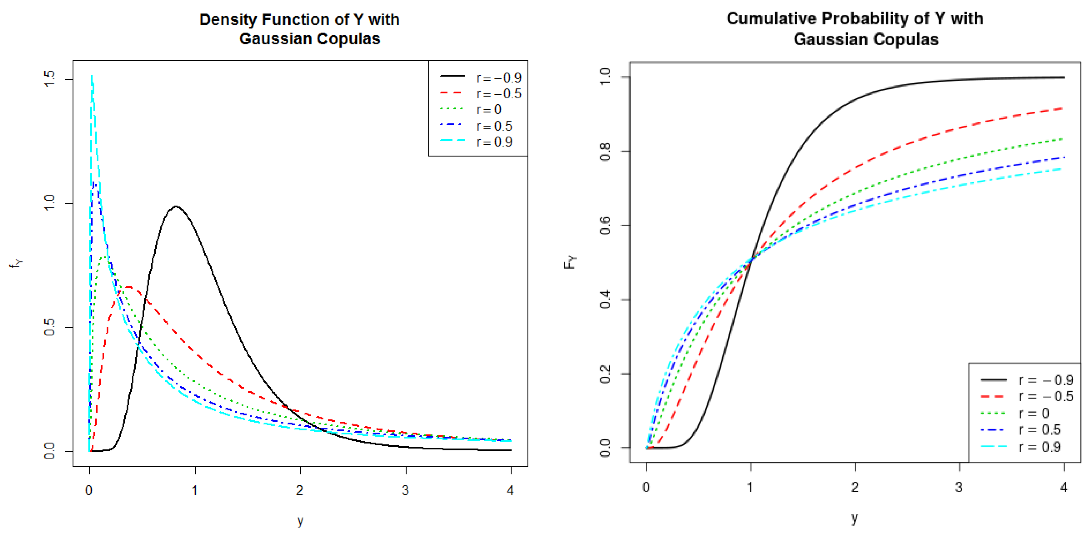
where ${\mathsf{\Phi }}^{-1}\left(x\right)$ is the inverse of standard normal CDF and r is Pearson correlation coefficient between $X_1$ and $X_2$ with $\left|r\right|<1$. Considering $r=-0.9,-0.5,0,0.5$, and $0.9$, we plot both PDFs and CDFs of Y in Figure 1 and display some descriptive statistics for $Y=X_1{X}_2$ in

Table 1. Descriptive Statistics for $Y=X_1{X}_2$ when $(X_1,X_2)$ follows Gaussian copulas.

r	$\mathit{\tau }\left({\mathit{C}}_{\mathit{r}}\right)$	Mean	Median	sd	Skewness	Kurtosis
$-0.9$	$-0.71$	1.11	1	0.52	1.51	7.30
$-0.5$	$-0.33$	1.65	1	2.16	5.84	85.43
0	0	2.72	1	6.77	14.27	466.41
0.5	0.33	4.48	1	18.21	23.23	1045.26
0.9	0.71	6.68	1	38.59	30.15	1585.27

, including the dependence measure Kendall $\tau$, mean, median, standard deviation (sd), skewness, and kurtosis. The special case of $r=0$ corresponds to the situation in which $X_1$ and $X_2$ are independent. As can be seen from the graph and table, for parameter $r\in [0,1]$ (positive correlation), PDFs of Y tends to be more right skewed than those from $r\in [-1,0)$ (negative correlation). When the parameter r varies from negative values to positive values, one can easily notice that the mean, sd, and kurtosis are all significantly increasing while the median is unchanged.

5.2. Student-t Copula

We turn to study the dependence structures of $X_1$ and $X_2$ through the following Student-t Copula $C_{r,\nu }(u,v)$:

$$C_{r,\nu }(u,v)={\displaystyle \frac{1}{2\pi \sqrt{1-r^2}}}{\int }_{-\infty }^{t_{\nu }^{-1}\left(u\right)}{\int }_{-\infty }^{t_{\nu }^{-1}\left(v\right)}{\left(1+{\displaystyle \frac{s^2-2rst+t^2}{v(1-r^2)}}\right)}^{(v+2)/2}dsdt,$$

and investigate the shape of the distribution for $Y=X_1{X}_2$ where $t_{\nu }^{-1}\left(x\right)$ is the inverse of Student CDF with $\nu$ degrees of freedom and r is the Pearson correlation coefficient between $X_1$ and $X_2$ with $\left|r\right|<1$ and the degree of freedom $\nu >2$.

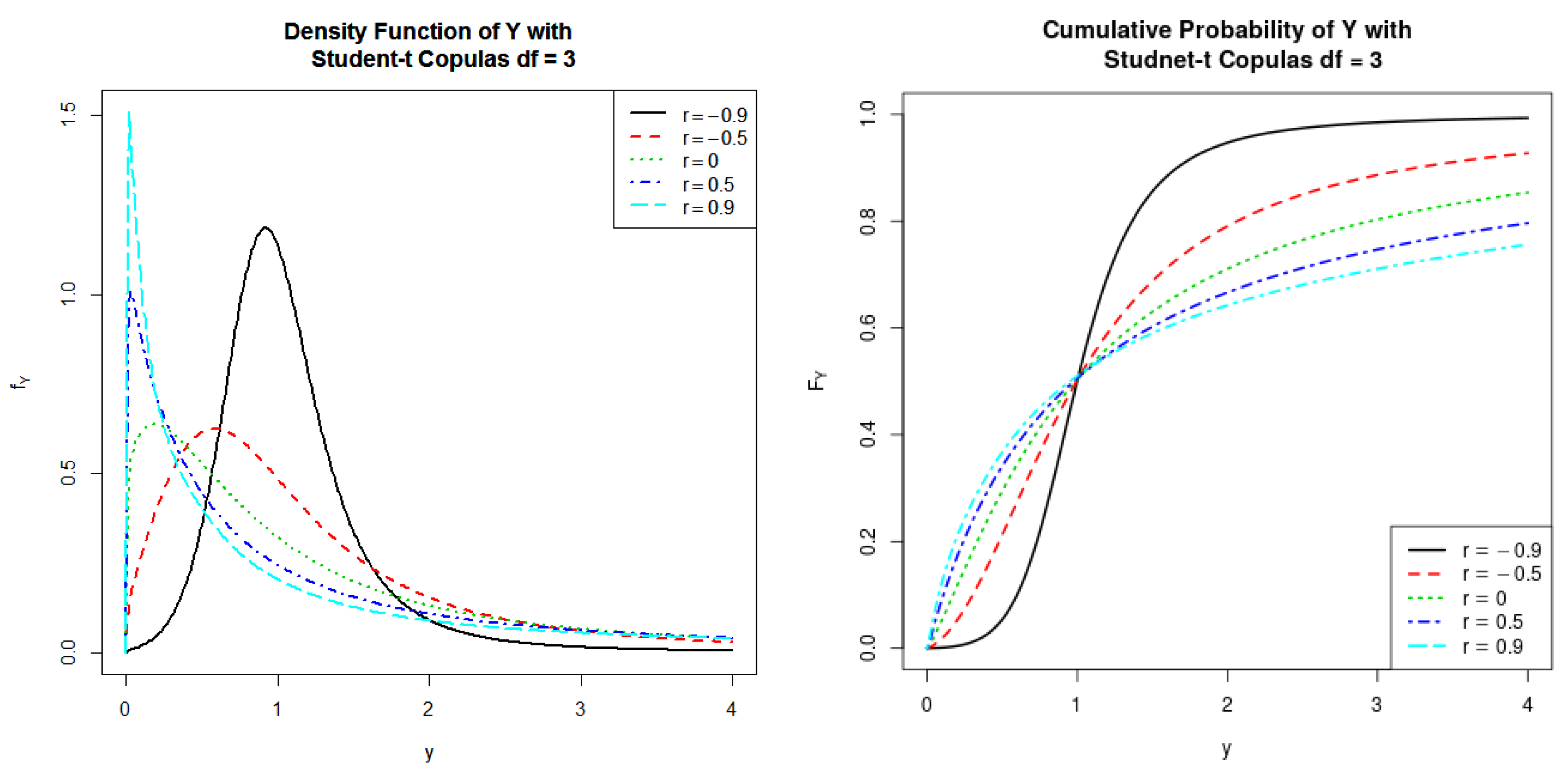
We illustrate our proposed approach by examining $r=-0.9,-0.5,0,0.5$, and $0.9$ with $\nu =3$. To do so, we first plot both PDFs and CDFs of Y in Figure 2 and exhibit some descriptive statistics for $Y=X_1{X}_2$ in

Table 2. Descriptive Statistics for $Y=X_1{X}_2$ when $(X_1,X_2)$ follows Student-t copulas, $\nu =3$.

r	$\mathit{\tau }\left({\mathit{C}}_{\mathit{r}}\right)$	Mean	Median	sd	Skewness	Kurtosis
$-0.9$	$-0.71$	1.13	1	1.42	3.62	2221.42
$-0.5$	$-0.33$	1.92	1	9.26	40.75	2562.20
0	0	3.30	1	20.44	37.01	2182.05
0.5	0.33	5.51	1	32.58	34.03	1903.21
0.9	0.71	6.89	1	44.09	32.31	1766.27

. Similar to the case of Gaussian copula, $r=0$ is for the case in which there is no linear correlation. We find that the more positive r is, the higher the mean and higher the variance of Y tend to be. However, different from the Gaussian case, Student t-copula can capture the tail dependence between $X_1$ and $X_2$ that yields larger kurtosis and larger skewness for Y than for the case of Gaussian copula.

5.3. Clayton Copula

We now investigate the dependence structures of $X_1$ and $X_2$ through the following Clayton Copula $C_{\theta }(u,v)$:

$$C_{\theta }(u,v)=\max {\left\{u^{-\theta }+v^{-\theta }-1,0\right\}}^{-{\displaystyle \frac{1}{\theta }}},\theta \in \left[-1;+\infty \right)\setminus 0,$$

(24)

and examine the shape of the distribution for Y.

We follow the common practice to use $\theta >0$ that leads to the following formula

$$C_{\theta }(u,v)={\left(u^{-\theta }+v^{-\theta }-1\right)}^{-{\displaystyle \frac{1}{\theta }}},\theta >0.$$

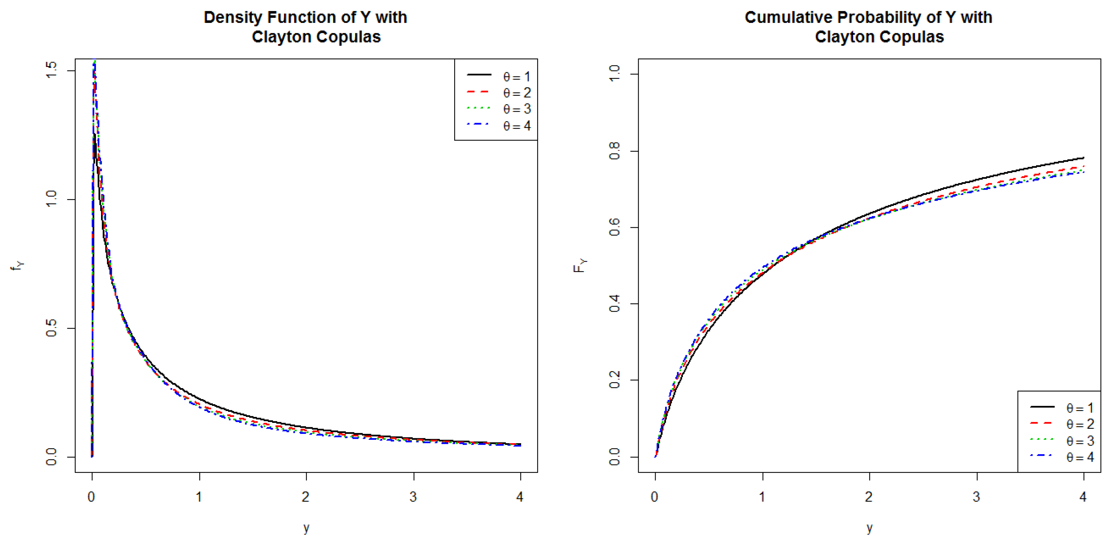
For $\theta =1,2,3$, and 4, we plot both PDFs and CDFs of Y in Figure 3. From the results in the figure, we confirm that Clayton copula can be used to model left tail dependence; that is, dependency at small values. We also find that, when parameter $\theta \to \infty$, it becomes more positive dependence and yields higher mean and higher standard deviation for Y but makes both the right skewness and the fatness of tail (kurtosis) smaller for Y (see

Table 3. Descriptive Statistics for $Y=X_1{X}_2$ when $(X_1,X_2)$ follows Clayton copulas.

$\mathit{\theta }$	$\mathit{\tau }\left({\mathit{C}}_{\mathit{\theta }}\right)$	Mean	Median	sd	Skewness	Kurtosis
1	0.33	3.53	1.12	8.93	13.12	403.90
2	0.5	4.01	1.13	10.43	12.81	389.76
3	0.60	4.34	1.11	11.55	12.65	379.99
4	0.67	4.59	1.08	12.41	12.36	359.40

).

5.4. Gumbel Copula

We turn to study the dependence structure of $X_1$ and $X_2$ through the following Gumbel Copula $C_{\theta }(u,v)$:

$$C_{\theta }(u,v)=\exp \left(-{\left[{(-\ln u)}^{\theta }+{(-\ln v)}^{\theta }\right]}^{{\displaystyle \frac{1}{\theta }}}\right),\theta >0,$$

and investigate the shape of the distributions for Y.

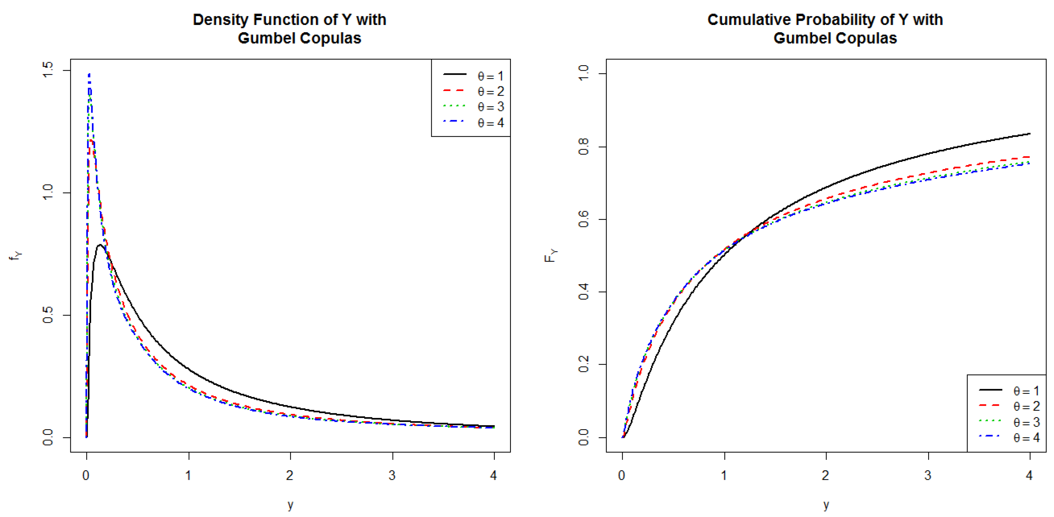
We plot both PDFs and CDFs of Y in Figure 4 for $\theta =1,2,3$, and 4. For Gumbel copula, $\theta =1$ is for the case in which $X_1$ and $X_2$ are independent. In contrast to Clayton, Gumbel copula is used to capture dependency at large values (right tail dependence). Hence, it makes Y to get bigger mean, higher variance, more right skewness, and heavier tail (kurtosis). However, in this case, the median is clearly smaller than that in the case of Clayton copula (see

Table 4. Descriptive Statistics for $Y=X_1{X}_2$ when $(X_1,X_2)$ follows Gumbel copulas.

$\mathit{\theta }$	$\mathit{\tau }\left({\mathit{C}}_{\mathit{\theta }}\right)$	Mean	Median	sd	Skewness	Kurtosis
1	0	2.72	1	6.78	14.41	477.10
2	0.5	6.47	0.95	41.52	32.34	1756.88
3	0.67	7.01	0.97	44.46	31.88	1719.80
4	0.75	7.19	0.98	44.83	31.66	1696.71

).

5.5. Frank Copula

We next examine the dependence structure of $X_1$ and $X_2$ through the following Frank Copula $C_{\theta }(u,v)$:

$$C_{\theta }(u,v)=-{\displaystyle \frac{1}{\theta }}\ln \left(1+{\displaystyle \frac{\left(e^{-\theta u}-1\right)\left(e^{-\theta v}-1\right)}{e^{-\theta }-1}}\right),\theta \in \mathbb{R}\setminus \left\{0\right\};$$

and study the shape of the distribution for Y.

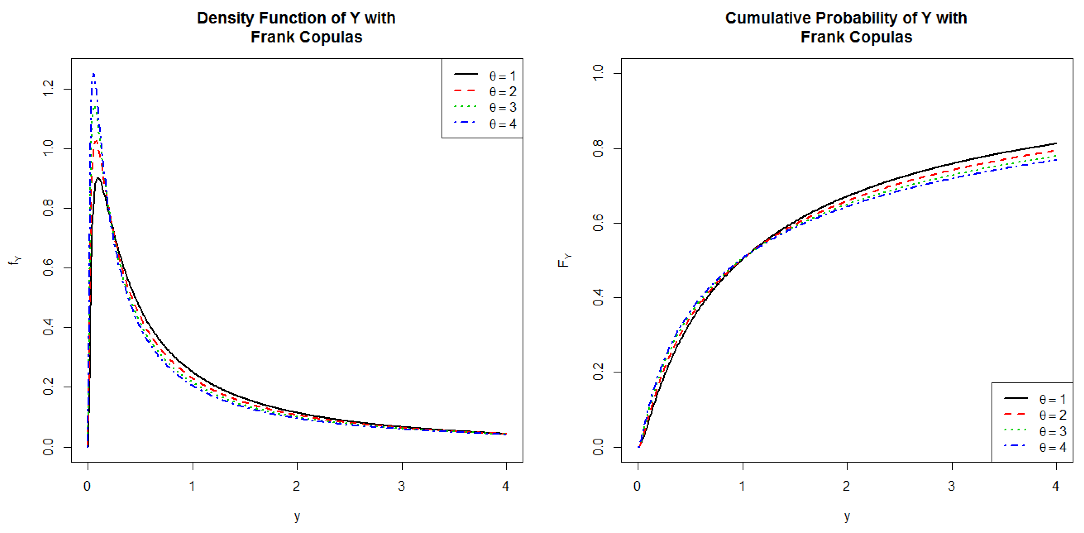
We plot both PDFs and CDFs of Y in Figure 5 for $\theta =1,2,3$, and 4 and display some descriptive statistics in

Table 5. Descriptive Statistics for $Y=X_1{X}_2$ when $(X_1,X_2)$ follows Frank copulas.

$\mathit{\theta }$	$\mathit{\tau }\left({\mathit{C}}_{\mathit{\theta }}\right)$	Mean	Median	sd	Skewness	Kurtosis
1	0.11	3.10	1	8.06	13.84	440.25
2	0.21	3.47	1	9.26	13.49	419.00
3	0.31	3.81	1	10.35	13.07	394.79
4	0.39	4.11	1	11.34	12.88	384.20

. For Frank copula, the parameter $\theta \to 0$ is for the case in which the two variables are independent. In addition, the structure becomes more monotonic when $\theta \to \infty$ and becomes counter monotonicity when $\theta \to -\infty$. Comparing with both Clayton and Gumbel, Frank copula cannot capture left or right tail dependence. It does not affect the median as in the case of both Gaussian and Student-t copulas. However, the mean and the standard deviation are higher and both skewness and fatness are smaller when the value of the parameter increases.

5.6. Joe Copula

Finally, we study the dependence structure of $X_1$ and $X_2$ through the following Joe Copula $C_{\theta }(u,v)$:

$$C_{\theta }(u,v)=1-{[{(1-u)}^{\theta }+{(1-v)}^{\theta }-{(1-u)}^{\theta }{(1-v)}^{\theta }]}^{1/\theta },\theta \in [1,\infty ),$$

and examine the shape of the distribution for Y.

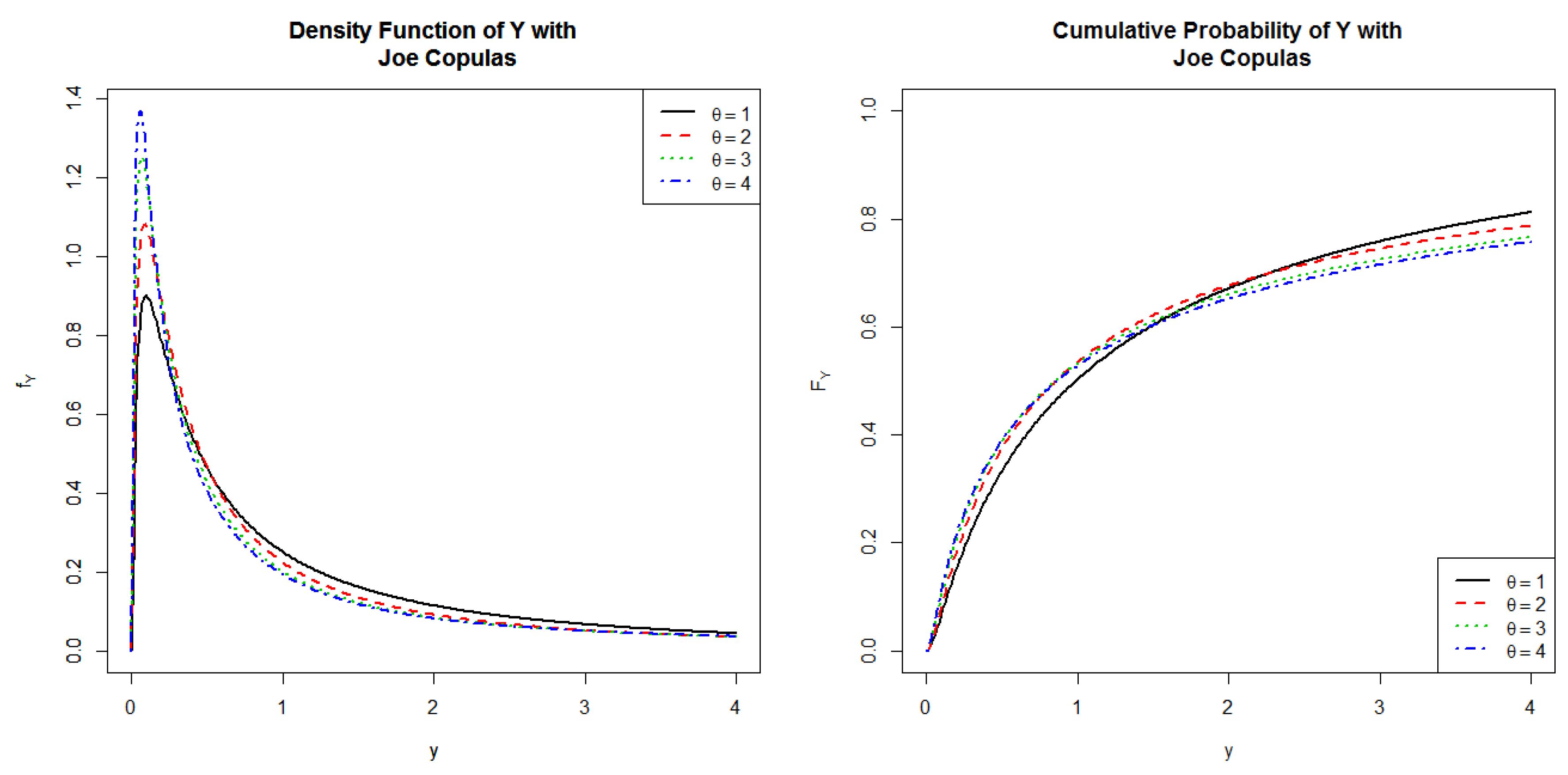
We plot both PDFs and CDFs of Y in Figure 6 for $\theta =1,2,3$, and 4 and display some descriptive statistics in

Table 6. Descriptive Statistics for $Y=X_1{X}_2$ when $(X_1,X_2)$ follows Joe copulas.

$\mathit{\theta }$	$\mathit{\tau }\left({\mathit{C}}_{\mathit{\theta }}\right)$	Mean	Median	sd	Skewness	Kurtosis
1	0	2.72	1.00	6.76	14.28	466.67
2	0.36	6.30	0.87	42.01	32.67	1789.96
3	0.52	6.91	0.88	44.31	31.65	1692.84
4	0.61	7.11	0.90	45.01	31.79	1720.81

. From the results in the figure and table, we find that the dependency captured by Joe Copula is similar to that captured by Gumbel Copula in the way that the variables are independence for $\theta =1$ and becomes more monotonic when $\theta \to \infty$. We also find that the variations of all other measures are changing in a similar manner.

5.7. Comparison of Copulas for the Same Measure of Dependence

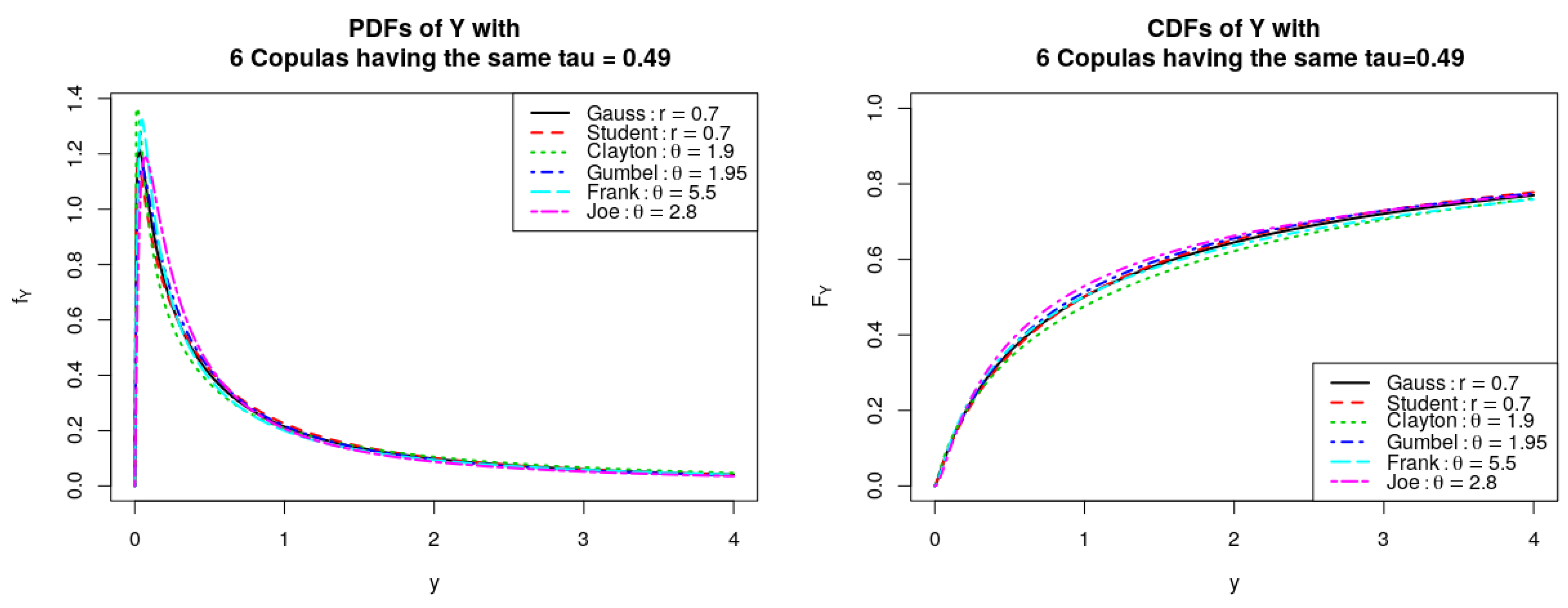
In this section, we investigate the effects of the six copulas families as discussed above on the shapes of different distributions for the random variable $Y:=X_1{X}_2$ when they have the same measure of dependence—the Kendall’s coefficient $\tau$. Here, the parameters are chosen to each copula to correspond to Kendall $\tau =0.49$. We exhibit the corresponding CDFs and PDFs of Y in Figure 7, estimate the mean, median, standard deviation, skewness, and kurtosis, and display the values in

Table 7. Descriptive Statistics for $Y=X_1{X}_2$ in which $(X_1,X_2)$ is modeled with six copulas having the same Kendall coefficient $\tau =0.49$.

Copulas	Parameters	$\mathit{\tau }\left(\mathit{C}\right)$	Mean	Median	sd	Skewness	Kurtosis
Gaussian	0.7	0.49	5.47	1.00	26.98	27.42	1375.98
Student-t	0.7, $\nu =3$	0.49	5.95	1.00	38.33	33.58	1876.99
Clayton	1.90	0.49	3.97	1.13	10.27	12.74	382.27
Gumbel	1.95	0.49	6.42	0.95	41.54	32.41	1764.93
Frank	5.5	0.49	4.47	1.00	12.58	12.59	362.17
Joe	2.8	0.49	6.84	0.87	44.67	32.37	1766.43

. As can be seen on the table and figure, Y attains the largest mean (6.84) and standard deviation (44.67) but the smallest median (0.87) when it follows Joe copula. In contrast, Clayton copula produces the smallest mean (0.39) and standard deviation (10.27) but attains the largest median (1.13). Using Student-t copula gets the largest skewness (33.58) and fatness (1876.99), followed by using Gumbel and Joe copulas. On the other hand, using Frank copula gets the lowest skewness (12.59) and the lowest fatness (362.17) for Y and Gaussian copula is ranked the fourth by mean, sd, skewness, and kurtosis.

6. Conclusions

Determining distributions of the functions of random variables is one of the most important problems in statistics and applied mathematics because it has wide range of applications in numerous areas including economics, finance, risk management, science, and many other areas, especially in modeling financial risk and derivatives. However, most studies only focus on structure for independent variables with some common distributions of the functions for the variables. There are few studies on determining distributions for statistical models involving dependence structure. Nonetheless, to the best of our knowledge, the problem of determining distribution function of product for two or more dependent random variables using copulas has not been studied. Thus, to bridge the gap in the literature, in this paper, we develop the theory to establish the formulas of both density and distribution functions for the product of two and more dependent and independent random variables via copulas to capture the structure among the variables.

Because the density and distribution of the product for dependent random variables are in terms of integrals, the forms of both density and distribution are very complicated, and, thus, it is very difficult, if not impossible, to obtain the exact forms of the density and distribution. To circumvent the problem, in this paper, we propose using Monte Carlo algorithm, graphical approach, and numerical analysis to efficiently compute their complicated integrals and examine the behaviors of both density and distribution and the changes of their shapes when parameters vary.

We illustrated our proposed approaches by using simulation and graphical approaches to study the behavior of the distribution for the product of two log-normal random variables on several different copulas, including Gaussian, Student-t, Clayton, Gumbel, Frank, and Joe Copulas. We found that different types of copulas have different impact on the behaviors of distributions. For example, since both Gaussian and Student-t copulas belong to elliptical family, their distributions of the product behave similarly. On the other hand, because Clayton, Gumbel, Frank, and Joe copulas belong to Archimedean family, their distributions of the product behave similarly but with impacts of different degrees. Furthermore, we found that there are some differences on location, variance, skewness, fatness of tail, and others when the values of the parameters vary.

In this paper, we derive formulas for both density and cumulative probability functions of the product of n random variables for $n\ge 2$. We also propose a Monte Carlo algorithm to compute both density and cumulative probability functions. The Monte Carlo algorithm we proposed enables academics and practitioners to obtain both density and cumulative probability functions easily. Furthermore, we drawn some useful information on the product of two lognormal-distributed random variables. Our results are the foundations of any further study that relies on the density and cumulative probability functions of the product of n random variables. We note that, although the theory we developed in our paper is not difficult to derive, as far as we know, our findings are new and there is no study obtaining similar results as our findings. Readers may read Cherubini et al. (2004); Nelsen (2007) for all related theories. Thus, the theory we developed in this paper is new, useful, and the contribution of our paper is important in the literature.

Our findings are useful to academics if studying the shapes and basic measures of both density and distributions of the product of dependent or independent random variables by using different copulas is their interest. Because the product of dependent or independent random variables by using different copulas are widely used in many empirical applications in economics, finance, and many other areas, our findings are useful to practitioners and policy makers in economics, finance, and many other areas if they need to study the shapes of both density and distribution functions for the product of dependent or independent random variables by using different copulas.

References

- Bohrnstedt, George W., and Arthur S. Goldberger. 1969. On the exact covariance of products of random variables. Journal of the American Statistical Association 64: 1439–42. [Google Scholar] [CrossRef]
- Cherubini, Umberto, Elisa Luciano, and Walter Vecchiato. 2004. Copula Methods in Finance. Hoboken: John Wiley & Sons. [Google Scholar]
- Cherubini, Umberto, Sabrina Mulinacci, and Silvia Romagnoli. 2011. A copula-based model of speculative price dynamics in discrete time. Journal of Multivariate Analysis 102: 1047–63. [Google Scholar] [CrossRef]
- Dettmann, Carl P., and Orestis Georgiou. 2009. Product of n independent uniform random variables. Statistics & Probability Letters 79: 2501–3. [Google Scholar]
- Donahue, James D. 1964. Products and Quotients of Random Variables and Their Applications. Technical Report. Fort Collins: MARTIN CO DENVER CO. [Google Scholar]
- Frey, Rüdiger, Alexander J. McNeil, and Mark Nyfeler. 2001. Copulas and credit models. Risk 10: 111–4. [Google Scholar]
- Galambos, Janos, and Italo Simonelli. 2004. Products of Random Variables: Applications to Problems of Physics and to Arithmetical Functions. Boca Raton: CRC Press. [Google Scholar]
- Garg, Mridula, Ajay Sharma, and Pratibha Manohar. 2016. The distribution of the product of two independent generalized trapezoidal random variables. Communications in Statistics-Theory and Methods 45: 6369–84. [Google Scholar] [CrossRef]
- Glen, Andrew G., Lawrence M. Leemis, and John H. Drew. 2004. Computing the distribution of the product of two continuous random variables. Computational Statistics & Data Analysis 44: 451–64. [Google Scholar]
- Joe, Harry. 1997. Multivariate Models and Multivariate Dependence Concepts. Boca Raton: Chapman and Hall/CRC. [Google Scholar]
- Lomnicki, Z. A. 1967. On the distribution of products of random variables. Journal of the Royal Statistical Society Series B (Methodological) 29: 513–24. [Google Scholar] [CrossRef]
- Ly, Sel, Hoang-Uyen Pham, and Radim Briš. 2016. On the distortion risk measure using copulas. In Applied Mathematics in Engineering and Reliability. Boca Raton: CRC Press, p. 309. [Google Scholar]
- Ly, Sel, Kim-Hung Pho, Sal Ly, and Wing-Keung Wong. 2019. Distribution of quotient of dependent and independent random variables using copulas. Journal of Risk and Financial Management. First revision. [Google Scholar]
- Maller, Ross A. 1981. A theorem on products of random variables, with application to regression. Australian Journal of Statistics 23: 177–85. [Google Scholar] [CrossRef]
- Nelsen, Roger B. 2007. An Introduction to Copulas. Berlin: Springer Science & Business Media. [Google Scholar]
- Salo, Jari, Hassan M. El-Sallabi, and Pertti Vainikainen. 2006. The distribution of the product of independent Rayleigh random variables. IEEE Transactions on Antennas and Propagation 54: 639–43. [Google Scholar] [CrossRef]
- Springer, Melvin Dale, and W. E. Thompson. 1966. The distribution of products of independent random variables. SIAM Journal on Applied Mathematics 14: 511–26. [Google Scholar] [CrossRef]
- Springer, Melvin Dale, and W. E. Thompson. 1970. The distribution of products of beta, gamma and Gaussian random variables. SIAM Journal on Applied Mathematics 18: 721–37. [Google Scholar] [CrossRef]
- Springer, Melvin Dale. 1979. The Algebra of Random Variables, 1st ed. Hoboken: Wiley. [Google Scholar]
- Tang, Jiechen, Songsak Sriboonchitta, Vicente Ramos, and Wing-Keung Wong. 2014. Modelling dependence between tourism demand and exchange rate using copula-based GARCH model. Current Issues in Method and Practice 19: 1–19. [Google Scholar] [CrossRef]
- Tran, Duy-Hien, Hoang-Uyen Pham, Sel Ly, and Trung Vo-Duy. 2015. A new measure of monotone dependence by using Sobolev norms for copula. In International Symposium on Integrated Uncertainty in Knowledge Modelling and Decision Making. Belin: Springer, pp. 126–37. [Google Scholar]
- Tran, Duy-Hien, Hoang-Uyen Pham, Sel Ly, and Trung Vo-Duy. 2017. Extraction dependence structure of distorted copulas via a measure of dependence. Annals of Operations Research 256: 221–36. [Google Scholar] [CrossRef]
- Yang, Yang, and Yuebao Wang. 2013. Tail behavior of the product of two dependent random variables with applications to risk theory. Extremes 16: 55–74. [Google Scholar] [CrossRef]
Figure 1.
PDFs and CDFs of the product of two log-normal distributed random variables having Gaussian Copulas.
Figure 2.
PDFs and CDFs of the product of two log-normal distributed random variables having Student t-Copulas .
Figure 3.
PDFs and CDFs of the product of two log-normal distributed random variables having Clayton Copulas.
Figure 4.
PDFs and CDFs of the product of two log-normal distributed random variables having Gumbel Copulas.
Figure 5.
PDFs and CDFs of the product of two log-normal distributed random variables having Frank Copulas.
Figure 6.
PDFs and CDFs of the product of two log-normal distributed random variables having Joe Copulas.
Figure 7.
PDFs and CDFs of the product of two log-normal distributed random variables with six copulas having the same Kendall coefficient.