1. Introduction
A reverse mortgage allows the owner of a home property to make a loan based on the value of the property while keeping the right to stay in the property for life. If the homeowner dies or moves out, the sale proceeds of the property are used to pay back the loan as well as the accumulated interest. In Australia, each product usually has a no-negative-equity guarantee such that the total final payment is no more than the sale value of the mortgaged property. Seniors and retirees can use a reverse mortgage to unlock their home equity and obtain extra funding to pay for their living expenses and other needs. Under the ageing population and the common problem of being asset-rich-cash-poor
1, reverse mortgages represent a financially feasible solution for millions of households. This market has been growing quite steadily in Australia
2.
Providers of reverse mortgages encounter a wide range of market, insurance and business risks. It is of utmost importance to assess these different risks adequately in pricing and reserving. Generally speaking, the main ones are house price risk, interest rate risk, longevity risk and other types of business risks. First, if the homeowner lives longer than anticipated, the exposure and thus the chance of the property value dropping below the accumulated loan balance would be increased. Second, the house price and the interest rate fluctuate over time and are subject to economic cycles, leading to uncertainty in the financial outcomes. Moreover, there are various types of common business issues such as fraud, legal risk and operational risk.
In the literature of pricing reverse mortgages, many of the authors assumed a fixed interest rate and allowed for either longevity risk or house price risk or both (e.g.,
Debón et al. 2013;
Ji et al. 2012;
Kogure et al. 2014). A few took all of the house price risk, interest rate risk and longevity risk into account but used different pricing methods for these three risks separately (e.g.,
Wang et al. 2008;
Lee et al. 2012). In this article, we suggest a Bayesian approach to include all the three risk components in a more consistent manner. Particularly, we adopt the maximum entropy approach (
Kogure and Kurachi 2010;
J. S.-H. Li 2010) in risk-neutralisation, which has some potential advantages over the other pricing methods such as the Esscher transform and Wang transform. It is more flexible in terms of being able to incorporate more than one market price, allowing the use of different simulation methods, and pricing multiple risk factors within the same framework. Moreover, Bayesian modelling offers a number of desirable features. One can estimate the mortality structure and the time series process more coherently in a single step, rather than the usual two separate steps in most of the previous mortality projection work. It is relatively straightforward to deal with missing values, which can be an important issue when the market is not fully developed and only limited data are available. Other reference information may also be incorporated into the priors to assist in parameter estimation. Finally, both process error and parameter error (uncertainty in estimating parameters), and possibly model error (uncertainty in choosing between models), can readily be allowed for in the Bayesian modelling process.
The remaining parts are presented as follows.
Section 2 sets forth the concept of applying the principle of maximum entropy in pricing reverse mortgages.
Section 3 introduces the Bayesian models we adopt for modelling house price risk, interest rate risk and longevity risk.
Section 4 discusses the numerical results of a hypothetical example based on Australian data and provides the analysis.
Section 5 gives the concluding remarks.
2. Pricing Mechanism
Let
be the random value of a risk factor at time
,
be its real-world probability density function (pdf),
be the random payoff of the
ith security at time
,
be the time-0 market price of that security and
be the risk-free interest rate. Under the principle of maximum entropy, the risk-neutral pdf
is obtained by minimising the Kullback–Leibler information criterion
, subject to the constraints
and
for
. This pricing method has several advantages. Firstly, any number
of market prices can be embedded into the constraints in principle. This property is suitable for the currently developing and illiquid life market. Secondly, different simulation and bootstrapping methods (e.g.,
J. Li 2014a) can readily be implemented under this method. It allows one to avoid complex derivations and facilitates implementation in practice. Thirdly, this method can be applied to multiple risk factors simultaneously. This treatment is arguably more consistent or coherent than the way of arbitrarily applying different risk-neutral measures to different risk factors, which is usually seen in the literature. Finally, there are both theoretical arguments and empirical evidence supporting the use of this pricing method. For instance, the maximum entropy principle is closely related to the expected utility hypothesis, and this measure can produce prices similar to Black–Scholes ones in a simulated environment based on the Black–Scholes model settings (e.g.,
J. S.-H. Li 2010).
In the next two sections, we use Bayesian modelling to generate
random scenarios with equal real-world probability
for
. Accordingly, we utilise the discrete form of the maximum entropy principle, in which the Kullback–Leibler information criterion becomes
and the constraints are
and
. The term
represents the risk-neutral probability and
is the
jth simulated payoff of the
ith security at time
. The Lagrange expression is stated as:
in which
and
are the Lagrange multipliers. To find the risk-neutral probabilities
which minimise the Kullback–Leibler information criterion, all the partial derivatives of the Lagrange expression are first set to zero:
The last two equations are just the two constraints, while the first one can be expressed as:
Since
, the following can be deduced:
The Lagrange multipliers
and so the risk-neutral probabilities
can then be obtained by incorporating Equation (1) into the market price constraints
and using numerical optimisation to solve the resulting equations
3.
The derivation above is based on one risk factor and can readily be extended to multiple risk factors. For instance, the following equation can be used when all of the house price risk, interest rate risk and longevity risk are integrated into pricing a reverse mortgage:
where
is the simulated time-0 present value of the
ith security in the
jth scenario. The value of each security is a function of one or two or all of the three risk factors. Note that the underlying discount rate can be treated as stochastic in this more generalised setting.
3. Bayesian Modelling
Consider a person aged
who has purchased a reverse mortgage at time 0. Let
be the outstanding loan balance and
be the mortgaged property’s market value at time
. Suppose the loan interest rate is constant at
p.a. and so
. When the borrower dies between time
and time
, the loan is terminated and the lender receives a lump sum of
at time
4. In effect,
refers to the potential payoff to the homeowner from the no-negative-equity guarantee, which can be viewed as a put option written on the house price with a moving strike price. For a large portfolio of borrowers
5 from the same birth cohort with homogenous house price growth experience and mortality improvement, define
as the future percentage of this group who die between time
and time
. The lender then receives
at
on average per borrower. Denote
as the risk-free rate per annum covering time 0 to time
. The time-0 expected present value of the reverse mortgage per capita is
under the risk-neutral measure. The reverse mortgage is financially viable for the lender if this expected present value is larger than the initial loan size
. Note that there are three stochastic variables in this formula:
(interest rate risk),
(house price risk) and
(longevity risk), which require proper modelling to allow for their uncertainties. It is assumed that longevity risk and market risks are real-world independent.
We set
, in which
is the mortality rate that a life aged
at time
dies during the next year. Assuming the force of mortality
remains unchanged within every age–time cell and it is equal to the central death rate
, it can be deduced that
. We use the well-known
Lee and Carter (
1992) model
, where
describes the overall age schedule and
measures the age-sensitivity of the log central death rate to the mortality index
6. We assume the number of deaths
with
as the central exposed to risk, and the random walk with drift
for the mortality index, in which
is the drift and
. Under the Bayesian framework, following
Kogure et al. (
2009) and
J. Li (
2014b), we set the priors
,
,
and
7. The major step is to obtain the posterior distribution of the unknown quantities and parameters given the dataset, using
. However, the derivation of an explicit solution of the posterior density is intractable for the models being used here. Therefore, we utilise the Markov chain Monte Carlo (MCMC) method to simulate random samples based on a Markov chain which has its stationary distribution equivalent to the required posterior distribution. These random samples are then put into Equations (1) or (2) to compute the risk-neutral probabilities.
To cope with the autocorrelations and cross-correlations found in the house price growth rates
8 and interest rates, we adopt the vector autoregressive process, VAR(
):
where
,
’s are the autoregressive coefficients and
are bivariate normal with zero mean. As stated in
Rosenberg and Young (
1999), autoregressive processes are more straightforward to implement in a Bayesian setting compared to moving-average processes. If the order
of the autoregressive terms is high enough, the modelling results would be similar to a given autoregressive moving-average process. We set the prior of
’s as multivariate normal with zero mean, and the prior of the inverse covariance matrix of
distributed as Wishart
9.
In the MCMC simulation process, we discard the starting 5000 iterations in order to eliminate the impact of the initial values and collect 1000 sample paths afterwards. As shown in the
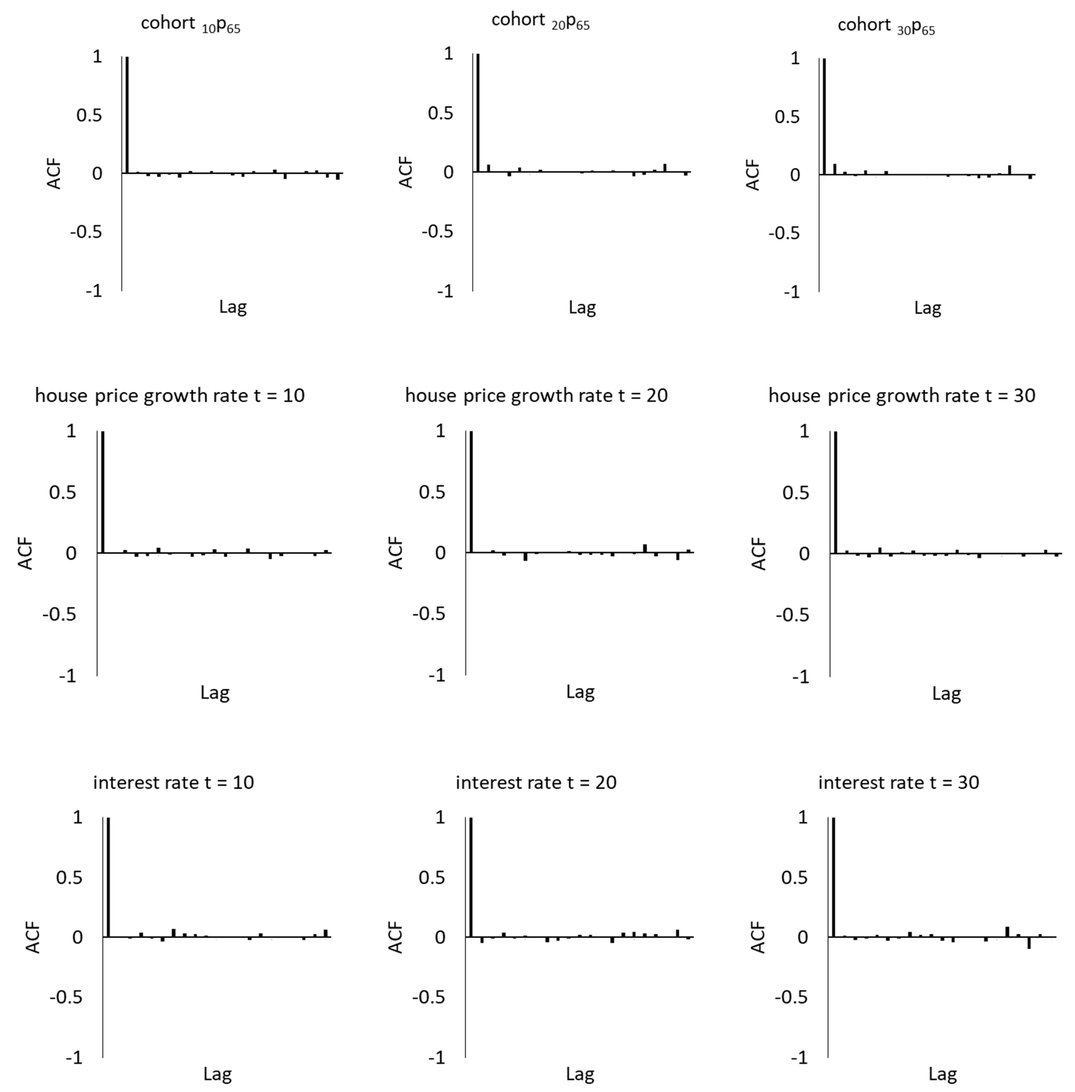
Appendix A, the resulting autocorrelations between successive MCMC samples of each variable are minimal, which suggest that the extent of convergence is adequate in our computations. We apply the Bayesian software WinBUGS (
Spiegelhalter et al. 2003) to perform the MCMC simulation via Gibbs sampling. The fundamental idea is to sequentially generate samples from the distribution of each variable conditional on all the other variables.
J. Li (
2014b) provided some examples of writing WinBUGS codes for projection and simulation of future death rates.
4. Analysis of Modelling Results
We obtain Australian male mortality data from the Human Mortality Database (
HMD 2018) for a period of 40 years from 1975 to 2014 and an age range of 65 to 99.
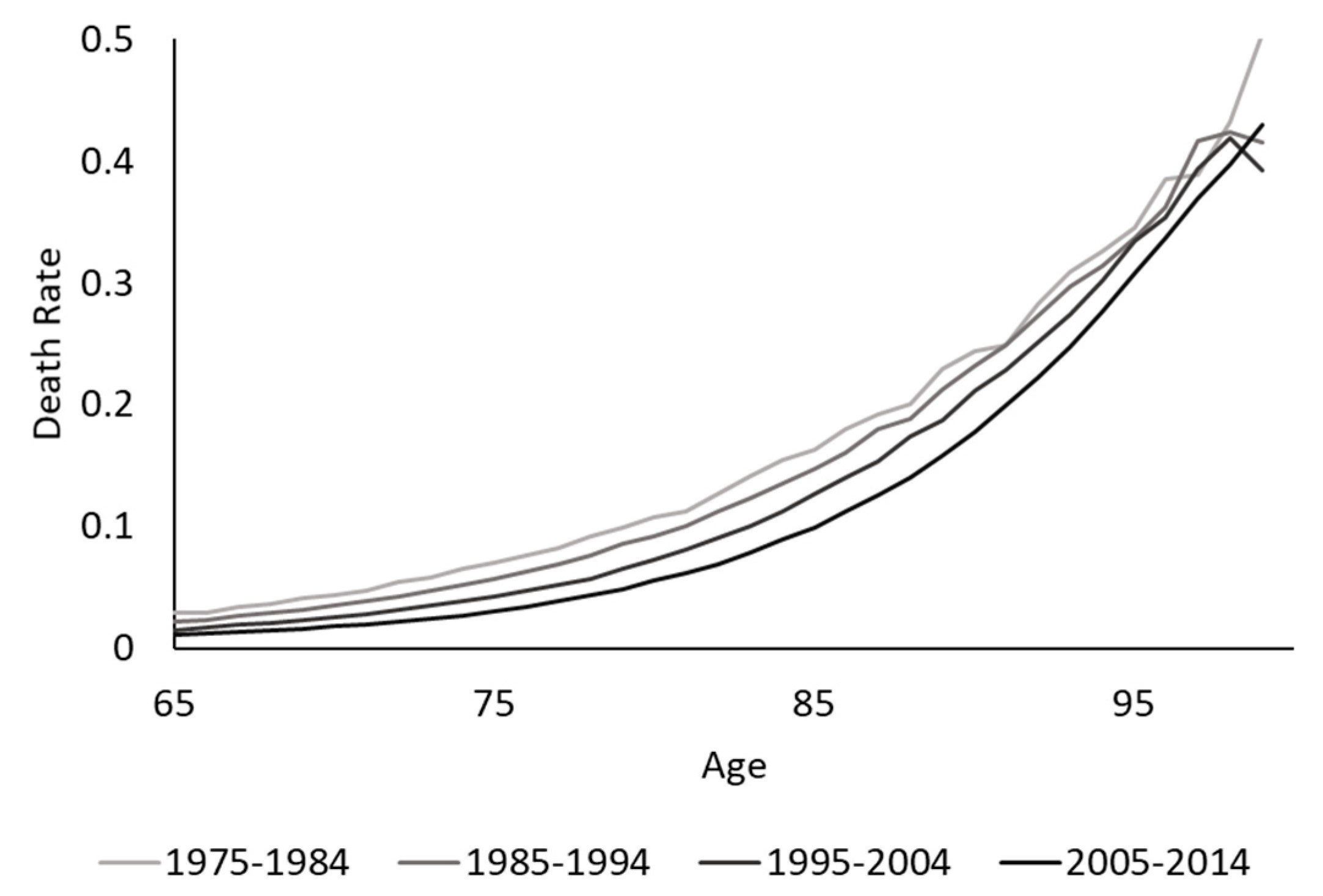
Figure 1 exhibits the central death rates across age for each decade. It can be seen that generally there has been a continual mortality improvement over time. The extent appears to be more significant at ages 80 and above in the most recent period.
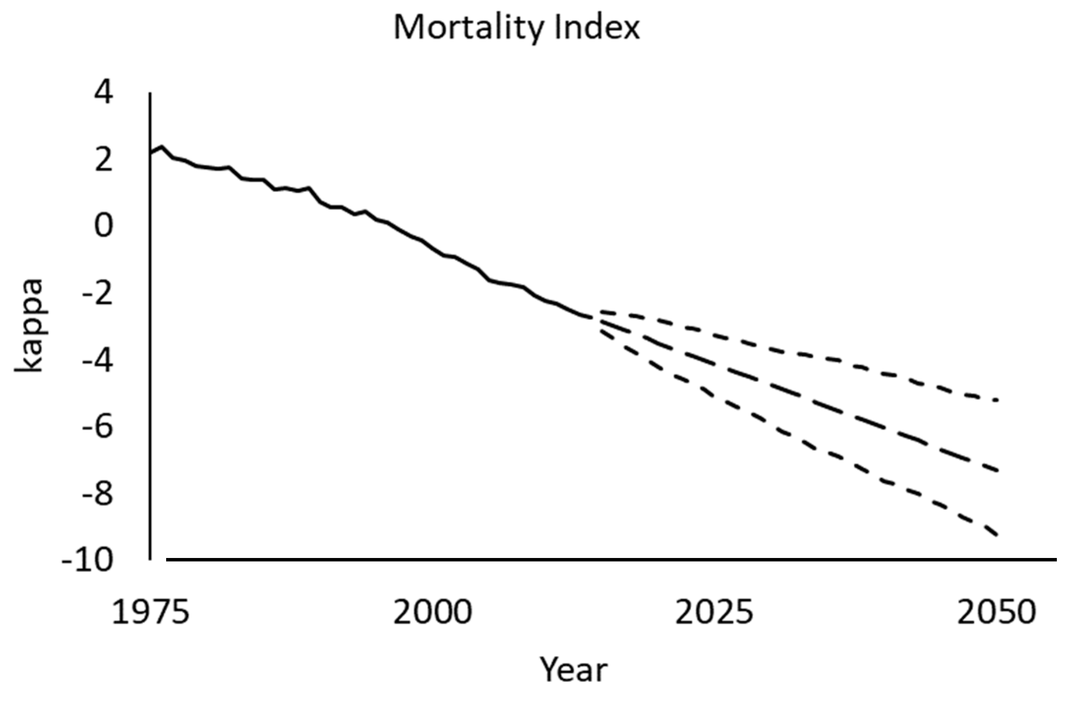
Figure 2 presents the estimated Lee–Carter mortality index, which is decreasing mostly linearly across time, and its projected central values (sample means) and the corresponding 95% prediction intervals from the MCMC simulation.
Figure 3 displays the simulated density functions of the future survival probabilities from age 65 (at time 0) to ages 75, 85 and 95.
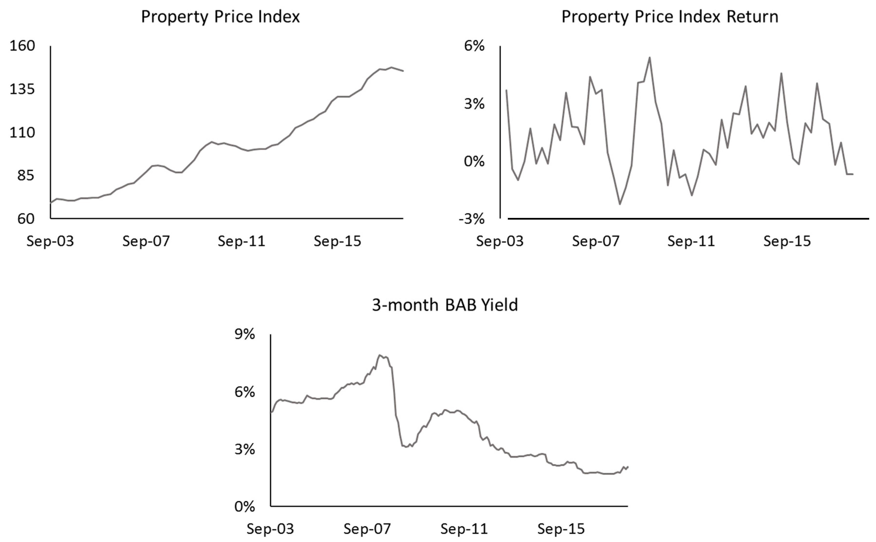
We collect the quarterly residential property price index values (calculated as a weighted average of eight capital cities) from the Australian Bureau of Statistics (ABS) for the period 2003 to 2018. We also obtain the 3-month bank accepted bills yields from the Reserve Bank of Australia (RBA) for the same period. Note that the property price index (a price-based index) is taken as a proxy, as each property is unique by nature itself and is infrequently traded.
Figure 4 shows that the overall property market in Australia has experienced significant growth over the past sixteen years. Despite this major trend, the house prices do not simply increase linearly but move in some forms of cycles. The quarterly growth rates during the period actually range widely from −2.2% to 5.4%. The figure also demonstrates the cyclical interest rate movements for the period and the broad level has decreased from above 5% p.a. to around 2% p.a. of late.
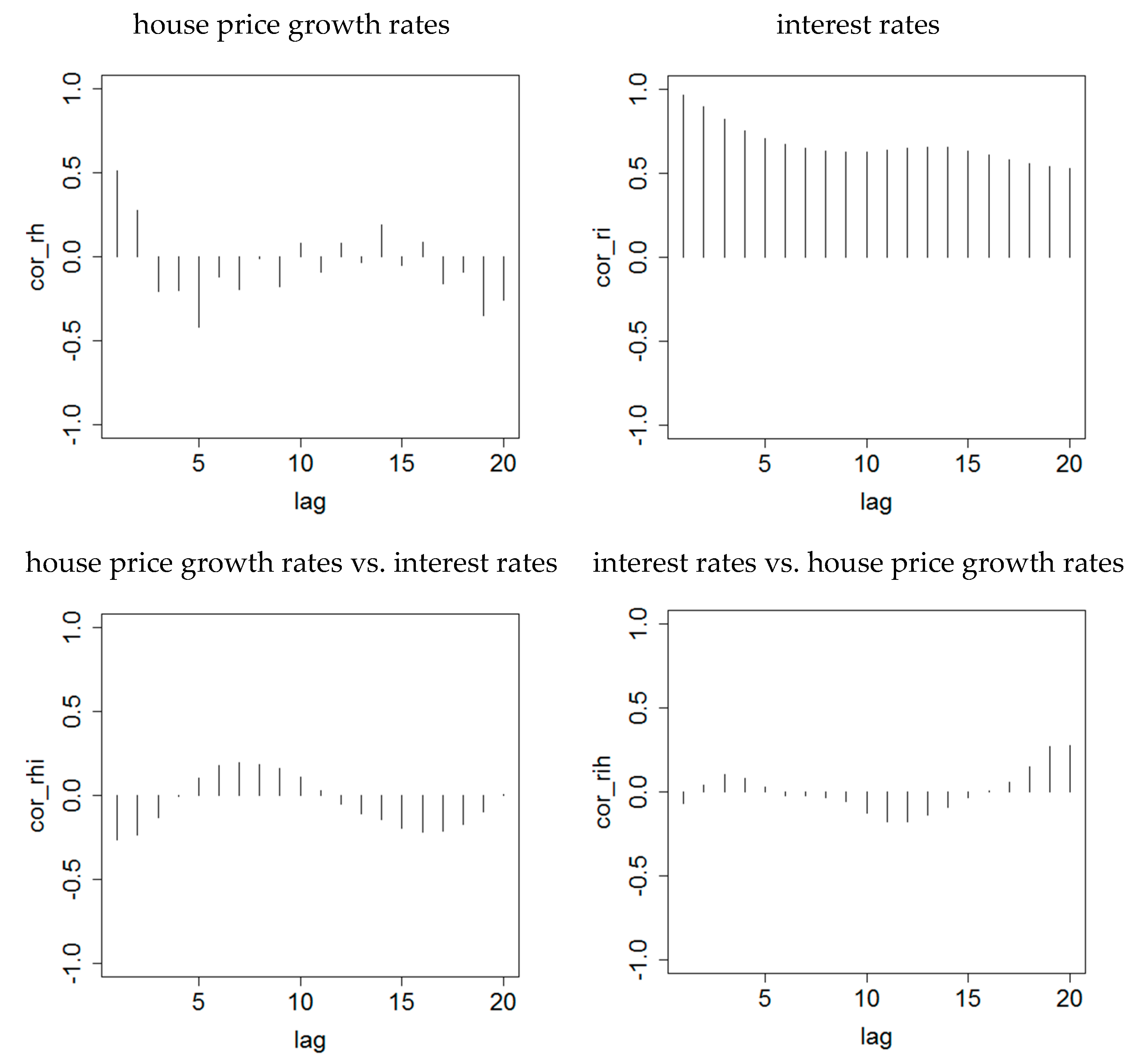
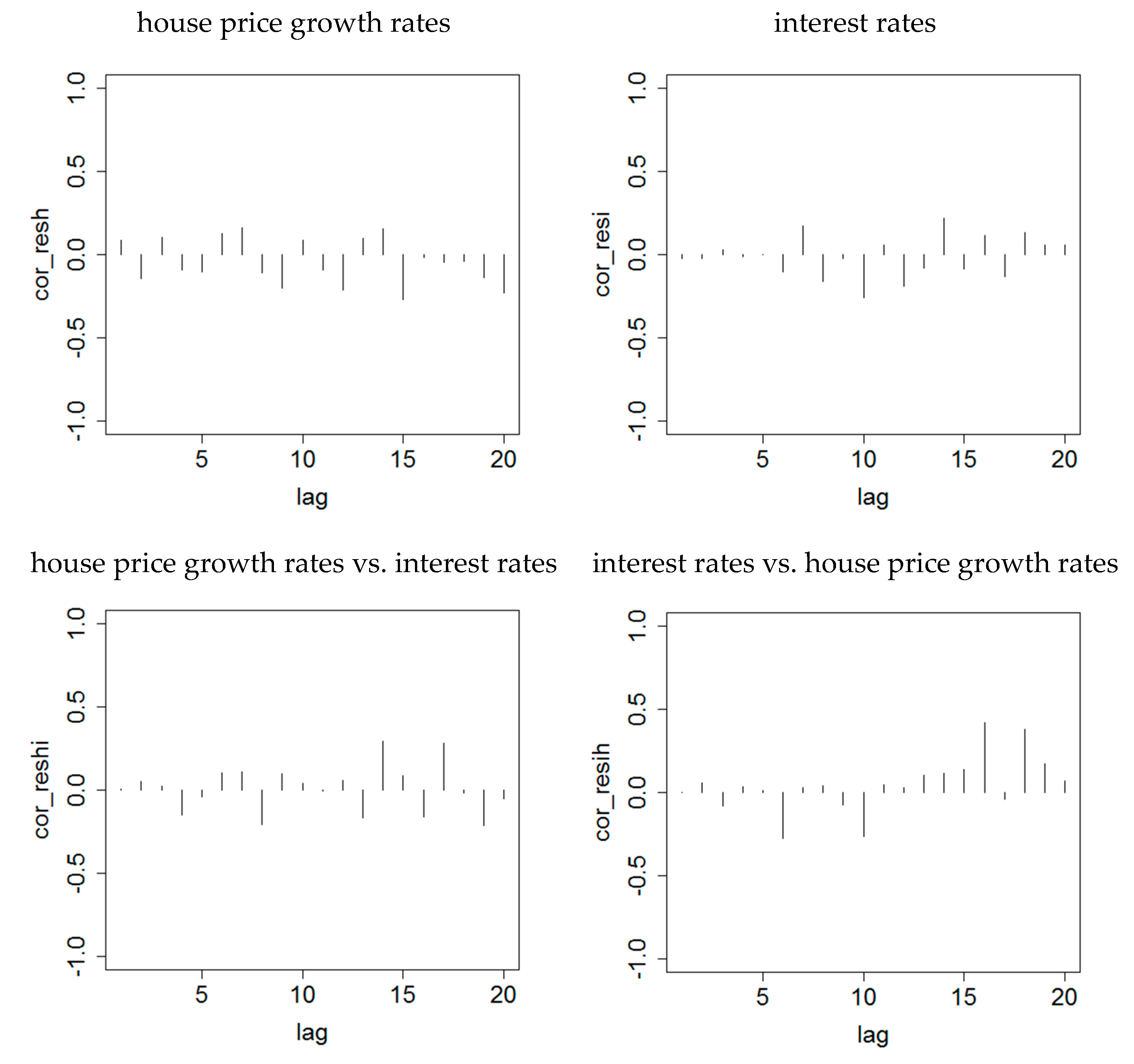
Figure 5 illustrates that there are significant sample autocorrelations and cross-correlations in between the time series of the house price growth rates and interest rates. A bivariate autoregressive process can be adopted to capture these time-dependent patterns. After examining the sample partial autocorrelation matrices and the sample cross-correlation matrices, we notice that a VAR(5) process (i.e., a maximum lag of five quarters) appears to fit the data reasonably well and the corresponding residuals do not have significant time-varying patterns in general, as shown in
Figure 6. The sample autocorrelations of the squared residuals are also found to be insignificant and so a GARCH-type model for conditional heteroscedasticity is not required here.
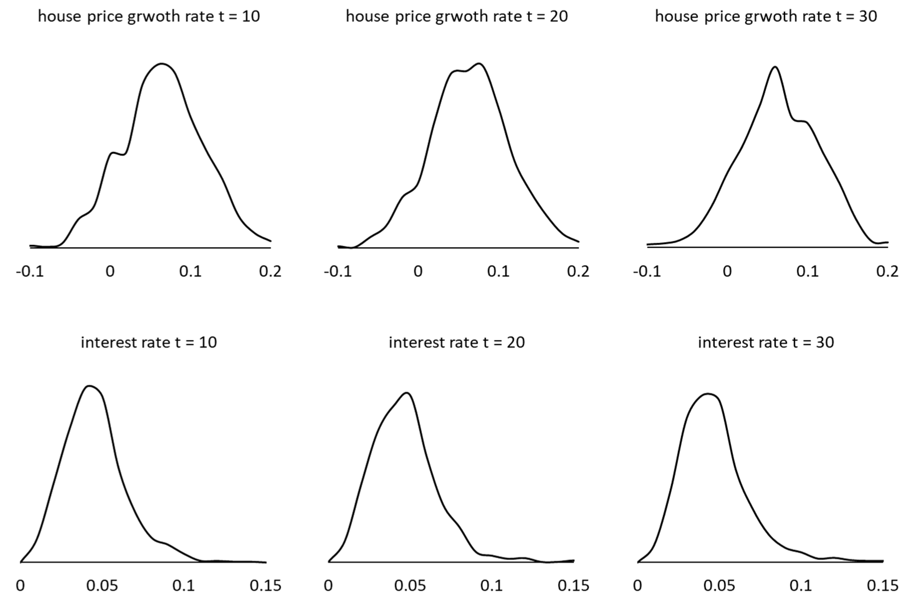
Figure 7 plots the simulated density functions of the future quarterly house price growth rates and interest rates after 10, 20 and 30 years.
Since the Australian annuity market is very thin, we use the mortality investigation reports published by the Institute of Actuaries of Australia
10 and the underlying improvement rates to deduce the annuity market price. We also take the ABS property price index as the house market price, and collect the latest Australian government bond price in the market. These market prices are substituted into the constraints as noted in
Section 2.
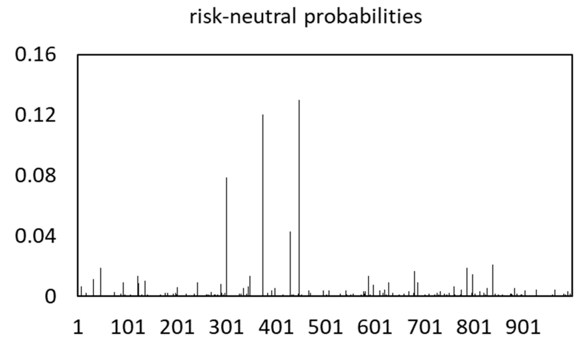
Figure 8 exhibits the resulting risk-neutral probabilities.
Suppose the valuation date (
t = 0) is as at the start of 2019 and
P0 = 550,000
11. We consider an individual aged 65 or 75 entering into a reverse mortgage contract with a loan-to-value (LTV) ratio of 10%, 20%, …, or 100%, i.e.,
L0 = 55,000, 110,000, …, or 550,000, and
l = 1%, 2%, …, or 10% p.a
12. These are a total of 200 cases in which we examine the calculated market prices of the reverse mortgage based on the different terms being offered.
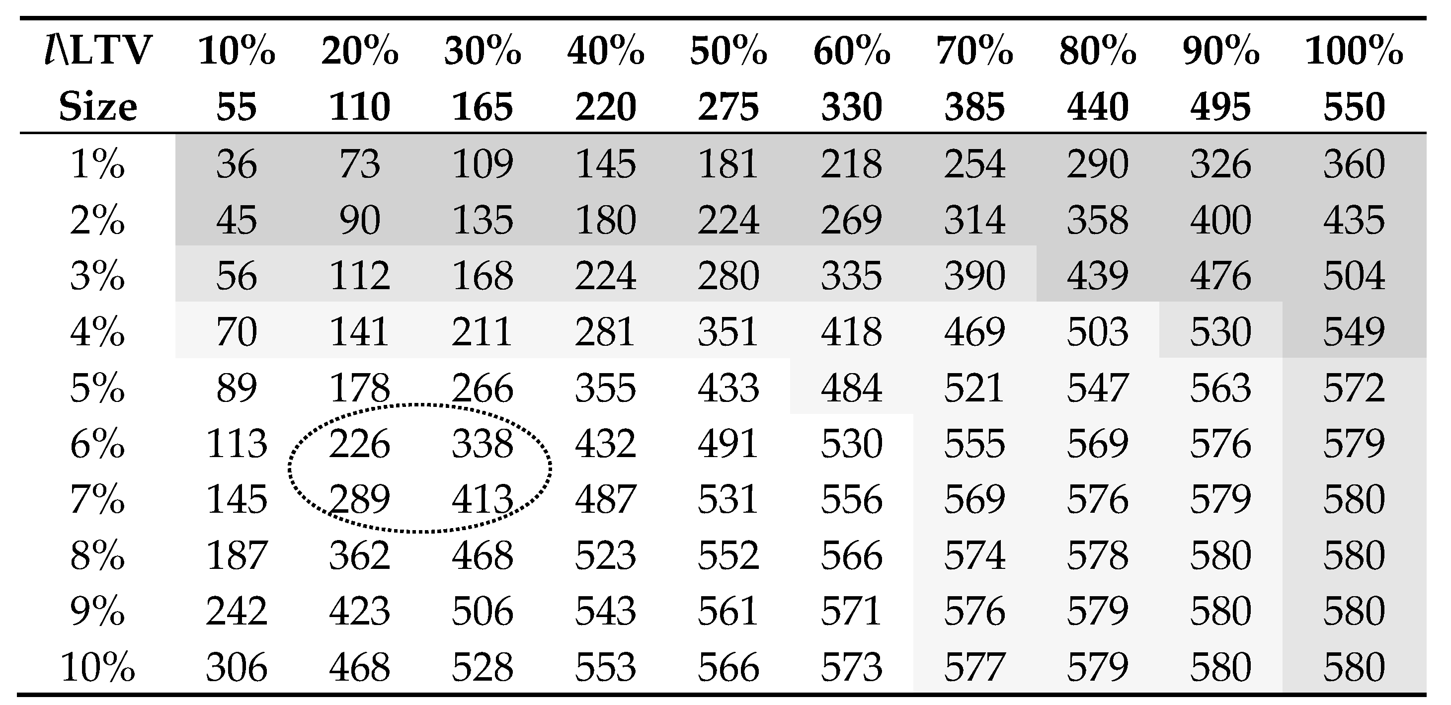
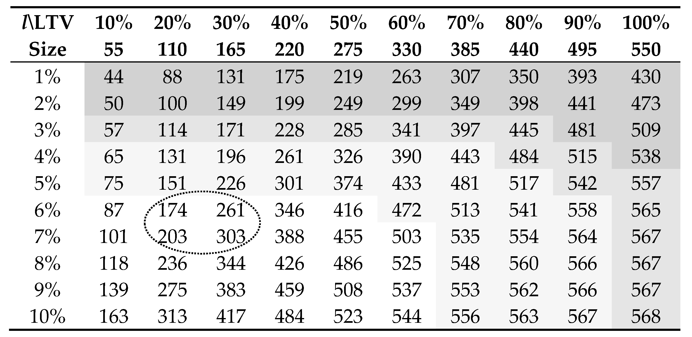
Table 1 and
Table 2 give the (risk-neutral) expected present values of the reverse mortgage under various loan interest rates and LTV ratios. When the loan interest rate is 1% or 2% p.a., the initial loan size is larger than the expected present value, and the reverse mortgage is then financially infeasible for the lender. As the loan interest rate rises, the reverse mortgage value increases and the contract becomes more feasible for the lender. But this effect is lesser if the LTV ratio is higher, because under the no-negative-equity guarantee, the embedded put option is worth more when there is a higher chance for the market value of the mortgaged property to be lower than the accumulated loan balance. In the current market, the loan interest rate is above 6% p.a. for reverse mortgages (see
Table 3), which is 1% to 2% higher than for a standard home loan, and the LTV ratio is around 20% (30%) for a borrower aged 65 (75). The figures in
Table 1 and
Table 2 pinpoint that the reverse mortgage products presently offered are financially viable from the providers’ perspective.
To further differentiate the outcomes, we also examine the percentage differences between the expected present value and the initial loan size in each case. Ignoring expenses (e.g., commissions, distribution costs), in
Table 1 and
Table 2, those cases incurring a loss are shaded as dark grey; the offers that generate a less than 10% profit are noted as medium grey; those giving 10% to 50% of profit are highlighted as light grey; and all the other cases with more than 50% gain are not shaded. It seems that the current providers are actually overly conservative in designing their products (the range of which is circled) and the existing market offers tend to be too expensive. There appears to be some room for Australian banks and insurers to provide more attractive products by increasing the LTV ratio, decreasing the loan interest rate or delivering more flexible solutions. As noted in Australian Securities and Investments Commission (
ASIC 2018), however, the current market is highly concentrated with the largest four lenders accounting for 92% of new approved loans during 2013 to 2017. The lenders imposed limits on the maximum LTV ratio which were lower than the levels prescribed in the enhanced consumer protections. There may also be a barrier for lenders to enter the market such as the capital requirement and the difficulty accessing wholesale funding after the global financial crisis. Besides improving the protection for customers’ interests, the government can actually consider giving more incentives for the industry to supply reverse mortgage products (e.g., the US Home Equity Conversion Mortgage program managed by the Department of Housing and Urban Development). More education and promotion can also be used to increase the public awareness of these products in an ageing society.
5. Concluding Remarks
Our proposed Bayesian multivariate risk-neutral pricing method has been shown to be very flexible in dealing with multiple risks and setting market price constraints. It gives a more coherent treatment of the various steps and components, compared to the other earlier approaches on pricing reverse mortgages. The results of our case study further suggest that a reverse mortgage provider in Australia can operate in a sustainable manner, under the current financial environment and the model settings and assumptions.
There are a number of areas which require future research. While we have focused on a plain vanilla type of reverse mortgage, there are other features that are worth studying such as joint lives, multiple decrements and a variety of other product designs (e.g., income payments, variable loan interest rate, capital protection and long-term care). Relevant prior information can be put into the modelling process and the resulting impact can be investigated. One can also replace the Lee–Carter model and the VAR process with other models and compare the corresponding results. Furthermore, model uncertainty can further be integrated by setting prior probabilities on a few pre-selected model choices and then deriving their posterior distributions.
