1. Introduction
Variable annuities (VAs) are equity-linked accumulation products that provide the policyholder tax-deferred growth on investments. They are often used as retirement savings vehicles and can provide protection against downside equity market risk. This protection stems from various riders that provide guaranteed minimum values of various contract elements; they are generically referred to as GMxB. A few common examples include the guaranteed minimum death benefit (GMDB), guaranteed minimum accumulation benefit (GMAB), guaranteed minimum withdrawal benefit (GMWB), guaranteed minimum maturity benefit (GMMB), and guaranteed minimum income benefit (GMIB). VAs saw dramatic increases in popularity after these guarantees were introduced in the 1990s and early 2000s in the US and many markets worldwide, including Canada, the UK, Japan, and in some European markets (
Bauer et al. 2008;
Ledlie et al. 2008), in part because of the protection against market downturns they provide. More recently, this popularity has fluctuated and has been trending downward: In 2008, VA sales in the US were estimated to be
$156 billion, whereas by 2017, this figure had shrunk to
$96 billion (
LIMRA 2018). This product line nonetheless represents a very significant block of business for insurers, with industry-wide net assets in the US for VA products totaling approximately
$2 trillion at the end of 2017 (
Insured Retirement Institute 2018).
Two of the fundamental actuarial tasks associated with these VA products are (1) pricing the guarantee, and (2) provisioning (reserving) for the guarantee, which may involve determining how much capital to hold, or devising a method for hedging the guarantee. As VA guarantees can often be viewed as granting a financial option to the policyholder (
Hardy 2003), it is perhaps not surprising that ideas from option pricing and hedging have often been utilized in the pricing and hedging of these types of guarantees. Two of the earlier examples of this include
Brennan and Schwartz (
1976), who considered the pricing of a variable life insurance product with a guaranteed minimum benefit amount, and
Boyle and Schwartz (
1977), who considered both guaranteed minimum death benefits and guaranteed minimum maturity benefits.
Boyle and Hardy (
1997) compared two approaches—one based on the option pricing theory and the other based on Monte Carlo (MC) methods—to calculate the reserve for a guaranteed minimum maturity benefit. Similarly,
Hardy (
2000) compared three methods of reserving for VA guarantees: A value at risk (VaR) approach, dynamic hedging, and static hedging (i.e., purchasing option contracts). Other examples include
Milevsky and Salisbury (
2006), who concluded that GMWB products were typically underpriced, and
Ko et al. (
2010), who used a Black–Scholes approach to price a dynamic withdrawal benefit.
Kolkiewicz and Liu (
2012) developed a “semi-static” hedging strategy for hedging some types of GMWB that requires less frequent rebalancing than a fully dynamic hedging approach.
While many papers examine only relatively simple forms of GMxB VA guarantees, the current marketplace offers a wide variety of increasingly complex forms of guarantees on VA products. One popular variant is to offer some type of “reset” or “ratchet” option, which grants the policyholder the option to reset the guarantee amount to current levels at one or more points in time over the life of the contract. Some authors who have examined such guarantees include
Armstrong (
2001), who used MC methods to analyze strategies involving when to reset the guarantee,
Windcliff et al. (
2001), who numerically solved a set of linear complementarity problems to price complex VA options (so-called “shout” options), and
Windcliff et al. (
2002), who looked at the impact of factors such as volatility, interest rate, investor optimality, and product design on the price of the reset feature.
Bauer et al. (
2008) presented a comprehensive mathematical model to price many types of GMxB, while
Bacinello et al. (
2011) proposed a unifying framework for valuing VA guarantees using MC methods. For a detailed review of the literature on the pricing and reserving of VA guarantees, see
Gan (
2013).
A significant cost associated with maintaining a large portfolio of VA policies is the computation time for the valuation of the portfolio and of relevant Greeks for hedging the portfolio. As product design and model complexity increase, the need for efficient techniques to value and hedge VA guarantees is becoming increasingly important for insurance companies. Even for some of the more relatively simple types of guarantees, it is often infeasible or impossible to derive closed-form pricing or reserving equations for these guarantees, and as a result, MC methods are often employed. While very useful, these methods can also sometimes be computationally intense and costly. Hence, researchers have explored many techniques for approximating the value and Greeks of VA contracts and portfolios. For example,
Feng and Volkmer (
2012) used properties of geometric Brownian motion to develop analytical methods for the calculation of risk measures, such as VaR and conditional tail expectation (CTE) for VA guarantees. The same authors also later used spectral expansion methods to compute risk measures related to GMMB and GMDB types of guarantees on VA products (
Feng and Volkmer 2014).
Gan and Lin (
2017) used a two-level approach to estimating the Greeks associated with a portfolio of VA guarantees. Under their metamodeling procedure, they proposed first pre-calculating some individual delta values at various levels chosen using Latin hypercube sampling, and then estimating the delta values of the portfolio using these pre-calculated values. In a similar vein,
Gan (
2018) used a metamodel approach consisting of a linear model with interactions, and using an overlapped group lasso method (
Lim and Hastie 2015) to help with the selection of variable interactions for the model. For a review of the various types of metamodels that have been used in this capacity and a discussion of their advantages, see
Gan (
2018).
In recent years, several authors have explored the idea of utilizing neural networks and other machine learning techniques for the tasks of pricing and/or hedging VA guarantees. Machine learning refers to a system that is trained to obtain accurate outputs using sample data and associated known outputs, as opposed to being explicitly programmed to give the desired outputs (
Chollet and Allaire 2018). These methods can drastically improve the efficiency of approximating the value of a VA portfolio, compared to brute force MC methods. A machine learning technique known as kriging has been utilized by several researchers in the context of speeding up calculations related to VA guarantees. Kriging is a technique from spatial functional data analysis where a surface of solutions is approximated from a region of input space (
Cressie 1993). It allows interpolation between previously calculated values so that, for small changes in the inputs, the resulting value can be approximated reasonably well.
Gan (
2013) used a
k-prototypes clustering method (
Huang 1998) to first obtain a number of representative contracts from a large portfolio of VA policies, and then used a kriging technique to estimate the values of the associated policy guarantees.
Gan and Lin (
2015) similarly used a two-step approach of first using a clustering technique to determine a relatively small number of representative policies and calculate the quantities of interest (such as delta or rho) for these policies; they then used universal kriging to estimate the values of these quantities for the remaining policies in the portfolio.
Hejazi et al. (
2017) reviewed a number of approaches falling into this category and examined these methods in the framework of general spatial interpolation.
Gan and Valdez (
2016) produced an empirical comparison of several methods of choosing points for the two-stage metamodeling procedures, including random sampling, and low-discrepancy sequences, among others; they concluded that the clustering and conditional Latin hypercube sampling methods produced the best results. The same authors used a version of this metamodeling procedure whereby they chose the representative VA contracts using conditional Latin hypercube sampling (
Gan and Valdez 2018). Instead of then using kriging (which assumes a symmetric Gaussian distribution), they instead employed a shifted GB2 (generalized beta of the second kind) distribution; this choice allows the model to account for the tendency of market values of VA guarantees to exhibit skewness.
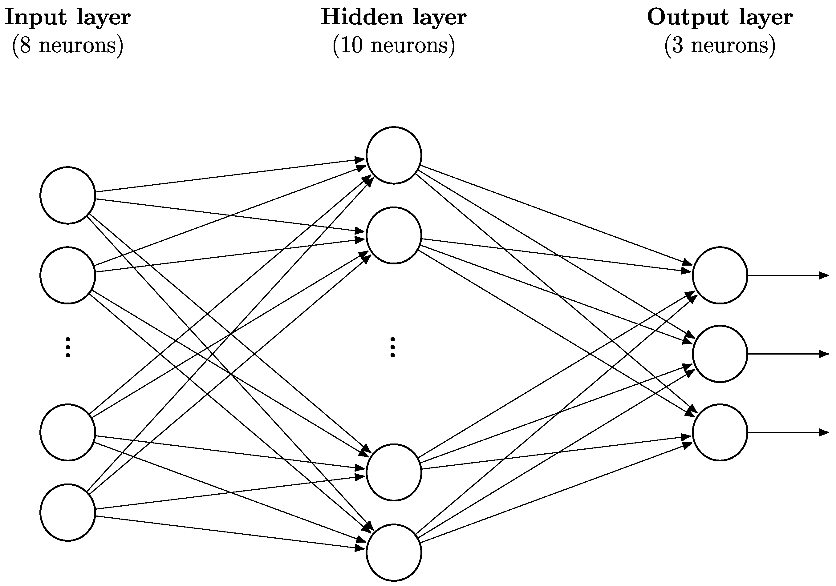
Neural networks are a machine learning technique based loosely on a model of the brain. Inputs are fed into an input layer and then passed to ‘neurons’ in a hidden layer after being multiplied by weights. The neurons in this hidden layer apply an activation function, such as a sigmoid function or a rectified linear unit (ReLU), to the weighted sum of the inputs that they receive. They then pass on this information, again in the form of weights, to neurons either in the next layer, which may be another hidden layer, or the output layer. The central property of a neural network that is useful in machine learning is that a neural network with a single hidden layer of neurons can approximate any continuous function to an arbitrary degree of accuracy, depending on the number of nodes in the hidden layer (
Cybenko 1989).
Figure 1 gives an illustration of the architecture of a neural network with a single hidden layer. Each circle is a node in the network and each line is the weight given to the value being sent from one neuron to a neuron in the next layer. A layer of neurons is known as “dense” or “fully connected” when each neuron in the layer is connected to every neuron in the previous layer. A “feedforward” architecture is one composed of a linear stack of layers where information travels only in one direction through the network, i.e., there are no feedback loops. In this paper, when describing neural networks, an
n1-
n2-
n3 architecture refers to a neural network with
n1 inputs,
n2 nodes in the hidden layer, and
n3 nodes in the output layer. (Note that all neural networks utilized here employ a feedforward architecture with a single, dense hidden layer.) For an introduction to neural networks and their structure, as well as the associated terminology and their use in deep learning problems, see
Nielsen (
2015) or
Bishop (
2006).
Neural network methods and ideas have seen wide use in a variety of applications and have been used to solve problems in the insurance field for at least 25 years. A couple of early applications of neural networks to insurance problems include predicting insolvency or financial distress of insurers (
Park 1993;
Brockett et al. 1994;
Huang et al. 1994) and prediction and regression models related to morbidity or mortality in health and dental insurance (
Tu and Guerriere 1992;
Saemundsson 1996;
Ismael 1999). For a comprehensive account of the early history of neural network use in actuarial science, see
Shapiro (
2002). The use of neural networks in the actuarial area has persisted to present day, with an ever-expanding variety of applications being explored. One very recent example involves using neural networks to more accurately predict claim runoff triangles for various lines of property and casualty insurance (
Kuo 2018). Indeed, researchers have used neural networks to help to speed up calculations related to the pricing and/or hedging of variable annuities with guarantees.
Hejazi and Jackson (
2017) incorporated neural networks in their approach to calculating the solvency capital requirement (SCR) for a large portfolio of VA products; they found that the neural networks yield accurate calculated values while greatly increasing the efficiency of these (otherwise tedious) calculations.
Hejazi and Jackson (
2016) built on the spatial interpolation framework of
Gan and Lin (
2015) using a neural network in place of alternative methods, such as kriging. They found that this neural network approach allows them to estimate the Greeks for a portfolio of VA contracts in a manner that is both accurate as well as more efficient than the alternatives.
In a similar vein, we also used neural networks in the present paper in order to exploit efficiency gains in the tasks of pricing and hedging four types of variable annuity guarantees: GMDB, GMIB, GMAB, and GMWB. Our work differs from the previous research on neural networks mentioned above in two respects. First, we demonstrated a neural network’s performance on predicting liabilities for different market conditions. This demonstrates that a neural network can be used for any Greek calculation, not just deltas, and that once the network is adequately trained, daily MC calculations can be discarded. Second, we explored hedging VA guarantees with a neural network directly, which, to our knowledge, has never been previously explored. For the task of pricing these guarantees, we compared the performance of the neural network to the traditional method of using MC simulations, quantifying the gains in speed, and showing that these gains can be obtained with very little sacrifice in accuracy. With respect to the hedging of the guarantees, we implemented neural network models as an alternative to the traditional delta-rho methodology using MC simulations. We again found that utilizing these neural networks yields significant efficiency gains while very effectively hedging the liability. Further, we explored the impact of the error function used in the training of the neural network on the result for these four types of guarantees. Finally, we note that the neural network hedging methodology presented here is extremely flexible, allowing for different neural network architectures, error functions, and even underlying hedging assets.
The remainder of this article is organized as follows:
Section 2 presents the models and methods (including assumptions made and data used) for the pricing and hedging of the various GMxB products,
Section 3 gives the results of the analysis, comparing the results of the standard pricing and hedging methodologies to those yielded by the neural networks, and
Section 4 concludes with a discussion of the key results and ideas for future work.
2. Methods and Models
In this section, we introduce the assumptions, methods, models, and data used to price and hedge the various VA guarantees. For pricing, we used the traditional method (utilizing MC simulations to estimate the expectations needed for the pricing formulas in
Section 2.2) as a baseline against which to compare the performance of the neural networks. Similarly, for hedging, we used dynamic rebalancing based on calculated delta and rho values as a baseline against which to compare the performance of the neural networks. We also discuss the training of the neural networks used for pricing and hedging.
2.1. Assumptions and Data
We made a number of standard assumptions regarding the various economic, mortality, and policy behavior processes related to the variable annuity products and their associated guarantees. Stock prices are assumed to follow the following stochastic process:
where
St is the stock price at time
t,
σs is the volatility of the stock,
Zs(
t) is a standard Brownian motion process, and
rt is the short rate at time
t, as defined by the Hull-White model (
Hull and White 1990):
where
θ(
t) is determined from a zero-coupon bond yield curve,
a is a mean-reversion parameter for the short rate,
σr is the volatility of the short rate, and
Zr(
t) is a standard Brownian motion process. We assumed that the two standard Brownian motion processes
Zs(
t) and
Zr(
t) are independent.
The size of the wealth account associated with a VA product at time
t is denoted by
Wt and is assumed to follow a similar process to the stock price:
where
δ is the fair fee charged by the insurer for the guarantee. While our assumption was that the wealth account is tied to a single stock index,
Ng and Li (
2013) considered a more complex multiasset framework. We made a static policyholder behavior assumption with no lapses such that 10% of the benefit base for the GMWB is withdrawn at
t = 1, 2, 3, …,
T, and no other withdrawals are made for any other benefit or time. Thus, for
t = 1, 2, 3, …,
T in the case of the GMDB benefit, we have:
where
is set to 10% of the benefit base. Deaths are assumed to follow the Gompertz-Makeham mortality model where the force of mortality for a life age
x is given by:
We fit the parameters of this model using the 1994 VA MGDB ANB life table (
American Academy of Actuaries 2003) and the MortalityLaws package in R (
Pascariu and Canudas-Romo 2018;
R Core Team 2017). The fitted parameters were
α = 0.00025331,
β = 0.07095565, and
λ = 0.00001436. For this study, we assumed that the VA product was issued to a policyholder age 65 and that the term of the contract was
T = 10 years.
For the stock prices, the data we used are the S&P 500 index daily opening prices from 1980 to 1999 (
Yahoo Finance 2018); we estimated the value of
σs using the 5-year rolling historical volatility of this index. For interest rates, we used daily Treasury Yield rate curves from 1990 to 1999 (
U.S. Department of the Treasury 2018). For the parameters in the Hull-White model, we used values of
a = 0.35 and
σr = 0.02, and the value of
θ(
t) was determined from that day’s Treasury yield curve.
2.2. VA Guarantee Pricing Using MC Simulations
Bacinello et al. (
2011) give a thorough overview of pricing each of the common GMxBs in the VA market place. Below is a brief description of the GMxB guarantees and the formulas used to price them. For all results in this paper, 100,000 MC simulations were used to estimate the required expected values; we found that this was adequate to provide stable results.
A GMDB promises the policyholder that if the policyholder dies at some point during the life of the contract, they will receive the maximum of their account value and a guaranteed amount. This guaranteed amount will vary with the specifics of the contract. Typically, the guaranteed amount will be the initial premium, the initial premium accumulated at a specified interest rate, or the maximum account value at any anniversary of the account; we used the latter specification. A GMDB pays off if the policyholder dies during the life of the contract, and the account value is less than the guaranteed amount. If the GMDB is payable at the end of the month of death, the expected present value of the benefits is:
where
is the probability of a policyholder age
x dying in month
k,
N is the number of months until the expiration of the contract, and
G is the largest anniversary value seen to date.
The GMAB insures that the policyholder will receive the greater of their account value and some guarantee amount if they survive to the end of the accumulation phase of the policy. A GMAB pays off if the policyholder is alive and the account value is less than the guaranteed value at the end of the contract so that the expected present value of the benefits is:
where
T is the time until the expiration of the contract and
is the probability of a policyholder age
x surviving
T years.
The GMIB insures that the policyholder will receive a payment stream whose present value is equivalent to the greater of the account value at annuitization, or some minimum guaranteed amount. In the simplest case, the guaranteed amount is an annuitization factor multiplied by the maximum of the initial account value accumulated with interest and the highest anniversary value of the account. If the policyholder chooses a life-contingent annuity, then longevity risk along with financial risk becomes a concern (
Marshall et al. 2010). For simplicity, we followed the assumption made by these authors that all policyholders annuitize uniformly after exactly ten years. A GMIB pays off if the account value is less than the price of an annuity-certain. The annuity-certain used in pricing the GMIB in this study is a 20-year annuity due that pays 5% of the ratcheted guarantee, or the account value, whichever is greater. Thus, the expected present value of the benefits is:
where
a20(
t) is the present value of a 20-year annuity-due that begins payment at time
T.
The GMWB insures that the policyholder will be able to withdraw some fixed amount from their account every year until the benefit amount is depleted, even if the account value is zero. The benefit base is typically set equal to the initial premium and depletes when a withdrawal is made. Pricing a GMWB involves making important assumptions about policyholder behavior.
Milevsky and Salisbury (
2006) and
Bacinello et al. (
2011) both explored the differences between making a static assumption, where the policyholder only withdraws the amount contractually specified, and making a dynamic assumption, where the policyholder makes optimally timed withdrawals.
Luo and Shevchenko (
2015) considered the case of a contract with both GMWB and GMDB benefits, and how their interaction may impact on policyholder behavior. A GMWB pays off if the account value has been depleted, but the policyholder still has the right to make withdrawals. Assuming no lapses and a static withdrawal strategy, where the policyholder is allowed to withdraw up to 10% of the initial investment each year, the expected present value of the benefits is:
where
Bn is the benefit base, ratcheted in proportion to the account value less withdrawals.
Assuming that fees are deducted from the account at the end of each month, the expected present value of the fees is:
and, finally, the liability for a contract on a given day is calculated as the expected present value of the benefits minus the expected present value of the fees.
2.3. Delta-Rho Hedging
A delta-rho hedging methodology was used as a baseline for the neural network’s hedging performance. We assumed that two asset classes were available to be used for the hedge: Shares of the S&P 500 index and a zero-coupon bond with expiration set equal to the expiration of the VA contract, hereafter referred to for simplicity as “stocks” and “bonds”. For each day, the number of stocks and bonds were found such that the combined delta and rho of the portfolio of the GMxB benefit, the stock, and the bond are equal to 0. Finding the deltas and rhos for a benefit on a given day involves two steps. First, four different values are calculated via simulation: The liability if the stock index immediately increased by 1, the liability if the stock index decreased by 1, the liability if the yield curve immediately shifted 1 basis point (bp) up, and the liability if the yield curve shifted 1 bp down. Second, the delta is found by taking the difference between the liabilities where the account value was changed and dividing by two, and the rho is found by taking the difference between the liabilities where the yield curve was changed by one bp and dividing by two. For introductory coverage of Greeks and hedging, see, e.g.,
McDonald (
2012) or
Hull (
2017).
Because of how the Greeks must be calculated, delta-rho hedging increases the amount of time needed to manage a VA portfolio fourfold, because four separate sets of simulations must be run in order to calculate the delta and the rho. For companies with large VA portfolios that can already take a long time to valuate just the liabilities, a fourfold increase in computational time will be expensive, and a hedging solution that does not require as much runtime is preferable.
2.4. Neural Network Pricing Methodology
An alternative to pricing the liability at every day with a Monte Carlo simulation is to train a neural network to predict the liability based only on the same inputs fed to the simulation. (Note that not all of the inputs that are fed to the Monte Carlo simulation are fed to the network, because they are the same for all simulations, i.e., the mortality parameters and Hull-White interest rate model parameters.) Thus, the list of inputs to the pricing neural network is as follows:
Time until maturity of the contract;
Spot rate of the yield curve;
S&P 500 opening price;
Price of a zero-coupon bond maturing at the end of the contract;
Volatility of the S&P 500;
The first three components of a principal component analysis of the yield curve, which are generally interpreted as the height, slope, and curvature of the yield curve;
Fee for the guarantee;
“Moneyness” (M) of the guarantee, defined as M = (G − V)/G, where V is the account value. For the GMWB, G is the amount that the policyholder is allowed to withdraw in a given year. For the other guarantee types, G is the amount guaranteed to the policyholder on their death, survival, or annuitization, respectively. Because this amount ratchets up on policy anniversaries, the guarantee amount represents the highest value seen to date at a policy anniversary.
The sole output of the neural network is the value of the liability for the guarantee. A single hidden layer of ten neurons was used for this neural network, so that the architecture of the network is 10-10-1. Matching the number of neurons in the hidden layer to that in the input layer seems like a reasonable heuristic; this approach has been used to good effect in the past by various researchers (e.g.,
Møller 1993) and produced good results for this study, in the sense that we encountered no problems with overfitting. Nonetheless, when we experimented with other architectures, we found that, in general, increasing the number of nodes in the hidden layer to 15 or 20 only results in marginally better performance, at the expense of longer training times.
2.5. Neural Network Hedging Methodology
An alternative to the classic hedging described above is hedging by training a neural network to buy/sell assets that will minimize the percentage change in the net position of the portfolio of VA liabilities and assets from day to day. This is done by constructing a neural network with the same inputs as the neural network described above to price the guarantees. Like the neural network used for pricing, the network contains a single hidden layer of ten nodes. However, instead of the output layer only containing one node for the liability value, the output layer contains nodes that correspond to different assets used to hedge the portfolio. In this paper, the only assets we assumed available for constructing the hedging portfolio were the same two assets used in the delta-rho hedging methodology, namely “stocks” and “bonds” as described above. Thus, the architecture of the network can be described as 10-10-2. The logic for choosing this architecture parallels that for the pricing neural network, though other configurations could be used. Also, while we only chose to use the two specified assets for this study, we note that one of the benefits of this methodology is its flexibility; it could be made to work with many different sets of available assets.
To summarize the methodology, this hedging neural network uses the same inputs as used in the pricing neural network described above and puts out the quantity of each asset to buy/sell and can be trained to buy/sell assets that will minimize some error function related to the goal of creating the hedge. This reduces the computational cost for obtaining the information needed to hedge the portfolio because a single pass through a neural network involves significantly less computation than simulating a large number of economic paths four different times to find the delta and the rho.
2.6. Neural Network Training
An important aspect of using a neural network for machine learning is training the weights between the nodes in order to better learn the relationship between model inputs and outputs. The simplest algorithm is a so-called “gradient descent”, where the derivative of some error function (typically a sum of squares error function for regression applications, or a cross-entropy error function for classification problems) is taken with respect to each weight. Then, each weight is updated by moving it in the negative direction of its element of the gradient, scaled by some learning rate. A challenge associated with this approach is that if the learning rate is too large, the network will skip over global or local minima and never converge, and if the learning rate is too small, training will take a long time to converge. For this study, the error function chosen was a key determinant in the performance of the neural network; in
Section 3.2, we explore the ramifications of changing the error function.
Alternatives to gradient descent include the resilient backpropagation algorithm (RPROP), scaled conjugate gradient descent (SCGD), and the Broyden-Fletcher-Goldsharb-Shanno algorithm (BFGS). (
Riedmiller 1994;
Møller 1993) RPROP is an algorithm that updates each weight only based on the sign of the gradient. It then increases the size of the step for each weight as long as that weight maintains the sign for its gradient. If the sign of the gradient for a particular weight changes, the size of the step for that weight is decreased and the step size begins moving in the opposite direction. RPROP is fast, initially, because it uses only first order information but can be slower to converge overall because the use of only first order information makes it difficult for the algorithm to converge towards the end of training.
SCGD is an algorithm that improves on simple gradient descent using a second order approximation to the error function to find an appropriate learning rate at each iteration. BFGS uses a more complete second order approximation and also a line search to determine the appropriate step size and direction for each weight.
For the results in this paper, the BFGS algorithm was used as implemented in the nnet package in R (
Venables and Ripley 2002;
R Core Team 2017). However, parts of the analysis were also run with the SCGD algorithm, with comparable performance. We found that the RPROP algorithm provides a faster initial reduction in error but converges to a desired level of accuracy more slowly than with the other two algorithms, and sometimes fails to converge entirely.
We prepared the dataset by splitting the data into a training set and a testing set. Specifically, 80% of the data were used for the training set, while the remaining 20% were used for testing; we randomly chose the points to be placed into each set. There were in total 2530 data points, 2023 of which were used for training, while the remaining 507 were used for testing. This method of partitioning the data for training and testing (i.e., a randomly chosen 80/20 split) is rather common in neural network applications.
4. Conclusions
The results of the previous section demonstrate that neural networks can indeed be used effectively to price as well as hedge various types of VA GMxB guarantees. When using neural networks in this manner, we see a significant gain in efficiency (speed) when compared to the traditional pricing and hedging methodologies. In some cases, the performance of the neural network was markedly superior, whereas in other cases, the performance is comparable to traditional methods, but in all cases, the relative efficiency gains were quite significant.
In some hedging scenarios, the neural network can tend to overinvest to assets to form the hedge portfolio, sometimes resulting in unreasonably large capital requirements. Using different tolerance thresholds in the error function when training the network can largely control this tendency and can significantly impact on the results; there is often a tradeoff between quality of the hedge (as measured by our HE1 metric) and the cost of capital required for the hedging assets. Of course, whether this tradeoff is worthwhile will depend on the cost of capital relative to the benefit of the more efficient calculations, cost of computing resources, and other considerations.
In this paper, we have demonstrated that there can be significant efficiency gains over traditional models when we utilize neural networks for the pricing of various VA guarantees; we found these gains consistently over four of the more popular types of GMxB guarantees: GMDB, GMAB, GMDB, and GMWB. We have also shown that it is possible to use neural networks to hedge these types of VA guarantees, as an alternative to the traditional delta-rho methodology using MC simulations. We have experimented with different tolerances (thresholds) in the error function used to train the neural networks and have examined the resulting hedging performance using a variant of the HE1 metric. In all cases, the neural networks exhibited promising results.
There are several possible avenues for future work in this line of research. We have shown that the error function can have a significant effect on the performance of a neural network; while we have experimented with various thresholds, it may also be worthwhile to consider different forms of error functions and to measure the resulting performance, especially given the large impact that the error function and threshold has been shown to make in terms of both hedging performance and speed. In addition, while the HE1 hedging metric we used here seems to be a reasonable method for capturing the performance of the hedge for these guarantees, many other metrics are possible and have been used by various researchers. It would be instructive to repeat this type of study using some of the other measures. In addition, it may be helpful to generalize the results obtained here by applying this methodology to other time periods. The time period used here was chosen arbitrarily in order to demonstrate the methodology, but a deeper look into the relative performance of the neural network over different times periods spanning a broad range of interest rate and stock market conditions would seem to be warranted. Further, while our model accounts for mortality, it does not incorporate elements of policyholder behavior, such as lapses or dynamic withdrawal behavior. As neural networks are very flexible, they could certainly be trained to incorporate these important aspects of variable annuities. Finally, one of the most significant benefits of using the neural network to hedge is the flexibility of choice of hedging assets. While we used only two assets here, namely a stock index and bond, the neural network approach could be used with virtually any number and/or type of assets. There is an opportunity to explore this idea and determine which combinations of asset types are most effective for hedging the various types of VA guarantees.


